LATEX maths and graphics - Department of Engineering

L ATEX maths and graphics
Tim Love
July 27, 2006
This handout assumes that you have already read the Advanced LaTeX 1 document.
Note that there’s an alternative way of producing maths in L ATEX - AMS-L ATEX. See the online manual
2 for details.
If you want to more more about graphics, see Using Imported Graphics in LaTeX and PDFLaTeX 3
by Keith Reckdahl.
Comments and bug reports to Tim Love (tpl@eng.cam.ac.uk).
Contents
1 Maths 2
1.1 Environments . . . . . . . . . . . . . . . . . . . . . . . . . . . . . . . . . . . . . . . . . . . . . . . . . . 2
1.2 Special Characters . . . . . . . . . . . . . . . . . . . . . . . . . . . . . . . . . . . . . . . . . . . . . . . . 3
1.2.1 Greek . . . . . . . . . . . . . . . . . . . . . . . . . . . . . . . . . . . . . . . . . . . . . . . . . . . 3
1.2.2 Miscellaneous . . . . . . . . . . . . . . . . . . . . . . . . . . . . . . . . . . . . . . . . . . . . . . 3
1.2.3 Arrows . . . . . . . . . . . . . . . . . . . . . . . . . . . . . . . . . . . . . . . . . . . . . . . . . . 4
1.2.4 Calligraphic . . . . . . . . . . . . . . . . . . . . . . . . . . . . . . . . . . . . . . . . . . . . . . . 4
1.2.5 Character Modifiers . . . . . . . . . . . . . . . . . . . . . . . . . . . . . . . . . . . . . . . . . . 4
1.2.6 Common functions . . . . . . . . . . . . . . . . . . . . . . . . . . . . . . . . . . . . . . . . . . . 5
1.3 Subscripts and superscripts . . . . . . . . . . . . . . . . . . . . . . . . . . . . . . . . . . . . . . . . . . 5
1.4 Overlining, underlining and bold characters . . . . . . . . . . . . . . . . . . . . . . . . . . . . . . . . 6
1.5 Roots and Fractions . . . . . . . . . . . . . . . . . . . . . . . . . . . . . . . . . . . . . . . . . . . . . . . 6
1.6 Delimiters . . . . . . . . . . . . . . . . . . . . . . . . . . . . . . . . . . . . . . . . . . . . . . . . . . . . 6
1.7 Numbering and labelling . . . . . . . . . . . . . . . . . . . . . . . . . . . . . . . . . . . . . . . . . . . 7
1.8 Matrices . . . . . . . . . . . . . . . . . . . . . . . . . . . . . . . . . . . . . . . . . . . . . . . . . . . . . 8
1.9 Macros . . . . . . . . . . . . . . . . . . . . . . . . . . . . . . . . . . . . . . . . . . . . . . . . . . . . . . 9
1.10 Packages . . . . . . . . . . . . . . . . . . . . . . . . . . . . . . . . . . . . . . . . . . . . . . . . . . . . . 9
1.11 Fine tuning . . . . . . . . . . . . . . . . . . . . . . . . . . . . . . . . . . . . . . . . . . . . . . . . . . . . 9
1.12 Maths and Postscript fonts . . . . . . . . . . . . . . . . . . . . . . . . . . . . . . . . . . . . . . . . . . . 10
1.13 Matlab and LaTeX . . . . . . . . . . . . . . . . . . . . . . . . . . . . . . . . . . . . . . . . . . . . . . . . 10
1.14 Examples . . . . . . . . . . . . . . . . . . . . . . . . . . . . . . . . . . . . . . . . . . . . . . . . . . . . . 11
1 http://www-h.eng.cam.ac.uk/help/tpl/textprocessing/latex advanced/latex advanced.html
2 http://www-h.eng.cam.ac.uk/help/tpl/textprocessing/amslatex.dvi
3 http://www-h.eng.cam.ac.uk/help/tpl/textprocessing/epslatex.ps
Copyright c○2004-6 by T.P. Love. This document may be copied freely for the purposes of education and noncommercial
research. Cambridge University Engineering Department, Cambridge CB2 1PZ, England.
1

2 Graphics 12
2.1 Postscript . . . . . . . . . . . . . . . . . . . . . . . . . . . . . . . . . . . . . . . . . . . . . . . . . . . . . 12
2.1.1 psfrag: adding maths to postscript files . . . . . . . . . . . . . . . . . . . . . . . . . . . . . . 13
2.1.2 Postscript from PCs/Macs . . . . . . . . . . . . . . . . . . . . . . . . . . . . . . . . . . . . . . . 13
2.2 Scaling, rotation, clipping, wrap-around and shadows . . . . . . . . . . . . . . . . . . . . . . . . . . . 14
2.3 GIF and jpeg files . . . . . . . . . . . . . . . . . . . . . . . . . . . . . . . . . . . . . . . . . . . . . . . . 15
2.4 PStricks . . . . . . . . . . . . . . . . . . . . . . . . . . . . . . . . . . . . . . . . . . . . . . . . . . . . . . 16
1 Maths
There’s more to maths typesetting than meets the eye. Many conventions used in the typesetting of plain text are
inappropriate to maths. L ATEX goes a long way to help you along with the style. For example, in a L ATEX maths
environment, letters come out in italics, ‘-’ as ‘−’ (minus) instead of the usual ‘-’ (dash), ‘*’ becomes ∗, ’ becomes
′ and spacing is changed (less around ‘/’, more around ‘+’).
Many of the usual L ATEX constructions can still be used in maths environments but their effect may be slightly
different; eg \textbf{ } only affects letters and numbers. ‘{’ and ‘}’ are still special characters; they’re used to
group characters.
As usual in L ATEX you can override the defaults, but think before doing it: maths support in L ATEX has been
carefully thought out and is quite logical though the L ATEX source text may not be very readable. It’s a good
idea to write out the formulae on paper before you start L ATEXing, and try not to overdo the use of the ‘\frac’
construction; use ‘/’ instead.
1.1 Environments
There are 2 environments to display one-line equations.
equation:- Equations in this environment are numbered.
\begin{equation}
x + iy
\end{equation}
x + iy (1)
displaymath:- These won’t be numbered. \[, \] can be used as abbreviations for \begin{displaymath} and
\end{displaymath}.
\begin{displaymath}
x + iy
\end{displaymath}
x + iy
Never leave a blank line before these equations; it starts a new paragraph and looks ugly. ’\displaystyle’ is
the font type used to print maths in these display environments. Other relevant environments are:-
math:- For use in text. \( and \) can be used to delimit the environment, as can the TEX constructions $ and $ .
For example, $x=yˆ2$ gives x = y 2 .
eqnarray:- This is like a 3 column tabular environment. Each line by default is numbered. You can use the
eqnarray* variant to suppress numbering altogether.
2

\begin{eqnarray}
a1 & = & b1 + c1\nonumber\\
a2 & = & b2 - c2
\end{eqnarray}
a1 = b1 + c1
a2 = b2 − c2 (2)
Maths in “display” and “inline” environments have different default sizes for some characters and other behavioural
differences so that a line of maths won’t impinge on text lines below or above. If you want to put some
non-maths text in amongst maths then enclose it in an \mbox{...}.
1.2 Special Characters
The The Comprehensive LaTeX Symbol List 4 document offers 105 pages of symbols. Here are just a few.
1.2.1 Greek
1.2.2 Miscellaneous
α \alpha β \beta γ \gamma δ \delta ɛ \epsilon
ζ \zeta η \eta θ \theta ι \iota κ \kappa
λ \lambda µ \mu ν \nu ξ \xi o o
π \pi ρ \rho σ \sigma τ \tau υ \upsilon
φ \phi χ \chi ψ \psi ω \omega Γ \Gamma
∆ \Delta Θ \Theta Λ \Lambda Ξ \Xi Π \Pi
Σ \Sigma Υ \Upsilon Φ \Phi Ψ \Psi Ω \Omega
. . . \ldots · · · \cdots
. \vdots
. .. \ddots ± \pm ∓ \mp
× \times ÷ \div ∗ \ast
⋆
·
∪
�
�
∧
\star
\cdot
\cup
\biguplus
\bigsqcup
\wedge
◦
∩
�
⊓
∨
�
\circ
\cap
\bigcup
\sqcap
\vee
\bigwedge
•
�
⊎
⊔
�
\
\bullet
\bigcap
\uplus
\sqcup
\bigvee
\setminus
≀ \wr ⋄ \diamond △ \bigtriangleup
▽
⊕
⊗
⊙
\bigtriangledown
\oplus
\otimes
\odot
⊳
�
�
�
\triangleleft
\bigoplus
\bigotimes
\bigodot
⊲
⊖
⊘
○
\triangleright
\ominus
\oslash
\bigcirc
∐ \amalg ≤ \leq ≺ \prec
� \preceq ≪ \ll ⊂ \subset
⊆ \subseteq ⊑ \sqsubseteq ∈ \in
⊢ \vdash ≥ \geq ≻ \succ
4 http://www.tex.ac.uk/tex-archive/info/symbols/comprehensive/symbols-a4.pdf
3

1.2.3 Arrows
� \succeq ≫ \gg ⊃ \supset
⊇ \supseteq ⊒ \sqsupseteq ∋ \ni
⊣ \dashv ≡ \equiv ∼ \sim
�
∼=
\simeq
\cong
≍
�=
\asymp
\neq
≈
.
=
\approx
\doteq
∝ \propto |= \models ⊥ \perp
| \mid � \parallel ⊲⊳ \bowtie
⌣ \smile ⌢ \frown ℵ \aleph
� \hbar ı \imath j \jmath
ℓ \ell ℘ \wp ℜ \Re
ℑ
∇
\Im
\nabla
′
√
\prime
\surd ⊤
\empty
\top
⊥ \bot � \| ∠ \angle
∀ \forall ∃ \exists ¬ \neg
♭ \flat ♮ \natural ♯ \sharp
\
�
△
\backslash
\triangle
\coprod
∂
�
�
\partial
\sum
\int
∞
�
�
\infty
\prod
\oint
← \leftarrow ⇐ \Leftarrow → \rightarrow
⇒ \Rightarrow ↔ \leftrightarrow ⇔ \Leftrightarrow
↦→ \mapsto ←↪ \hookleftarrow ↼ \leftharpoonup
↽ \leftharpoondown ⇋ \rightleftharpoons ←− \longleftarrow
⇐= \Longleftarrow −→ \longrightarrow =⇒ \Longrightarrow
←→ \longleftrightarrow ⇐⇒ \Longleftrightarrow ↦−→ \longmapsto
↩→ \hookrightarrow ⇀ \rightharpoonup ⇁ \rightharpoondown
↑ \uparrow ⇑ \Uparrow ↓ \downarrow
⇓ \Downarrow ↕ \updownarrow ↗ \nearrow
↘ \searrow ↙ \swarrow ↖ \nwarrow
1.2.4 Calligraphic
These characters are available if you use the \mathcal control sequence.
${\mathcal A B C D E F G H I J K L M N O P Q R S T U V W X Y Z}$
gives ABCDEF GHIJKLMNOP QRST UV W XY Z
Also useful are “blackboard” style characters. \mathbb{ R Q Z} gives RQZ (requires the amsfonts package).
1.2.5 Character Modifiers
�
\hat{e} ê \widehat{easy} easy �
\tilde{e} ˜e \widetilde{easy} easy �
\check{e} ě \breve{e} ĕ
\acute{e} é \grave{e} è
\bar{e} ē \vec{e} �e
\dot{e} ˙e \ddot{e} ë
\not e e
4

Note that the wide versions of hat and tilde cannot produce very wide alternatives. The ‘\not’ operator hasn’t
properly cut the following letter. The Fine Tuning section on page 9 describes how to adjust this.
If you want to place one character above another, you can use \stackrel, which prints its first argument in
small type immediately above the second
$ a \stackrel{def}{=} b + c $
gives a def
= b + c
See the Macros section for how to stack characters using atop.
1.2.6 Common functions
In a maths environment, L ATEX assumes that variables will have single-character names. Function names require
special treatment. The advantage of using the following control sequences for common functions is that the text
will not be put in math italic and subscripts/superscripts will be made into limits where appropriate.
\arccos \arcsin \arctan \arg \cos \cosh \cot
\coth \csc \deg \det \dim \exp \gcd
\hom \inf \ker \lg \lim \liminf \ln
\log \max \min \Pr sec \sin \sinh
\sup \tan \tanh
1.3 Subscripts and superscripts
These are introduced by the ‘ˆ’ and ‘_’ characters. Depending on the base character and the current style, the subor
superscripts may go to the right of or directly above/below the main character. With letters it goes to the right.
$F_2ˆ3$
produces ‘F 3 2 ’. Note that the sub- and superscripts aren’t in line. To make them so, you can add an invisible
character after the ‘F’. $F{}_2ˆ3$ produces F 3 2 .
With � the default behaviour is different in display and text styles.
$\sum_{i=0}ˆ2 $
produces �2 i=0 (text style) but
\[\sum_{i=0}ˆ2 \]
produces (in display style)
This default behaviour can be overridden, if you really need to. For example in text mode,
$\sum\limits_{i=0}ˆ2$
produces 2�
i=0
2�
i=0
5

1.4 Overlining, underlining and bold characters
$\underline{one} \overline{two}$
produces onetwo. This is not a useful facility if it’s used more than once on a line. The lines are produced so that
they don’t quite overlap the text; lines over or under different words won’t in general be at the same height.
To be able to reproduce bold maths, it’s best to use the bm package. $E = \bm{mcˆ2}$ produces E = mc2 .
Alternatively, you can use \mathbf{} to create bold characters - $\mathbf{F}_2ˆ3$ produces F3 2 . or you
can use the following idea
\usepackage{amsbsy} % This loads amstext too
\begin{document}
$\omega + \boldsymbol{\omega}$
% Use the following if whole expressions need to be in bold
{\boldmath $\omega $}
\end{document}
1.5 Roots and Fractions
$\sqrt{4} + \sqrt[3]{x + y}$
gives √ 4 + 3√ x + y.
Three constructions for putting expressions above others are
frac:- $\frac{1}{(x + 3)}$ produces 1
(x+3) .
choose:- ${n + 1 \choose 3}$ produces � � n+1
3 .
atop:- ${x \atop y}$ produces x
y .
These constructions can be used with ones described earlier. E.g.,
\[ \sum_{-1\le i \le 1 \atop 0 < j < \infty} f(i,j)\]
gives
1.6 Delimiters
�
−1≤i≤1
0

This table shows the standard sizes. To get bigger sizes, use these prefices
(for left delimiters) (for right delimiters) magnification
\bigl \bigr a bit bigger, but won’t overlap lines
\Bigl \Bigr 150% times big
\biggl \biggr 200% times big
\Biggl \Biggr 250% times big
For example,
$\Biggl\{2\Bigl(x(3+y)\Bigr)\Biggr\}$
�
� �
gives 2 x(3 + y)
�
. If you’re not using the default text size these commands might not work correctly. In that
case try the exscale package.
It’s preferable to let L ATEX choose the delimiter size for you by using \left and \right. These will produce
delimiters just big enough for the formulae inbetween.
$\left( \frac{(x+iy)}{\{\int x\}} \right)$
�
gives
� (x+iy)
{ R x}
The left and right delimiters needn’t be the same type. It’s sometimes useful to make one of them invisible
\[ z = \left\{
\begin{array}{ll}
1 & (x>0)\\
0 & (x 0)
0 (x < 0)
$\overbrace{\alpha \ldots \omega}ˆ{\mbox{greek}}
\underbrace{a \ldots z}_{\mbox{english}}$
greek
� �� �
produces α . . . ω a
�
.
��
. . z
�
. The use of \mbox stops the text appearing in math italic.
english
1.7 Numbering and labelling
Numbering happening automatically when you display equations. If you don’t want an equation numbered, use
\nonumber beside the equation. Equation numbers appear to the right of the maths by default. To make them
appear on the left use the leqno class option (i.e., use \documentclass[leqno,....]{....}).
Use \label{} to label an equation (or figure, section etc) in order to reference from elsewhere.
\begin{equation}
W_{\bf S}(t,\omega) = \int\limits_{-\infty}ˆ{\infty} {
{\cal R}_{\bf S}(t,\tau) eˆ{-j\omega\tau} \,d \tau }
\label{LABELLING}
\end{equation}
7

Now the following text
WS(t, ω) =
refers back to equation \ref{LABELLING}
refers back to equation 3 by number, and
refers back to the equation on page \pageref{LABELLING}
�∞
−∞
RS(t, τ)e −jωτ dτ (3)
refers back to the equation on page 8.
A file will have to be L ATEX’ed twice before the references, both forwards and backwards, will be correctly
produced.
1.8 Matrices
The array environment is like L ATEX’s tabular environment except that each element is in math mode. The
number and alignment of columns is controlled by the arguments - use l, c or r to represent each column with
either left, center or right alignment. The default font style used is \textstyle but you can override this by
changing the \displaystyle.
\begin{math}
\begin{array}{clrr} %
a+b+c & uv & x-y & 27 \\
x+y & w & +z & 363
\end{array}
\end{math}
a + b + c uv x − y 27
produces
x + y w +z 363
The rows are arranged so that their centres are aligned. You can align their tops or bottoms instead by using a
further argument when you create the array.
\begin{array}{clrr}[t]
would produce top-aligned lines, and ‘[b]’ would produce bottom-aligned ones. The Delimiters section of this
document shows how to bracket matrices.
TEX has a few maths facilities not mentioned in the L ATEX book. The following TEX construction might be useful.
\begin{math}
\bordermatrix{&a_1&a_2&...&a_n\cr
b_1 & 1.2 & 3.3 & 5.1 & 2.8 \cr
c_1 & 4.7 & 7.8 & 2.4 & 1.9 \cr
... & ... & ... & ... & ... \cr
z_1 & 8.0 & 9.9 & 0.9 & 9.99 \cr}
\end{math}
a1 a2 ... an
⎛
b1 1.2
c1 ⎜ 4.7
... ⎝ ...
3.3
7.8
...
5.1
2.4
...
⎞
2.8
1.9 ⎟
... ⎠
z1 8.0 9.9 0.9 9.99
8

1.9 Macros
These aid readability, save on repetitive typing and offer ways of producing stylistic variations on standard L ATEX
formats.
\def\bydefn{\stackrel{def}{=}}
\def\convf{\hbox{\space \raise-2mm\hbox{$\textstyle
\bigotimes \atop \scriptstyle \omega$} \space}}
produce def
= and �
1.10 Packages
ω
when $\bydefn$ and $\convf$ are typed.
The following packages may be of help - easybmat 5 (easy block matrices), easyeqn 6 (easy equations), easymat 7
(easy matrices), easytable 8 (easy tables), easyvector 9 (easy vectors), delarray 10 (nested arrays), theorem 11 (gives
more choice in theorem layout), subeqnarray (Renumbering of sub-arrays in math-mode), subeqn (Different
numbering sub-arrays).
1.11 Fine tuning
It’s generally a good idea to keep punctuation outside math mode; L ATEX’s normal handling of spacing around
punctuation is suspended during maths. Sometimes you might want to adjust the spacing in a formula (e.g., you
might want to add space before dx). Use these symbols :a\,
b (a b) thin space
a\> b (a b) medium space
a\; b (a b) thick space
a\! b (ab) negative thin space
Long math expressions aren’t broken automatically unless you use the breqn 12 package, which is still a little
experimental. In an eqnarray environment you may want to break a long line manually. You can do this by
putting
y & = & a + b \nonumber \\
& & + k
to give
y = a + b
+k (4)
but the spacing around the ‘+’ on the 2nd line is wrong because L ATEX thinks it’s a unary operator. You can fool
L ATEX into treating it as a binary operator by inserting a hidden character.
y & = & a + b \nonumber \\
& & \mbox{} + k
5 http://www-h.eng.cam.ac.uk/help/tpl/textprocessing/easybmat.dvi
6 http://www-h.eng.cam.ac.uk/help/tpl/textprocessing/easyeqn.dvi
7 http://www-h.eng.cam.ac.uk/help/tpl/textprocessing/easymat.dvi
8 http://www-h.eng.cam.ac.uk/help/tpl/textprocessing/easytable.dvi
9 http://www-h.eng.cam.ac.uk/help/tpl/textprocessing/easyvector.dvi
10 http://www-h.eng.cam.ac.uk/help/tpl/textprocessing/delarray.dvi
11 http://www-h.eng.cam.ac.uk/help/tpl/textprocessing/theorem.dvi
12 http://www-h.eng.cam.ac.uk/help/tpl/textprocessing/breqndoc.dvi
9

gives
y = a + b
+ k (5)
You can use the \lefteqn construction to format long expressions so that continuation lines are differently
indented.
\begin{eqnarray}
\lefteqn{x+ iy=}\\
& & a + b + c + d + e + f + g + h + i + j + k +\nonumber\\
& & l + m \nonumber
\end{eqnarray}
x + iy = (6)
a + b + c + d + e + f + g + h + i + j + k +
l + m
If you want more vertical spacing around a line you can create an invisible vertical ”struct” in LaTeX. creates
a box of width 0, height 1cm which starts .3cm below the usual line base, use \rule[-.3cm]{0cm}{1cm}. By
adjusting these values you should be able to create as much extra space below/above the maths as you like. “ A
B
and” is created by
$A \over B$ \rule[-.3cm]{0cm}{1cm}{and}
1.12 Maths and Postscript fonts
It’s easy to use a postscript font (like helvetica) for the text of a L ATEX document. What’s harder is using the same
font for maths - the font will lack many of the special characters required for maths. An easy, reasonable option is
to use the mathptmx package to put the maths into the postscript Times and symbol fonts where possible.
Alternatively, use
• the mathpazo package (loads Palatino as the text font family and a mixture of the Pazo and CM fonts for
math).
• the mathpple package (loads Palatino as the text font family and a mixture of artificially obliqued Euler
fonts and CM fonts for math).
Commercial and free alternatives are under development. See Stephen G. Hartke’s A Survey of Free Math
Fonts for TeX and LaTeX 13 for details.
1.13 Matlab and LaTeX
Matlab 14 has some support for LaTeX production. For example
latex(’(sin(x)+2*x+3*xˆ2)/(5*x+6*xˆ2)’,’math.tex’)
puts the LaTeX representation of the expression into a file called math.tex. Type “help latex" inside matlab
for details.
13 http://ctan.tug.org/tex-archive/info/Free Math Font Survey/survey.html
14 http://www-h.eng.cam.ac.uk/help/tpl/programs/matlab.html
10

1.14 Examples
• \begin{eqnarray}
{\cal M}ˆ2(\hat{\theta},\theta) &=& E[(\hat{\theta} - \theta)ˆ2]
\nonumber \\
{\cal M}ˆ2(\hat{\theta},\theta) &=& {\rm var}ˆ2(\hat{\theta}) +
{\cal B}ˆ2(\hat{\theta}).
\end{eqnarray}
gives
M 2 ( ˆ θ, θ) = E[( ˆ θ − θ) 2 ]
• \begin{equation}
\hat{W}_{s}(t,\omega;\phi) \bydefn
\int\limits_{-\infty}ˆ{\infty}
{\hat{\cal R}_s(t,\tau;\psi) eˆ{-j\omega \tau}
\, d \tau }
\end{equation}
gives
M 2 ( ˆ θ, θ) = var 2 ( ˆ θ) + B 2 ( ˆ θ). (7)
ˆWs(t, ω; φ) def
=
�∞
−∞
• \begin{eqnarray}
{\cal B}(t,\omega) & \approx &
{1 \over 4\pi}
{\cal D}_tˆ2 W_{\bf S}(t, \omega)
{{{\scriptstyle \infty} \atop
{\displaystyle \int \! \int \!
}}\atop {\scriptstyle -\infty}}
t_1ˆ2
\phi(t_1,\omega_1) \, dt_1 d\omega_1
\nonumber \\
&& +
{1 \over 4\pi}
{\cal D}_\omegaˆ2 W_{\bf S}(t, \omega)
{{{\scriptstyle \infty} \atop
{\displaystyle \int \! \int \!
}}\atop {\scriptstyle -\infty}}
\omega_1ˆ2
\phi(t_1,\omega_1) \, dt_1 \, d\omega_1.
\label{F4}
\end{eqnarray}
gives
B(t, ω) ≈ 1
4π D2 t WS(t,
�∞� ω)
+ 1
4π D2 ω WS(t, ω)
11
ˆRs(t, τ; ψ)e −jωτ dτ (8)
−∞
∞
� �
−∞
t 2 1 φ(t1, ω1) dt1dω1
ω 2 1 φ(t1, ω1) dt1 dω1. (9)

• \newsavebox{\DERIVBOXZLM}
\savebox{\DERIVBOXZLM}[2.5em]{$\Longrightarrow\hspace{-1.5em}
\raisebox{.2ex}{*}
\hspace{-.7em}\raisebox{-.8ex}{\scriptsize lm}\hspace{.7em}$}
\newcommand{\Deriveszlm}{\usebox{\DERIVBOXZLM}}
\Deriveszlm
gives
=⇒ *
lm
2 Graphics
Graphics can be produced
• from within LaTeX - pictures can be drawn in a picture environment, but you’ll find graph paper handy
(xfig can create code for the picture environment). The pstricks packages (see page 16) is far more
powerful.
• by any program that can produce Postscript files (for LaTeX) or JPEG, PNG andPDF (for pdflatex).
Whatever graphics you want to add, you should use the figure environment so that L ATEX can cope sensibly
with situations where, for example, you attempt to insert near the bottom of a page a graphic that’s half a page
high. The figure environment will float the graphic to the top or bottom of the page, or on the next page, with
preferences that you can provide.
h here
t top of page
b bottom of page
p on a page with no text
Putting ! as the first argument in the square brackets will encourage L ATEX to do what you say, even if the
result’s sub-optimal. See the online hints about floats in LaTeX 15 for further details.
\begin{figure}[htbp]
\vspace{0.5in}
\caption{0.5 inch of space}
\end{figure}
Figure 1: 0.5 inch of space
It’s possible to have more than one graphic in a figure. See the example later on.
2.1 Postscript
pdflatex supports JPEG, PNG andPDF images - but not postscript. latex supports Postscript files as long as
they have a proper bounding box comment; i.e. L ATEX requires full Encapsulated Postscript 16 as produced by (for
15 http://www-h.eng.cam.ac.uk/help/tpl/textprocessing/float hint.html
16 http://www-h.eng.cam.ac.uk/help/tpl/graphics/postscript.html
12

example) Xfig 17 on Unix. If the file hasn’t got a BoundingBox line near the top, you can use ps2epsi to generate
one. Wherever the postscript file comes from, simply use
\documentclass[dvips]{article}
\usepackage{graphicx}
then include the postscript file using the following commands
\begin{figure}[htbp]
\includegraphics{yourfile.ps}
\end{figure}
L ATEX can cope with compressed postscript files too, but since latex can’t read the BoundingBox line from the
compressed file, you need to provide it. If your compressed file’s called yourfile.ps.gz, copy the BoundingBox
line into a file called yourfile.ps.bb. Then the following works
\begin{figure}[htbp]
\includegraphics{yourfile.ps.gz}
\end{figure}
Just about all of the following facilities use postscript. You’ll need to run latex to generate ‘foo.dvi’, then
run dvips -o foo.ps foo.dvi to convert the resulting DVI/postscript file to pure postscript. This will produce
a file that can be previewed with ghostview or gs.
2.1.1 psfrag: adding maths to postscript files
Many packages that produce postscript output don’t provide good maths facilities. It’s often easier to add the
maths in later using the psfrag package. This lets you replace text in a postscript file (produced with xfig,
matlab, etc) by a fragment of L ATEX. For example, doing
\usepackage{psfrag}
...
\begin{figure}
\psfrag{MATHS}{$xˆ2$}
\includegraphics{foo.eps}
\end{figure}
would display the file with MATHS replaced by x 2 . See the online documentation 18 for details.
2.1.2 Postscript from PCs/Macs
Modern applications should generate a conforming EPS file. Under windows when you’re printing to file, look at
the PostScript properties (or Advanced options), and choose (depending on the driver you have) either ’Archive
Format’, ’Encapsulated PS’, ’Optimize for Portability’ or ’Page Independence’. People seem to have more luck
with the free Adobe postscript driver than with the Microsoft one.
The resulting file should begin with %!. If it doesn’t it’s not postscript. Remove any characters that are before
%!PS, and (to be on the safe side) remove anything after the final %%EOF line.Platform-specific considerations do
crop up. The EPS generated on Macintoshes will use ASCII 13 line terminators, while Unix will use ASCII 10
(and DOS will use both). If this causes trouble, use emacs to convert, or try (in Unix)
tr "\015" "\012" new.ps
17 http://www-h.eng.cam.ac.uk/help/tpl/graphics/xfig/xfig.html
18 http://www-h.eng.cam.ac.uk/help/tpl/textprocessing/psfrag.ps
13

2.2 Scaling, rotation, clipping, wrap-around and shadows
The graphicx package includes routines that are useful even without graphics. \reflectbox{Reflect} pro-
and \resizebox{3cm}{0.2cm}{Stretched} produces Stretched. To scale imported
graphics, use some optional arguments
ducesReflect
\includegraphics[width=5cm,height=10cm]{yourfile.ps}
would rescale the postscript so that it was 5cm wide and 10cm high. To make the picture 5cm wide and scale the
height in proportion use
\includegraphics[width=5cm]{yourfile.ps}
To rotate anticlockwise by the specified number of degrees, use
\includegraphics[angle=150]{yourfile.ps}
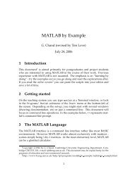
These options can be combined - note that order matters. The following examples demonstrate how to combine
these features and how to use the subfig package to have more than one graphic in a figure.
Figure 2: Tigers
\centering
\begin{figure}[hbtp]
\includegraphics[height=40mm]{/export/ghostfonts/tiger.eps}
\includegraphics[angle=120, height=20mm]{/export/ghostfonts/tiger.eps}
\caption{Tigers}
\end{figure}
% remember to do \usepackage{subfig} at the top of the document!
\begin{figure}[hbtp]
\centering
\subfloat[Small]% \quad on the next line adds spacing
{\includegraphics[height=30mm]{/export/ghostfonts/crest.eps}}\quad
\subfloat[Medium]
{\includegraphics[width=40mm]{CUni3.eps}}\quad
\subfloat[Large]
{\includegraphics[height=50mm]{/export/ghostfonts/crest.eps}}
\caption{3 crests}
\end{figure}
14

(a) Small (b) Medium (c) Large
Figure 3: 3 crests
To clip the postscript image use the viewpoint argument. The following fragment would display only part
of the image. The viewport coordinates are in the same units as the bounding box.
\begin{figure}[htbp]
\includegraphics[viewport=200 400 400 600,width=5cm,clip]%
{CUniv3.eps}
\end{figure}
% Use the floatflt package
\begin{floatingfigure}[l]{4cm}
\includegraphics[width=2cm]{/export/ghostfonts/crest.eps}
\caption{Using floatingfigure}
\end{floatingfigure}
Figure 4: Using floatingfigure
The floatflt19 package lets you insert a graphic and have the text wrap around
it. You can provide 2 arguments to the floatingfigure command: the first (l or
r) selects whether you want the graphic to be on the left or right of the page. The 2nd
argument gives the width of the graphic. Not all text will flow perfectly around (for
example, verbatim text fails, as illustrated below) so check the final output carefully.
Using the fancybox package gives you access to \shadowbox, \ovalbox, \Ovalbox
and \doublebox commands, which can be used with text or with graphics. For ex-
shadow package
ample, \shadowbox{shadow package} produces
and
\ovalbox{\includegraphics[height=10mm]{CUni3.eps}}
✎
2.3 GIF and jpeg files
☞
produces ✍
✌ . Unfortunately, the fancybox package as
supplied suppresses the table of contents. The locally produced contentsfancybox
solves this, but may introduce graphics problems.
CUED users can include a file called keyboard.gif, for example, by doing gif2ps -b keyboard.gif (as
long as you don’t change the GIF file you need only do this once) and then including the GIF file as you would a
postscript one.
19 http://www-h.eng.cam.ac.uk/help/tpl/textprocessing/floatflt.dvi
15

For JPEG files run "jpeg2ps -h file.jpg > file.eps" then include the postscript file in the usual way. The resulting
eps file will be little bigger than the original file. Alternatively, if you put the ’Bounding Box’ line from the eps
file and put it in file.jpg.bb you can include JPEG files in the same way that you do postscript files.
2.4 PStricks
The pstricks packages lets you create graphical effects from within LaTeX. See the PSTricks Tutorial 20 for details.
Here are just a few examples to show you its power.
\begin{pspicture}(0,-5)(6,0)
\pscircle*[linecolor=black](0,-4){1}
\pscircle*[linecolor=darkgray](.5,-4){1}
\pscircle*[linecolor=gray](1,-4){1}
\pscircle*[linecolor=lightgray](1.5,-4){1}
\pscurve(-1,-5)(2,0)(3,-2)(5,0)
\psbezier[linecolor=darkgray]%
(-1,-4)(2,0)(3,-2)(5,0)
\psgrid[gridwidth=.4pt, subgriddiv=2,
subgridwidth=.2pt, gridcolor=lightgray,
gridlabels=0](0,-3)(-1,-4)(5,0)%
\end{pspicture}
\begin{pspicture}(0,0)(6,4)
\psset{linecolor=white,linewidth=0pt}
\pstextpath{\pscurve(0,0)(2,2)(4,0)(6,2)}%needs the textpath package
{\textit{Adapted From} ‘‘\TeX{} Unbound’’, Alan Hoenig, OUP, 1998 }
\end{pspicture}
Adapted From “TE XUnbound”, Alan Hoenig, OUP, 1998
20 http://sarovar.org/projects/pstricks/
16