Bayesian Inference in the Seemingly Unrelated Regressions Model

3
⎡ y1 ⎤ ⎡X1 ⎤⎡β1 ⎤ ⎡ e1
⎤
⎢
y
⎥ ⎢
2 X
⎥⎢
2 β
⎥ ⎢
2 e
⎥
⎢ ⎥
2
= ⎢ ⎥⎢ ⎥+
⎢ ⎥
⎢ ! ⎥ ⎢ " ⎥⎢ ! ⎥ ⎢ ! ⎥
⎢ ⎥ ⎢ ⎥⎢ ⎥ ⎢ ⎥
y X β e
⎣ M⎦ ⎣ M⎦⎣ M⎦ ⎣ M⎦
(2)
that we then write compactly as
y = Xβ
+ e
(3)
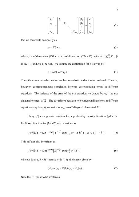
where y is of dimension ( TM × 1), X is of dimension ( TM × K)
, with K = ∑ i=
1 Ki
, β
is ( K × 1) and e is ( TM × 1) . We assume the distribution for e is given by
M
e~ N(0, Σ⊗ I T )
(4)
Thus, the errors in each equation are homoskedastic and not autocorrelated. There is,
however, contemporaneous correlation between corresponding errors in different
equations. The variance of the error of the i-th equation we denote by σ ii,
the i-th
diagonal element of Σ . The covariance between two corresponding errors in different
equations (say i and j), we write as σ ij,
an off-diagonal element of Σ .
Using f (.) as generic notation for a probability density function (pdf), the
likelihood function for
β and Σ can be written as
−MT
2 −T
2 1
−1
′
2
f( y| β, Σ ) = (2 π) Σ exp{ − ( y− Xβ) ( Σ ⊗I )( y− Xβ )} (5)
T
This pdf can also be written as
−MT
2 −T
2 1 −1
A
2
f( y| βΣ , ) = (2 π) Σ exp{ − tr( Σ )}
(6)
where A is an ( M × M)
matrix with ( i, j)
-th element given by
[ A] = ( y − X β )( ′ y − X β )
(7)
ij i i i j j j
Note that A can also be written as