Comparison of Observed Temperature and Salinity Changes in the ...
Comparison of Observed Temperature and Salinity Changes in the ...
Comparison of Observed Temperature and Salinity Changes in the ...

You also want an ePaper? Increase the reach of your titles
YUMPU automatically turns print PDFs into web optimized ePapers that Google loves.
1JANUARY 2003 BANKS AND BINDOFF<br />
163<br />
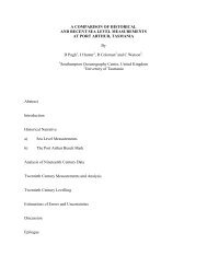
FIG. 7. Indo-Pacific zonal average <strong>in</strong> <strong>the</strong> HadCM3 model for <strong>the</strong> anthropogenic climate change<br />
scenario (B2) for (a) surface temperature change, (b) surface heat flux change, (c) surface sal<strong>in</strong>ity<br />
change, (d) surface freshwater <strong>in</strong>put (precipitation plus run<strong>of</strong>f m<strong>in</strong>us evaporation) change, (e)<br />
mean surface sal<strong>in</strong>ity, (f) zonal w<strong>in</strong>d stress change, <strong>and</strong> (g) Indo-Pacific zonal average potential<br />
temperature change on isopycnals regridded onto pressure surfaces, with zonal average sal<strong>in</strong>ity<br />
field shown <strong>in</strong> contours. The changes are differences between <strong>the</strong> averages <strong>of</strong> 1989–98 <strong>and</strong> 2019–<br />
28.<br />
duction, it is difficult from observations to piece toge<strong>the</strong>r<br />
changes <strong>in</strong> surface fluxes with changes <strong>in</strong> <strong>the</strong><br />
subsurface ocean properties, yet <strong>in</strong> <strong>the</strong> coupled model<br />
this should be possible. We will focus on <strong>the</strong> decades<br />
1989–98 <strong>and</strong> 2019–28 <strong>in</strong> B2. There are two reasons for<br />
do<strong>in</strong>g this: first, <strong>the</strong>se were <strong>the</strong> decades used <strong>in</strong> <strong>the</strong><br />
previous section to derive <strong>the</strong> f<strong>in</strong>gerpr<strong>in</strong>t; second, we<br />
expect <strong>the</strong> signal over this time period to have a higher<br />
signal-to-noise ratio than currently observed, <strong>and</strong> it<br />
should <strong>the</strong>refore be easier to deduce <strong>the</strong> l<strong>in</strong>ks between<br />
surface forc<strong>in</strong>g <strong>and</strong> <strong>the</strong> subsurface pattern.<br />
Figure 7a shows <strong>the</strong> zonal average change <strong>in</strong> surface<br />
temperature, which has <strong>in</strong>creased at all latitudes, except<br />
north <strong>of</strong> 65N. This suggests that <strong>the</strong> ocean has taken<br />
up heat. Figure 7b shows <strong>the</strong> zonal average change <strong>in</strong><br />
<strong>the</strong> surface heat flux. This does not reveal such a uniform<br />
pattern <strong>and</strong> is most likely to be <strong>the</strong> result <strong>of</strong> surface heat<br />
flux be<strong>in</strong>g a particularly noisy field. Although <strong>the</strong> surface<br />
heat flux field is very noisy <strong>the</strong> average surface<br />
flux change over <strong>the</strong> Indo-Pacific region is approximately<br />
0.4 W m 2 . For a swamp ocean 100 m thick,<br />
this heat flux over 30 yr would lead to a temperature<br />
change <strong>of</strong> 0.9C, or about twice <strong>the</strong> sea surface temperature<br />
change <strong>of</strong> <strong>the</strong> model (Fig. 7a). The average