Comparison of Observed Temperature and Salinity Changes in the ...
Comparison of Observed Temperature and Salinity Changes in the ...
Comparison of Observed Temperature and Salinity Changes in the ...

Create successful ePaper yourself
Turn your PDF publications into a flip-book with our unique Google optimized e-Paper software.
160 JOURNAL OF CLIMATE<br />
VOLUME 16<br />
FIG. 4. Potential temperature changes on isopycnals from HadCM3 anthropogenic climate<br />
change experiment (B2) (red) <strong>and</strong> observations (blue). Dashed l<strong>in</strong>es denote <strong>the</strong> error bars.<br />
<strong>the</strong> model <strong>and</strong> <strong>the</strong> observations. At 47N, both <strong>the</strong> observations<br />
<strong>and</strong> model show cool<strong>in</strong>g <strong>and</strong> freshen<strong>in</strong>g on<br />
isopycnals around <strong>the</strong> core <strong>of</strong> NPIW.<br />
c. Quantitative comparison <strong>of</strong> modeled <strong>and</strong> observed<br />
changes<br />
As we can see from Figs. 2 <strong>and</strong> 3, it is not straightforward<br />
to make a quantitative comparison <strong>of</strong> observed<br />
<strong>and</strong> modeled water mass changes on isopycnals because<br />
<strong>of</strong> <strong>the</strong> different absolute properties <strong>of</strong> water masses.<br />
However, because we can clearly identify <strong>the</strong> same water<br />
masses <strong>in</strong> both <strong>the</strong> observations <strong>and</strong> model, we believe<br />
that it is worthwhile to make a quantitative comparison<br />
<strong>of</strong> changes <strong>in</strong> each water mass. The method we<br />
have employed is new <strong>and</strong> <strong>in</strong>novative, but <strong>the</strong> <strong>in</strong>spiration<br />
came from <strong>the</strong> application <strong>of</strong> fuzzy logic (Guiot<br />
et al. 1999). The idea beh<strong>in</strong>d <strong>the</strong> approach is to look<br />
for similarities between pr<strong>of</strong>iles <strong>and</strong> allow some <strong>of</strong>fset<br />
<strong>in</strong> <strong>the</strong> positions <strong>of</strong> similar features.<br />
For both <strong>the</strong> model <strong>and</strong> <strong>the</strong> observations, we can def<strong>in</strong>e<br />
a potential temperature change on isopycnals, (),<br />
where is <strong>the</strong> potential temperature change <strong>and</strong> is<br />
<strong>the</strong> potential density. If we compare <strong>the</strong> observed change,<br />
obs (), with <strong>the</strong> modeled change at <strong>the</strong> same density,<br />
mod(),<br />
<strong>the</strong> comparison will be mean<strong>in</strong>gless because water<br />
masses are at different densities <strong>in</strong> <strong>the</strong> model <strong>and</strong> <strong>the</strong><br />
observations. To make a mean<strong>in</strong>gful comparison, we will<br />
<strong>in</strong>terpolate obs<br />
<strong>and</strong> mod onto a new ‘‘water mass axis’’<br />
that we will now def<strong>in</strong>e. In Table 2 we def<strong>in</strong>ed <strong>the</strong> pr<strong>in</strong>cipal<br />
water masses for each section <strong>in</strong> <strong>the</strong> model <strong>and</strong> <strong>the</strong><br />
observations (surface, sal<strong>in</strong>ity maximum, AAIW/NPIW,<br />
<strong>and</strong> deep water). For <strong>the</strong> Sou<strong>the</strong>rn Hemisphere sections<br />
<strong>the</strong>re are four water masses (n wm 4), while for <strong>the</strong><br />
Nor<strong>the</strong>rn Hemisphere sections <strong>the</strong>re are three water masses<br />
(n wm 3). We will call <strong>the</strong> water mass, wm(i), where<br />
i 0···n wm 1. The density <strong>of</strong> water mass, wm(i),<br />
<strong>in</strong> <strong>the</strong> observations is obs [wm(i)] <strong>and</strong> <strong>in</strong> <strong>the</strong> model is<br />
mod [wm(i)]. So for each water mass we can compare<br />
obs{ obs [wm(i)]} with mod{ mod [wm(i)]}.<br />
We can now take this one step fur<strong>the</strong>r <strong>and</strong> <strong>in</strong>terpolate<br />
<strong>the</strong> cont<strong>in</strong>uous pr<strong>of</strong>iles as a function <strong>of</strong> density to cont<strong>in</strong>uous<br />
pr<strong>of</strong>iles as a function <strong>of</strong> water mass. We def<strong>in</strong>e<br />
a water mass coord<strong>in</strong>ate, l, to lie between 0 <strong>and</strong> (n wm<br />
1), where is a ‘‘resolution factor.’’ Here we will<br />
take to be equal to 10. We chose this value <strong>of</strong> <br />
because this gave a resolution comparable with <strong>the</strong> orig<strong>in</strong>al<br />
data. Here l is def<strong>in</strong>ed as<br />
l i j, (1)<br />
where i 0...n wm 2 <strong>and</strong> j 0.... We can <strong>the</strong>n<br />
calculate <strong>the</strong> density at a particular l as<br />
j{[wm(i 1)] [wm(i)]}<br />
(l) [wm(i)] . (2)<br />
<br />
The potential temperature change at water mass coord<strong>in</strong>ate<br />
l is <strong>the</strong>n simply [(l)]. We can <strong>the</strong>n make a<br />
comparison between <strong>the</strong> observations <strong>and</strong> <strong>the</strong> model by<br />
compar<strong>in</strong>g obs[ obs (l)] with mod[ mod (l)].<br />
Figure 4 shows <strong>the</strong> potential temperature changes on<br />
isopycnals plotted aga<strong>in</strong>st a water mass axis from both<br />
<strong>the</strong> model <strong>and</strong> observations. We have <strong>in</strong>cluded error bars