Comparison of Observed Temperature and Salinity Changes in the ...

156 JOURNAL OF CLIMATE
VOLUME 16
Comparison of Observed Temperature and Salinity Changes in the Indo-Pacific with
Results from the Coupled Climate Model HadCM3: Processes and Mechanisms*
HELENE T. BANKS
Hadley Centre for Climate Prediction and Research, Met Office, Bracknell, Berkshire, United Kingdom
NATHANIEL L. BINDOFF
Antarctic Co-operative Research Centre, Hobart, Australia
(Manuscript received 28 December 2001, in final form 2 July 2002)
ABSTRACT
Observed changes in temperature and salinity properties on isopycnals across hydrographic sections throughout
the Indo-Pacific are compared with the changes modeled by the coupled climate model, HadCM3. Observations
show cooling and freshening on isopycnals in midlatitudes, and there is quantitative agreement between modeled
and observed water mass changes on five out of six zonal sections. The full Indo-Pacific pattern of change in
the climate model is examined and it is discovered that the pattern of cooling and freshening on isopycnals in
midlatitudes, with warming on isopycnals at high latitudes, may be thought of as a fingerprint of anthropogenic
forcing. The water mass changes are related to changes in the surface fluxes and it is found that surface warming
is the dominant factor in producing water mass changes, although changes in the freshwater cycle are important
in the formation zone for Antarctic Intermediate Water. The coupled model has a low-amplitude, low-frequency
(100-yr period) internal mode related to the anthropogenic fingerprint. Further observations are required to
measure the amplitude of the internal mode as well as the anthropogenically forced mode.
1. Introduction
Over the last 40 years there have been a number of
observations of temperature and salinity properties of
subsurface water masses in the Indo-Pacific (Bindoff
and Church 1992; Johnson and Orsi 1997; Wong et al.
1999; Bindoff and McDougall 2000). These observations
show that in mode and intermediate waters, the
water mass properties have become colder and fresher
on isopycnals over this period. Changes in temperature
and salinity on isopycnals reflect changes in surface
forcing, yet it may be extremely difficult to link observed
subsurface changes with observed changes in
surface forcing. Inherent noise and natural variability
of the ocean surface makes direct measurements of surface
fluxes difficult and, as a consequence, measurements
of long-term changes in surface fluxes are affected
by low signal-to-noise ratios. Subsurface ocean
temperature and salinity fields can act to integrate sur-
* This study contributes to the World Ocean Circulation Experiment.
Corresponding author address: Dr. Helene T. Banks, Hadley Centre
for Climate Prediction and Research, Met Office, London Road,
Bracknell, Berkshire RG12 2SY, United Kingdom.
E-mail: helene.banks@metoffice.com
face fluxes and because of relatively low variability in
the subsurface ocean (as shown by Banks and Wood
2002), high signal-to-noise ratios should be found there.
There has been much speculation about whether the
observed changes are a natural cycle of the climate system
or forced by anthropogenic climate change (Wong
et al. 1999), but, given that subsurface ocean measurements
only go back approximately 60 years (Levitus et
al. 1998), it is virtually impossible to ascertain this from
ocean observations themselves.
Coupled ocean–atmosphere models have become sufficiently
sophisticated in the last five years that artificial
flux adjustments that may have hindered their realism
are now no longer necessary (Gordon et al. 2000). These
models are now producing simulations of the last century
based on historical records of atmospheric constituents
with projections into the future based on scenarios
and are used to give policy advice through the
Intergovernmental Panel on Climate Change (IPCC)
process (Houghton et al. 2001). In order to establish the
credibility of models such as these, it is important to
validate their simulations of the last century against observed
historical changes in the climate system, both in
the atmosphere and the ocean. Levitus et al. (2001) and
Barnett et al. (2001) have shown that two coupled models
can produce observed trends in ocean heat content.
Our work aims to look at whether one coupled model

1JANUARY 2003 BANKS AND BINDOFF
157
TABLE 1.
Zonal
section
47N
24N
10N
17S
32S
43S
Modern and historical data used in the comparison.
Modern
(yr)
1985
1985
1989
1994
1987
1989
No. of
casts
299
156
213
294
109
72
Historical
(yr)
1966
1970
1969
1967
1962
1967
No. of
casts
299
509
400
706
451
18
Std dev
(yr)
5.0
5.5
6.0
5.0
10.0
1
Time
difference
(yr)
19
15
20
30
25
22
can produce the observed changes in temperature and
salinity on isopycnals. Beyond validation, in a coupled
model it is possible to diagnose surface forcing and,
therefore, to try to understand the processes and mechanisms
by which subsurface oceanic changes may occur.
This paper aims to address three questions: 1) Can a
coupled climate model reproduce observed water mass
changes in the Indo-Pacific? 2) Are observed changes
anthropogenically forced or a signal of internal variability?
3) What atmospheric changes drive the observed
subsurface water mass changes? We will first
describe observations from the Indo-Pacific over the last
century and simulations of a state-of-the-art coupled
climate model, the third Hadley Centre Coupled Ocean–
Atmosphere General Circulation Model (HadCM3; section
2). We will then compare observed changes in temperature
and salinity with those simulated by the coupled
climate model (section 3). In section 4 we will find
the pattern of change in the coupled model that may be
thought of as a fingerprint of anthropogenic forcing, and
in section 5 we will relate the subsurface fingerprint to
the changes in surface fluxes. Finally, in section 6 we
will draw conclusions.
2. Data and methods
a. The data
We compare the output of the model with the observed
differences in temperature and salinity in the
deep ocean (Table 1). These differences are constructed
from a variety of datasets and analyses (Bindoff and
Church 1992; Bindoff and McDougall 1994, 2000;
Wong et al. 2001). The historical data are primarily
obtained from J. Reid and A. Mantyla (1994, personal
communication) and from the Southern Ocean Atlas
(Gordon et al. 1982) for both the Indian and Pacific
Oceans. The hydrographic data from these atlases are
mainly Nansen bottle data. The recent hydrographic data
come from the World Ocean Circulation Experiment
(WOCE) and are available from the World Hydrographic
Program Office (WHPO; see online at http://
whpo.ucsd.edu). These WOCE data are all CTD data
calibrated against salinity analyses from water samples
taken through the whole water column. Typical accuracies
of the CTD temperature and salinity data are
0.002C and 0.003 psu. The historical data are interpolated
to the location of each cast from the recent
hydrographic profiles using objective methods (Bretherton
et al. 1976; Roemmich 1983; Bindoff and Wunsch
1992). The observed differences along these sections
(Table 1) are distributed over both the Pacific and Indian
Oceans (Fig. 1). The best coverage is of the Pacific
basin, although the South Pacific is less well covered.
These observed differences have been interpreted in earlier
papers (listed above) but are now compared with
the HadCM3 model for the first time.
FIG. 1. The locations of the historical and modern data used to compare with the results from
the coupled ocean–atmosphere model (HadCM3).

158 JOURNAL OF CLIMATE
VOLUME 16
b. Numerical model
The model we will look at here is the coupled ocean–
atmosphere model, HadCM3 (Gordon et al. 2000), developed
at the Hadley Centre. The major differences
between this coupled model and the previous version
(Johns et al. 1997) occur in the ocean component, which
has higher horizontal resolution and employs the Gent
and McWilliams (1990) scheme to represent mixing due
to eddies. The introduction of these and other improvements
meant that the coupled model no longer needed
artificial flux adjustments to prevent the model drifting
to an unrealistic state and exact fluxes are exchanged
between the atmosphere and the ocean on a daily basis.
The ocean component of the model is based on the Cox
(1984) model with a horizontal resolution of 1.25 in
both the north–south and east–west direction and 20
vertical levels. The reader is referred to Gordon et al.
(2000) for details of the model.
Here we will examine two experiments; firstly, the
control experiment (CTL) and secondly an anthropogenic
climate change experiment B2. CTL is initialized
with the temperature and salinity of the ocean given by
the climatology of Levitus and Boyer (1994) and with
both the atmosphere and ocean at rest. While the oceanic
and atmospheric heat budgets come into balance within
10 yr in CTL (Gordon et al. 2000), this is not the case
for the freshwater budgets, which require a timescale of
the order of 300–400 yr to come into balance (Pardaens
et al. 2001, manuscript submitted to Climate Dyn., hereafter
PBGR). Since any imbalance will directly affect
the salinity structure of the ocean, this means that the
water mass properties must have a similar timescale to
the salinity field to reach a quasi equilibrium. For this
reason, in this paper we will only look at water mass
properties from year 370 onward.
Experiment B2 is initialized at year 370 of CTL. The
B2 is a climate change experiment with imposed anthropogenic
changes of well-mixed greenhouse gases,
tropospheric and stratospheric ozone and sulphate aerosols,
and is described in detail by Johns et al. (2001).
The B2 is forced using historical emissions and concentrations
from 1859 until the present, then the IPCC
B2 scenario until 2100. Experiment B2 has previously
been used by Banks et al. (2000) and Banks and Wood
(2002) to look at changes in water mass properties. A
simpler experiment with HadCM3 based on 2% increase
per year in carbon dioxide was used by Banks et al.
(2002) to understand the causes of change in Subantarctic
Mode Water in the Indian Ocean. The present
paper is the first to quantitatively compare HadCM3 and
observations throughout the Indo-Pacific and in its examination
of the basinwide modes of the Indo-Pacific.
FIG. 2. Temperature–salinity diagrams showing the Southern Hemisphere
section average water mass changes found in both (a), (c), (e)
the observations and (b), (d), (f) in the HadCM3 anthropogenic climate
change experiment (B2) of HadCM3 for the period shown in
Table 1. (a), (b): 17S; (c), (d): 32S; and (e), (f): 43S. The continuous
lines are the old water mass characteristics, and the dashed lines are
the new characteristics. The reader is referred to Fig. 4 to examine
the changes in detail.
3. Comparison of observed changes and coupled
model changes
a. Qualitative comparison of modeled and observed
temperature–salinity properties
Figure 1 shows the location of the observations used
in this study (Wong et al. 1999). The dates of the observations
are described in Table 1. It should be noted
that the historical data are interpolated onto the location
of the modern sections and have an associated error bar
to account for the effects of mesoscale variability. We
will use the uncertainties later. For the model data we
have extracted zonal sections from the annual means of
the years of the historical and modern observations at
the same latitudes as the observed sections. We have
calculated error bars for the model to account for the
uncertainty in the date of the historical data and shortterm
variability of the model. This is based on the standard
deviation of 5-yr differences in B2.
Figure 2 shows temperature–salinity diagrams from
both the modern and historical times for both the observational
data and the modeled data at the three southern
sections; 43, 32, and 17S. The bold lines denote
the historical temperature–salinity profile, while the
dashed lines denote the modern profile. In each case,
the modeled and observed temperature–salinity profiles
are qualitatively similar; in each profile there is a well-

1JANUARY 2003 BANKS AND BINDOFF
159
TABLE 2. Potential density (kg m 3 ) of water masses in both model
and observations. Note that for the section at 47N we take surface
to be the upper limit of the zone of almost homogeneous salinity (see
Figs. 3a and 3b).
Section Water mass Observed Modeled
43S
32S
17S
10N
24N
47N
Surface
Salinity max
AAIW
Deep
Surface
Salinity max
AAIW
Deep
Surface
Salinity max
AAIW
Deep
Surface
NPIW
Deep
Surface
NPIW
Deep
Surface
NPIW
Deep
23.2
26.6
27.4
28.0
23.2
26.0
27.4
28.0
23.2
24.4
27.0
27.8
23.2
27.2
28.0
23.2
26.8
27.8
24.0
26.4
27.8
24.8
25.4
26.2
28.0
22.8
24.8
26.4
28.0
20.9
24.4
26.2
28.0
21.4
26.4
27.8
23.1
25.2
27.8
24.8
25.6
27.8
FIG. 3. The Northern Hemisphere average water mass changes
found in both (a), (c), (e) the observations and (b), (d), (f) in the
HadCM3 anthropogenic climate change experiment (B2) of HadCM3
for the period shown in Table 1. (a), (b): 47N; (c), (d): 24N; and
(e), (f): 10N. The continuous lines are the old water mass characteristics,
and the dashed lines are the new characteristics. The reader
is referred to Fig. 4 to examine the changes in detail.
defined salinity minimum denoting Antarctic Intermediate
Water (AAIW). In the observations the minimum
occurs at approximately 34.5 psu, 5C, while in the
model the minimum occurs at approximately 34 psu,
9C. In both the observations and the model, below the
salinity minimum, salinity increases to deep water (before
decreasing in bottom water), while above the salinity
minimum, salinity increases to reach a maximum
before decreasing to the surface. For each section, Table
2 shows the density of the four water masses [surface,
salinity maximum, AAIW (salinity minimum), and deep
water] in both the observations and the model. The temperature–salinity
diagrams are not quantitatively similar
because in the coupled model, the ocean adjusts to balance
the surface fluxes given by the atmospheric model.
In the upper 1000 m, it takes about 400 yr for the temperature
and salinity properties to reach a quasi equilibrium.
Fortunately the observed and modeled temperature–salinity
(T–S) diagrams are qualitatively similar,
so we can still compare the water masses.
Figure 3 shows similar diagrams for the northern sections.
At 10N, the observations show a salinity minimum
associated with North Pacific Intermediate Water
(NPIW) at 34.5 psu, 6C, while the model has a salinity
minimum at 33.8 psu, 9C. At 24N, the salinity minimum
is at 34.1 psu, 7C in the observations and 33.7
psu, and 13C in the model. At 47N, both the modeled
and observed temperature–salinity diagrams have a different
shape to profiles farther south. This is because at
this latitude we are in the center of the formation region
for NPIW. This is identifiable by the ‘‘corner’’ in the
T–S profile. This corner occurs at 33.3 psu, 4C in the
observations, and 32.5 psu, 5C in the model. The densities
of the significant water masses in the northern
sections are also shown in Table 2.
b. Qualitative comparison of modeled and observed
changes
From Fig. 2 we can see that at 43S, in both the
observations and the model, the water masses above
AAIW became colder and fresher along isopycnals. A
similar freshening occurs at 32S, with waters at the
shallow salinity maximum becoming warmer and saltier
on isopycnals. At 17S, although the observed changes
seem fairly small, compared to the modeled changes,
we can see a similar pattern emerging from both the
model and the observations around AAIW.
In the Northern Hemisphere (Fig. 3), we can see subtropical
waters becoming warmer and saltier on isopycnals
at 10N while NPIW becomes colder and fresher.At24N,
NPIW becomes colder and fresher in the
observations and warmer and saltier in the model, while
subtropical waters become colder and fresher in both

160 JOURNAL OF CLIMATE
VOLUME 16
FIG. 4. Potential temperature changes on isopycnals from HadCM3 anthropogenic climate
change experiment (B2) (red) and observations (blue). Dashed lines denote the error bars.
the model and the observations. At 47N, both the observations
and model show cooling and freshening on
isopycnals around the core of NPIW.
c. Quantitative comparison of modeled and observed
changes
As we can see from Figs. 2 and 3, it is not straightforward
to make a quantitative comparison of observed
and modeled water mass changes on isopycnals because
of the different absolute properties of water masses.
However, because we can clearly identify the same water
masses in both the observations and model, we believe
that it is worthwhile to make a quantitative comparison
of changes in each water mass. The method we
have employed is new and innovative, but the inspiration
came from the application of fuzzy logic (Guiot
et al. 1999). The idea behind the approach is to look
for similarities between profiles and allow some offset
in the positions of similar features.
For both the model and the observations, we can define
a potential temperature change on isopycnals, (),
where is the potential temperature change and is
the potential density. If we compare the observed change,
obs (), with the modeled change at the same density,
mod(),
the comparison will be meaningless because water
masses are at different densities in the model and the
observations. To make a meaningful comparison, we will
interpolate obs
and mod onto a new ‘‘water mass axis’’
that we will now define. In Table 2 we defined the principal
water masses for each section in the model and the
observations (surface, salinity maximum, AAIW/NPIW,
and deep water). For the Southern Hemisphere sections
there are four water masses (n wm 4), while for the
Northern Hemisphere sections there are three water masses
(n wm 3). We will call the water mass, wm(i), where
i 0···n wm 1. The density of water mass, wm(i),
in the observations is obs [wm(i)] and in the model is
mod [wm(i)]. So for each water mass we can compare
obs{ obs [wm(i)]} with mod{ mod [wm(i)]}.
We can now take this one step further and interpolate
the continuous profiles as a function of density to continuous
profiles as a function of water mass. We define
a water mass coordinate, l, to lie between 0 and (n wm
1), where is a ‘‘resolution factor.’’ Here we will
take to be equal to 10. We chose this value of
because this gave a resolution comparable with the original
data. Here l is defined as
l i j, (1)
where i 0...n wm 2 and j 0.... We can then
calculate the density at a particular l as
j{[wm(i 1)] [wm(i)]}
(l) [wm(i)] . (2)
The potential temperature change at water mass coordinate
l is then simply [(l)]. We can then make a
comparison between the observations and the model by
comparing obs[ obs (l)] with mod[ mod (l)].
Figure 4 shows the potential temperature changes on
isopycnals plotted against a water mass axis from both
the model and observations. We have included error bars

1JANUARY 2003 BANKS AND BINDOFF
161
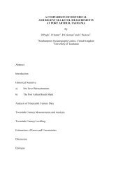
FIG. 5. Indo-Pacific zonal average potential temperature change on isopycnals from HadCM3
anthropogenic climate change experiment (B2) between 1959–68 and 1989–98. The changes on
isopycnals have been regridded onto pressure surfaces using the mean depth of each isopycnal
surface. Contours show the zonal average salinity field.
(as mentioned earlier) on both the modeled and observed
changes. At 43 and 32S, both the model and observations
show cooling between AAIW and the salinity
maximum. This is the part of the water column where
Subantarctic Mode Water (SAMW) is found. At these
latitudes the observed and modeled changes are of a
similar magnitude. At 17S, the observations show a
weak cooling (approximately 0.1C) around the salinity
minimum associated with AAIW, while the modeled
cooling is approximately 0.5C and higher in the water
column, around the salinity maximum (this difference
can also be seen in Fig. 2). The difference between the
model and observations cannot be explained by mesoscale
or interannual variability as it lies outside the error
bars of both the model and observations. In the Northern
Hemisphere, although the changes at 10N are weak in
both the model and the observations, there is general
agreement between the two. At 24N, the comparison
shows differences in the direction of the changes but
the interannual variability (as shown by the model error
bars) is large enough to contribute toward this difference
except at depth. At 47N, the observations and the model
both show cooling of a similar magnitude through the
water column.
In summary, for five out of six sections there is quantitative
agreement between the changes in the modeled
and observed water masses, which suggests that the
model is capable of simulating the observed large-scale
pattern of change.
4. The fingerprint of anthropogenic forcing in the
Indo-Pacific
In the previous section we showed that the coupled
model is able to capture the large-scale signal of cooling
and freshening on isopycnals over the last 30 yr, as seen
in the observations. In this section we aim to use the
coupled model to see if the pattern we have seen is a
signal of anthropogenic climate change or whether it is
simply part of the internal variability of the climate
system.
Figure 5 shows the zonally averaged change in temperature
on isopycnals for the Indo-Pacific between the
decadal means of 1959–68 and 1989–98 in the anthropogenic
climate change (B2) model run. We choose a
30-yr period because this is a timescale typical of the
separation time for observations (as seen in Table 1).
By taking the difference of decadal averages we can
eliminate variability on the interannual timescale. It
shows that the water column has become warmer (and
saltier) at high latitudes (poleward of 45). Cooling (and
freshening) originates from the surface in the Southern
Hemisphere subtropics and extends below the surface
into the Northern Hemisphere. In the Tropics the surface
becomes warmer (and saltier) and in the Northern Hemisphere
subtropics the water column has also become
warmer (and saltier). In the Southern Hemisphere this
pattern is similar to that shown by the earlier model–
data comparison. In addition, although changes in the
high latitudes have been poorly sampled in the observations,
there is evidence to suggest that warming on
isopycnals, as seen in the coupled model, is occurring
(Aoki 1997; Aoki et al. 2001, manuscript submitted to
J. Geophys. Res.). In the Northern Hemisphere the pattern
is somewhat different to that seen earlier with less
cooling and freshening apparent. This underlines the
larger interannual and interdecadal variability in the
Northern Hemisphere compared to the Southern Hemisphere,
as suggested by the results of Banks et al. (2000).
We call the pattern of change described above the asymmetric
pattern and examine both CTL and B2 to see
whether it is a signal of anthropogenic change.

162 JOURNAL OF CLIMATE
VOLUME 16
We take the asymmetric pattern shown in Fig. 5 to
be P(x), where x 1...n is the position in latitude–
depth space. From the CTL run we will take the time
series of every (overlapping) 30-yr zonal average Indo-
Pacific change of salinity on isopycnals. The differences
are created by shifting the 30-yr period by 1 yr at a
time. Since temperature and salinity changes on isopycnals
are compensating it does not matter whether we
choose to look at temperature or salinity. This is a representation
of the changes due to internal variability of
the coupled system. We will call this time series I(x, t),
where t denotes the time of the first year in the 30-yr
difference. In addition, we will also take from B2 the
time series of every 30-yr zonal average Indo-Pacific
change of salinity on isopycnals. This is a representation
of the changes due to anthropogenic forcing and we will
call this time series A(x, t).
We will then project both our time series of differences
[I(x, t) and A(x, t)] onto the asymmetric pattern
[P(x)] to create time series u(t) and (t) (see, e.g., Santer
et al. (1995). These time series are calculated:
n
I(x, t)P(x) x1
u(t)
n
(3)
P(x)P(x) x1
n
A(x, t)P(x) x1
(t)
n
. (4)
P(x)P(x) x1
Figure 6a shows u as a function of time. The internal
variability u shows no significant drift over time and
has periods that are correlated and anticorrelated with
the asymmetric pattern but is essentially a random time
series. Based on a one-tailed test (since we are looking
for a positive correlation with the search pattern), the
5% significance level in the distribution of u is 0.5 (the
time series has 31 degrees of freedom). This value is
highlighted in Fig. 6a. The time series of (Fig. 6b)
shows that before 1950 there is no strong correlation
with the asymmetric pattern. After 1950 the anthropogenic
changes show a much redder spectrum with distinct
periods of correlation with the asymmetric pattern;
starting in approximately 1960, 2000, and 2050. Examining
the time series of u and suggests that CTL
has no significant correlation with the asymmetric pattern
and while the pattern becomes more common as
anthropogenic forcing increases it is not dominant. To
try and establish what pattern occurs when the projected
values are low we will look at the 30-yr difference pattern
starting in the 1990s.
Figure 7g shows the zonally averaged change in temperature
on isopycnals between the decadal means of
1989–98 and 2019–28 from the anthropogenic climate
change run (B2). This shows a pattern similar in many
FIG. 6. Time series of the correlation of 30-yr changes in (a) CTL
and (b) B2 projected onto the difference pattern from 1989 to 1998
minus 1959 to 1968. The 5% significance level from the CTL distribution
is marked as the dashed line in both (a) and (b). Please note
the different time axis in (a) and (b).
ways to that seen in Fig. 5 but with greater symmetry
between the Northern and Southern Hemispheres and,
in particular, cooling (and freshening) of the water column
in the northern subtropics. We will call this the
symmetric pattern and note that this pattern is qualitatively
very similar to that seen in the observations. If
we now repeat the projection of all the 30-yr differences
onto the symmetric pattern, we get a somewhat different
picture. Figure 8a shows that in the internal variability
of the coupled system this pattern (although weak) does
show some signs of low-frequency variability with a
timescale of approximately 100 yr. Figure 8b shows,
however, that the symmetric pattern is the dominant
signal of anthropogenic forcing in the Indo-Pacific; all
30-yr changes starting from about 1960 exceed the 5%
significance level from the internal variability. This suggests
that the large-scale pattern of change seen in the
observations of cooling and freshening on isopycnals
in the subtropics of both hemispheres with warming
(and salinification) occurring near the surface, may be
thought of as a fingerprint of anthropogenic climate
change in the ocean.
5. Mechanisms for the fingerprint
In this section we will focus on the fingerprint pattern
seen in the coupled model. As discussed in the intro-

1JANUARY 2003 BANKS AND BINDOFF
163
FIG. 7. Indo-Pacific zonal average in the HadCM3 model for the anthropogenic climate change
scenario (B2) for (a) surface temperature change, (b) surface heat flux change, (c) surface salinity
change, (d) surface freshwater input (precipitation plus runoff minus evaporation) change, (e)
mean surface salinity, (f) zonal wind stress change, and (g) Indo-Pacific zonal average potential
temperature change on isopycnals regridded onto pressure surfaces, with zonal average salinity
field shown in contours. The changes are differences between the averages of 1989–98 and 2019–
28.
duction, it is difficult from observations to piece together
changes in surface fluxes with changes in the
subsurface ocean properties, yet in the coupled model
this should be possible. We will focus on the decades
1989–98 and 2019–28 in B2. There are two reasons for
doing this: first, these were the decades used in the
previous section to derive the fingerprint; second, we
expect the signal over this time period to have a higher
signal-to-noise ratio than currently observed, and it
should therefore be easier to deduce the links between
surface forcing and the subsurface pattern.
Figure 7a shows the zonal average change in surface
temperature, which has increased at all latitudes, except
north of 65N. This suggests that the ocean has taken
up heat. Figure 7b shows the zonal average change in
the surface heat flux. This does not reveal such a uniform
pattern and is most likely to be the result of surface heat
flux being a particularly noisy field. Although the surface
heat flux field is very noisy the average surface
flux change over the Indo-Pacific region is approximately
0.4 W m 2 . For a swamp ocean 100 m thick,
this heat flux over 30 yr would lead to a temperature
change of 0.9C, or about twice the sea surface temperature
change of the model (Fig. 7a). The average

164 JOURNAL OF CLIMATE
VOLUME 16
FIG. 8. Time series of the correlation of 30-yr changes in (a) CTL
and (b) B2 projected onto the difference pattern from 2019 to 2028
minus 1989 to 1968. The 5% significance level from the CTL distribution
is marked as the dashed line in both (a) and (b). Please note
the different time axis in (a) and (b).
surface heat flux change implies a change in heat content
of 9 10 22 J over the Indo-Pacific region. The actual
heat content change over the region is 16 10 22 J. This
difference cannot be accounted for by changes in the
heat transported into the Indo-Pacific (this actually decreases
by 0.02 PW). The discrepancy therefore implies
that the time-integrated surface heat flux increase is actually
larger than estimated by the differences between
two periods (giving an average of 0.68 W m 2 over the
Indo-Pacific). The uniformity of the sea surface temperature
field (relative to the driving heat flux field)
demonstrates the strong integrating response of the
ocean to atmospheric forcing.
Similarly the ocean is a strong integrator of changes
in precipitation. Figure 7c shows the zonal average
change in surface salinity. The salinity changes shows
freshening at all latitudes (except near 30S). Figure 7d
shows the zonal average change in surface freshwater
input from precipitation, runoff, and evaporation. Precipitation
(and runoff) has increased at high (poleward
of 45) and low (equatorward of 10) latitudes, while
evaporation has increased in midlatitudes in both hemispheres.
As for temperature, it is not straightforward to
draw parallels between changes in surface fluxes and
changes in surface properties. In midlatitudes it may be
the case that, as seen in the adjustment of CTL (PBGR),
when the surface becomes warmer or fresher, greater
stability inhibits vertical mixing (both wind driven and
convective mixing). In this manner the surface properties
will tend to be dominated by warming and freshening
rather than cooling and salinification. Surface salinity
(and temperature) may also be affected by changes
in winds through changes in the surface Ekman transport
as suggested by Rintoul and England (2002). Figure 7e
shows the zonal surface salinity and hence its gradients.
Northward Ekman transport is proportional to x / f,
where x is the zonal wind stress and f is the Coriolis
parameter. Increases in the zonal wind stress lead to an
increase in equatorward Ekman transport. Figure 7f
shows that there is an increase in the zonal wind stress
in the Southern Hemisphere between 50 and 30S,
which drives fresher water into midlatitudes, while in
the Northern Hemisphere there is an increase in zonal
wind stress north of 45N, which drives fresher water
southward. Similarly, south of 50S the zonal wind
stress has decreased leading to a southward Ekman
transport driving fresher surface waters to the north
southward. Combined with the increase in precipitation
minus evaporation (P E) the surface waters in this
region give a net decrease in salinity. The surface salinity
signal at all latitudes ranges (except between 12
and 45N) can be explained by the balance of Ekman
transport of the preexisting surface salinity gradient and
the changes in precipitation plus runoff minus evaporation.
Having examined the modeled changes in surface
fluxes and the modeled change in subsurface properties,
leads us to ask whether the two fit together to give a
consistent picture. To do this we need to think about
what combination of surface forcing can produce changes
on isopycnals. If the water column is salty near the
surface and fresher below (assuming that temperature
is stably stratified), then adding cold or salty water at
the surface will lead to warming on isopycnals. Alternatively,
adding warm or freshwater at the surface will
lead to cooling on isopycnals. If the water column is
fresh near the surface and saltier below, then adding
cold or freshwater at the surface will lead to cooling on
isopycnals, while adding warm or salty water at the
surface will lead to warming on isopycnals. The reader
is referred to Figs. 1 and 2 from Bindoff and McDougall
(1994) for further insight into these changes.
In the model we see warming on isopycnals south of
51S (e.g., Figs. 5 and 7g). The water column is fresher
near the surface and the –S diagram has a negative
slope. Because the surface waters have both warmed
and freshened the new near-surface –S curve is now
displaced upward. On isopycnals, the temperature (and
salinity) now appear warmer (and paradoxically saltier).
For more detailed discussion of this response to changed
surface waters see Bindoff and McDougall (1994). The
precise contribution from the freshening and warming

1JANUARY 2003 BANKS AND BINDOFF
165
of the surface waters can be solved using the methods
of Bindoff and McDougall (1994, 2000).
Between 42 and 51S, the –S relation still has a
negative slope (i.e., just south of the core of the salinity
minimum). However, the surface water properties are
different. The surface temperature change is small in
this latitude band (0.1C), while the surface salinity
change is relatively large driven mainly by the large
surface precipitation increase here. The increase in surface
salinity displaces the –S curve downward (and to
the left). On isopycnals the temperature (salinity)
change is toward cooling and (freshening). This zone
is the formation zone for Antarctic Intermediate Waters
(AAIW).
Between 28 and 42S the surface waters are warmer
and saltier than the waters below (–S diagram has positive
slope). The changes in surface water properties in
this latitude band are toward warmer (0.5C) water with
slightly increased surface salinity (0.005 psu). The
increase in surface temperature displaces the new –S
curve upward (and to the left). On isopycnals the temperature
(salinity) is now paradoxically cooler (and
fresher). This latitude band is the formation zone for
SAMW. In the Tropics, between 3 and 28S the –S
curve has a negative slope above the shallow salinity
maximum. The surface waters are much warmer
(0.25C) than the relatively weak salinity decrease.
Applying the same arguments as for south of 51S on
isopycnals the temperature (salinity) is now warmer
(saltier).
Using the same arguments as in the Southern Hemisphere,
in the Northern Hemisphere we see a similar
pattern of modeled changes on isopycnals being driven
by the changes in the surface water properties. Although
the surface salinity decreases are large in the North Pacific,
the surface temperature increases are also large
and tend to dominate the water mass changes. This is
because the North Pacific is a relatively warm ocean
and the thermal expansion coefficient is much larger
than the haline contraction coefficient. On a –S curve
this means that the temperature changes are always moving
the water mass properties farther along the temperature
axis than the salinity decreases are moving water
mass properties along the salinity axis.
The overall pattern of water mass change of the ocean
interior for the 30-yr period from 1989–98 to 2019–28
is warming driven by the warmed surface waters. The
only exception is the area in the formation zone of
AAIW water (between 51 and 43S), where the surface
temperature increase is small (in density terms) and
where the strong precipitation increase has made the
surface salinity decrease relatively strong.
6. Discussion
The aims of this paper were threefold; to evaluate the
response of the coupled model HadCM3 in the Indo-
Pacific over the last 40 yr in terms of temperature and
salinity changes, to understand which aspects of surface
forcing drive the response in the interior ocean and to
assess whether the large-scale pattern in the Indo-Pacific
is a signature of anthropogenic climate change or whether
it is simply a pattern that occurs as part of the internal
variability of the coupled system.
In order to evaluate the modeled changes in temperature
and salinity on isopycnals we developed a method
to compare changes on a water mass axis. This method
allowed a quantitative comparison to be made even
when the basic temperature–salinity diagrams were only
qualitatively the same. We envisage that this method
could be used in other model–data comparisons to move
toward quantitative evaluation of models. Using this
method we were able to see that out of six sections
throughout the Indo-Pacific, five of them showed good
agreement between the modeled and observed changes.
With just six sections, the emerging pattern was of a
symmetric pattern of cooling (and freshening) on isopycnals
in intermediate waters (i.e., salinity minimum
and mode waters) of both hemispheres with warming
on isopycnals near the surface.
The difficulties with looking at the changes on discrete
sections are that we do not have the whole picture
and the snapshot differences were taken at different
times for each latitude. In the model, when we looked
at the full two-dimensional picture of the changes between
two decades (1959–68 and 1989–98) we saw a
slightly different picture emerging—one of asymmetry
between the two hemispheres—with the Southern Hemisphere
showing the pattern of cooling on isopycnals,
while the Northern Hemisphere is dominated by a pattern
of warming on isopycnals. The later hydrographic
sections at both 24 and 47N were taken several years
earlier than at more southerly latitudes (see Table 1) and
it is plausible that the warming pattern may have been
weaker at that stage in the Northern Hemisphere. In
HadCM3, the asymmetric pattern is more likely to occur
due to anthropogenic climate change but it is probably
not a pattern that will exclusively dominate. By looking
at a period when changes did not project strongly onto
the asymmetric pattern, we found a symmetric pattern
that, when projected onto the time series, appeared to
be dominant under anthropogenic forcing. The strong
similarity between the symmetric pattern and the observed
changes suggests that the observed pattern is
most likely to be a signature of anthropogenic climate
change. It is interesting to note, however, that unlike
our asymmetric pattern, the symmetric pattern did show
signs of a weak low-frequency variability in the internal
variability with a timescale of approximately 100 yr. If
the model does provide a good representation of the real
world, it may be the case that the phase of the symmetric
mode in the internal variability may be enhancing the
strength of the observed signal.
In the real world it is almost impossible to produce
a self-consistent picture relating observed interior
changes to observed surface fluxes. In a coupled model

166 JOURNAL OF CLIMATE
VOLUME 16
this should be possible, yet often it can still be difficult
to draw a coherent picture. In HadCM3 we have a picture
where surface warming dominates the subsurface
response at almost all latitudes except in the formation
zone for Antarctic Intermediate Water where surface
freshening (due to increased precipitation) is also important.
Wind stress changes through Ekman transport
are also important for driving changes in surface salinity.
In conclusion, the coupled model HadCM3 can simulate
with reasonable skill interior ocean changes observed
over the last 40 yr. The challenge for the future
is to produce a dataset which is less limited in both
spatial and temporal extent to further test coupled model
simulations. In the case of the Indo-Pacific, our biggest
uncertainty in the coupled model is in the response of
the North Pacific. Further observations may help to
characterize the interannual and interdecadal variability
in that basin. We have shown that a symmetric pattern
of warming on isopycnals at high latitudes and cooling
on isopycnals at midlatitudes may be thought of as a
fingerprint of anthropogenic forcing. Our biggest uncertainty
in relation to the observations is that in the
coupled model the symmetric pattern also occurred on
a 100-yr timescale as part of internal variability. One
caveat in our results is that we have only shown that
this mode appears in the coupled model. This does not
mean that this mode will necessarily appear in the real
world. If this mode is real and it were subsequently
found that the model estimate of internal variability is
too low, it then becomes plausible that the observed
water mass changes may be due to internal variability
of the coupled system. Further observations are needed
over the entire Indo-Pacific to monitor changes and assess
the level of variability produced by coupled models
used to predict changes in climate under anthropogenic
forcing. The requirement for continued subsurface
ocean observations may be partly met by the Argo project
(an array of profiling floats; Wilson 2000), but repeat
hydrographic sections may also be necessary to
supplement the floats.
Acknowledgments. We thank Annie Wong for the analyzed
hydrographic data from the Pacific Ocean and
two reviewers for their comments. The work of HTB
was carried out under DEFRA Contract PECD 7/12/37.
REFERENCES
Aoki, S., 1997: Trends and interannual variability of surface layer
temperature in the Indian sector of the Southern Ocean observed
by the Japanese Antarctic Research Expeditions. J. Oceanogr.,
53, 623–631.
Banks, H. T., and R. A. Wood, 2002: Where to look for anthropogenic
climate change in the ocean. J. Climate, 15, 879–891.
——, ——, J. M. Gregory, T. C. Johns, and G. S. Jones, 2000: Are
observed decadal changes in intermediate water masses a signature
of anthropogenic climate change? Geophys. Res. Lett.,
27, 2961–2964.
——, ——, and ——, 2002: Changes to Indian Ocean subantarctic
mode water in a coupled climate model as CO 2 forcing increases.
J. Phys. Oceanogr., 32, 2816–2827.
Barnett, T., D. Pierce, and R. Schnur, 2001: Detection of anthropogenic
climate change in the world’s oceans. Science, 292, 270–
274.
Bindoff, N. L., and J. A. Church, 1992: Warming of the water column
in the southwest Pacific Ocean. Nature, 357, 59–62.
——, and C. Wunsch, 1992: Comparison of synoptic and climatologically
mapped sections in the South Pacific Ocean. J. Climate,
5, 631–645.
——, and T. J. McDougall, 1994: Diagnosing climate change and
ocean ventilation using hydrographic data. J. Phys. Oceanogr.,
24, 1137–1152.
——, and ——, 2000: Decadal changes along an Indian Ocean section
at 32S and their interpretation. J. Phys. Oceanogr., 30, 1207–
1222.
Bretherton, F. P., R. E. Davis, and C. B. Fandry, 1976: A technique
for objective analysis and design of oceanographic experiments
applied to MODE-73. Deep-Sea Res., 23, 559–582.
Cox, M. D., 1984: A primitive equation, three dimensional model of
the ocean. Ocean Group Tech. Rep. 1, GFDL, Princeton, NJ,
143 pp.
Gent, P. R., and J. C. McWilliams, 1990: Isopycnal mixing in ocean
circulation models. J. Phys. Oceanogr., 20, 150–155.
Gordon, A., E. J. Molinelli, and T. N. Baker, 1982: Southern Ocean
Atlas. Columbia University Press, 35 pp. plus 248 pl.
Gordon, C., C. Cooper, C. A. Senior, H. Banks, J. M. Gregory, T. C.
Johns, J. F. B. Mitchell, and R. A. Wood, 2000: The simulation
of SST, sea ice extents and ocean heat transports in a version of
the Hadley Centre coupled model without flux adjustments. Climate
Dyn., 16, 147–168.
Guiot, J., J. J. Boreux, P. Braconnot, and F. Torre, 1999: Data-model
comparison in paleoclimatology. Climate Dyn., 15, 569–581.
Houghton, J. T., Y. Ding, D. J. Griggs, M. Noguer, P. J. van der
Linden, D. Xiaosu, and K. Maskell, Eds.,2001: Climate Change
2001: The Scientific Basis. Cambridge University Press, 881 pp.
Johns, T. C., R. E. Carnell, J. F. Crossley, J. M. Gregory, J. F. B.
Mitchell, C. A. Senior, S. F. B. Tett, and R. A. Wood, 1997: The
second Hadley Centre coupled ocean–atmosphere GCM: Model
description, spinup and validation. Climate Dyn., 13, 103–134.
——, and Coauthors, 2001: Anthropogenic climate change for 1860
to 2100 simulated with the HadCM3 model under updated emissions
scenarios. Hadley Centre Tech. Note 22, 61 pp.
Johnson, G. C., and A. H. Orsi, 1997: Southwest Pacific Ocean watermass
changes between 1968/69 and 1990/91. J. Climate, 10,
306–316.
Levitus, S., and T. P. Boyer, 1994: Temperature. Vol. 4, World Ocean
Atlas 1994, NOAA Atlas NESDIS 4, 117 pp.
——, and Coauthors, 1998: Introduction. Vol. 1, World Ocean Database
1998, NOAA Atlas NESDIS 18, 346 pp.
——, J. Antonov, J. Wang, T. Delworth, K. Dixon, and A. Broccoli,
2001: Anthropogenic warming of the earth’s climate system.
Science, 292, 267–270.
Rintoul, S. R., and M. H. England, 2002: Ekman transport dominates
local air–sea fluxes in driving variability of Subantarctic mode
water. J. Phys. Oceanogr., 32, 1308–1321.
Roemmich, D., 1983: Optimal estimation of hydrographic station data
and derived fields. J. Phys. Oceanogr., 13, 1544–1549.
Santer, B. D., U. Mikolajewicz, W. Bruggemann, U. Cubasch, K. Hasselmann,
H. Hock, E. Maier-Reimer, and T. M. L. Wigley, 1995:
Ocean variability and its influence on the detectability of greenhouse
warming signals. J. Geophys. Res., 100, 10 693–10 725.
Wilson, S., 2000: Launching the Argo armada. Oceanus, 42, 17–19.
Wong, A., N. L. Bindoff, and J. A. Church, 1999: Large-scale freshening
of intermediate waters in the Pacific and Indian Oceans.
Nature, 400, 440–443.
——, ——, and ——, 2001: Freshwater and heat changes in the North
and South Pacific Oceans between the 1960s and 1985–94. J.
Climate, 14, 1613–1633.