Biomass Estimation by Hydro-acoustic Methods in the ... - SEAFDEC

S2/FR3
Biomass Estimation by Hydro-acoustic Methods in the South China Sea,
Area II : Sarawak, Sabah and Brunei Darussalam.
Yuttana Theparoonrat
Training Department, Southest Asian Fisheries Development Center.
ABSTRACT
The abundance of fisheries resources and their structure off shore of Sarawak, Sabah and Brunei
Darussalam were investigated under the SEAFDEC Collaborative Research Survey. Hydro-acoustic
surveying by using a scientific echo sounder model FQ-70 was conducted for estimating the fish
abundance and biomass. Two survey cruises were carried out by M.V. SEAFDEC during 10 July to 2
August 1996 and 1 to 24 May 1997 for pre and post-northeast monsoon seasons, respectively. The
scientific echo-sounder was equipped with an echo-integrator and two quasi-ideal beam transducers
with operating frequencies of 50 and 200 kHz. For pre and post-northeast monsoon season was
1,717,852 tons and 956,397 tons, respectively. The maximum fish abundance were found at the water
depth between 100 to 200 m was 92.4% and 49.8% of total abundance for pre and post-northeast
monsoon season, respectively.
Key words: Biomass estimation, Acoustic survey, South China Sea, Sarawak, Sabah, Brunei
Darussalam.
Introduction
Marine fisheries resources are migrate according to the change of seasonal and maturity state.
The abundance estimation of such migratory species are need to design the survey with cover all that
particular area. Southeast Asian Fisheries Development Center (SEAFDEC) was proposed to conduct
the Collaborative Research Survey on the marine fisheries resources and the environmental factors in
the South China Sea of SEAFDEC member country’s waters. Two survey cruise were performed by
M.V. SEAFDEC during pre-northeast monsoon season from 10 July to 2 August 1996 and postnortheast
monsoon season from 1 to 24 May 1997. The objective of the survey is to estimate the
abundance of fisheries resources and their structures at the off shore of Sarawak, Sabah and Brunei
Darussalam waters, and to study on the variation of the abundance during pre-northeast monsoon and
post-northeast monsoon season.
Materials and Methods
The survey area was divided into 79 oceanographic survey stations (Fig 1). Each station were
located at 30 nautical miles apart. The hydro-acoustic survey by using scientific echo-sounder model
FQ- 70 are carried out along the parallel cruise track of 30 nautical mile. Scientific echo-sounder was
equipped with dual frequency by using two quasi-ideal beam transducers with operated on 50 kHz
and 200 kHz. This acoustic survey system were equipped with echo integrator, calibration system and
data recorder. The system is designed so that a vast amount of data can be stored onto the floppy disk
memory and processed by the data analyzer. The raw data from Furuno FQ-70 software in form of K3
ASCII code are using for the calculation. The volume back scattering strength (SV) of high frequency
(200 kHz) was calculated from data recorded from 10 to 200 m.
The calibration of FQ-70 is conducted before the survey cruise is performed at the survey
station number 1. M.V. SEAFDEC is anchored at the water depth of 36 meter where the clam sea and
weak current of 0.4 knot. The calibration is performed by using standard hydrophone model TW-
9103-S attached at 1 meter under the transducer sound beam axis. Both low (50 kHz) and high fre-
-362-

S2/FR3
quency (200 Attenuation and Gain, Transmitting Sensitivity of Transducer, and Receiving Sensitivity
of Transducer.
Hydro-acoustic Data Collection
The hydro-acoustic data of fish school in the area of Sarawak, Sabah and Brunei Darussalam
are recorded by using scientific echo sounder (FQ-70). The data of means volume back scattering was
recorded by high frequency (200 kHz.) with the transmission rate of 123 ping/min. The ship constant
cruising speed is 10 knots. During the survey cruise, the raw data of reflected echo signal from fish
school also recorded on to VHS Video tape for data bank reservation. The processed echo information
from echo integrator with the distance interval of 0.1 nautical mile were calculated by echo integrator
and data analyzer. The integration of volume back scattering strength (SV) of fish school were calculated
from the water depth layer of 10 m to 200 m for 8 integration layers. Two bottom integration
layers were calculated at 1 m to 5 m to 10 m above the sea bottom. The integrated of SV and density
of fish were recorded on the floppy disk as well as printed out on printer and also plotted on the
echogram. The recorded data was recalculation for biomass estimation of fisheries resources and their
distribution in the survey area. The parameters setting for echo integrator unit are showing below:
The Parameter Setting for Echo Integrator Unit
Range
Sonar parameter
1. REC RANGE 0 - 200 m 1. Calculation SV-H SV-L
2. LAYER 1 10 - 20 m 2. SL 220.00 215.10
2 20 - 40 m 3. ME -194.90 -185.60
3 40 - 60 m 4. Absorption 92.70 9.90
4 60 - 80 m 5. 10 log y -16.10 -14.50
5 80 - 100 m 6. AMP Gain 50.30 49.00
6 100 - 130 m 7. Pulse Length 1.20 1.20
7 130 - 160 m 8. Sound Velocity 1500.00
8 160 - 200 m
9 B10 -B5 m
10 B5 - B1 m
Calculation of Volume Back Scattering Strength (SV)
The volume back scattering strength (SV) of fish school is obtained from the following equation;
SV = 20 log V sv
– (SL + ME) + 20 log r + (2αr/1000) – 10 log ( log (cτ/2) – 10 logψ
where
SV : Volume Back scattering Strength, (dB) α : Absorption Coefficient (dB/km)
Vsv : Voltage output (Vrms) c : Underwater Sound speed (m/sec)
SL : Source Level, (dB) τ : Pulse duration (ms)
ME : Receiving Sensitivity, (dB) ψ : Equivalent beam width
-363-

S2/FR3
r : Range of target (m)
The scientific echo sounder FQ-70 can be automatically calculated the means volume back
scattering strength (SV avg
) in particular layer width and log interval of ship cruising. The calculation
can be perform with pre-setting parameter by the following equation;
SVavg = ( Σ∆ r
Σ 1
sv i
)/∆r1
where ∆ r
: Layer width
1 : Log interval
During the survey cruise, the layer width and log interval was set at 0.1 nautical mile. The
fish density can be calculated as the following formula;
N = 10 (SV-BSV)/10
where N : Density of fish in the integrating layer (n/m 3 )
BSV : Back scattering strength of a single fish per unit volume (=TS)
The calculation of SV was performed by average the SV from 1 st layer with started at 10 m
depth down to 200 m layer. The layer at with sea bottom appear was excluded from the calculation but
will be substituted by two bottom layer of layer 9 and 10
Averaging the SV Value in Sections of the Distance Run
The average of SV value in section of distance run can be calculated by using the following
equation :
Σ 10 (svi/10)
SV avg
: = 10 log (—-———————)
K
where SV avg
: SV value after averaging
Svi : SV value of each section
K : Number of integral per section of distance run
The integrated average SV from FQ-70 were check and eliminated the high SV value caused
by the interference from the ship electronic equipment
Biomass estimation
Biomass is defined as the density of fish (Tones per square nautical mile) in the area surveyed,
derived from the integrated echoes. The biomass estimation can be perform by using Algebraic Method
(Johannesson and Mitson, 1983). The basic principle is schematically illustrated in Fig. 2. Each
sample observation (ai) is assigned to a corresponding rectangular area, here call “Elementary Statistical
Sampling Rectangle” (ESSR). For a parallel survey grid with equidistant inter-transect spacing
(Dt) (30 nautical mile) all ESSR’s will have equal area sizes given by
ESSR = Dt x (ESDU) mile 2
where ESDU is the selected “Elementary Sampling Distance Unit”. When the inter-transect spacing
equal one ESDU, it follow that the ESSR becomes a square of size (ESDU) 2
-364-

S2/FR3
The estimation of biomass was calculated by using algebraic Method with estimated the means
SV of each Elementary Statistical Sampling Interval (ESSR) with cover area is 30x30 nautical miles.
The population density (fish/m 2 ) was calculated by using the parameter of means SV in each ESSR
and fish target strength (TS). The average TS of fish was calculated by the equation (Miyanohana et
al, 1987; Furusawa, 1990 as following ;
TS = 20 log 1-66 (dB)
Where 1 is fish length in cm.
Since, the maximum catch of pelagic species in Sarawak, Sabah and Labuan of Malaysia contributed
from sardine with annual catch ranging from 16,907 tons to 19,958 tons from 1994 to 1995
(Table.1 (D.O.F. Malaysia, 1994, 1995, 1996), then sardine was selected as the representative species
for determine TS of single fish for biomass estimation. The target strength (TS) of sardine (Sadinella
gibbosa) with the first capture at body length of 10 cm and weight of 10 gm (Somjaiwong, 1991) is –
46.0 dB was using for the calculation. The abundance of biomass in each ESSR in obtained by multiplying
the population density in the ESSR to the means weight of sardine.
Table 1 Landing of marine fish by year and species of Sarawak, Sabah and Labuan.
Fish Species 1993 1994 1995
Round Scad 11,650 13,779 15,833
Sadine 7,802 16,907 19,958
Tuna 20,028 14,548 18,050
Mackerel 18,249 15,106 13,092
Spanish Mackerel 12,077 6,871 8,393
Total 69,806 67,211 75,326
Result and Discussion
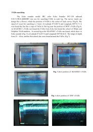
Fig 3 shows the echogram of pelagic and demersal fish school detected by 200 kHz. And 50
kHz. The echogram also showing the vertical distribution curve (VDC) with scale ranging from –80
dB to –30 dB. The VDC detected by 50 kHz Shows the high reverberation level from surface to
bottom. Where as VDC detected by 200 kHz. Showing the less values. The sample of average volume
back scattering strength (SV) and density of fish (N) in each depth layer with integrated for each 0.1
nautical mile of 200 kHz And 50 kHz.
Fig. 4 and Fig. 5 showed the biomass distribution presented by means SV at each 0.1 nautical
mile measured during pre and post-northeast monsoon season, respectively. The SV showing high
value of both season at the shallow water and around the station numbers 25, 26, 27, 36, 41, 42 and 50
where, the stations are between the contour line of 100 m to 200 m. During the survey cruise, the
echogram can be recorded a lot of big pelagic fish school.
The summary of biomass estimation by frequency of 200 kHz. During pre-northeast monsoon
and post-northeast monsoon season are showing in Table 2 and 3. The total estimated biomass during
pre-northeast monsoon season are 1,717,852.38 tons and 956,396.88 tons, respectively. The biomass
distribution are showing in Fig. 6 and 7 for pre and post-northeast monsoon season, respectively.
During the post-northeast monsoon season, the maximum biomass is presented between station
number 50 to 51 with the water depth of 160 m. in the amount of 1,384,550.oo tons. The minimum
biomass is presented between station number 63 to 64 in the amount of 93.06 tons Where the
water depth is 1600 m. The total biomass presented at the water depth of

S2/FR3
108 110 112 114 116 ˚E
8
24
23
22
12
13
11
10
3
4
2
1
39
38
25
26
21
20
14
15
9
8
5
6
40
37
27
19
16
7
54
64
53
55
52
56
41
51
42
50
36
43
35
44
28
34
29
33
18
30
17
31
65
66
63
62
57
58
49
48
45
47
46
32
BINTULU
73
74
72
67
71
68
61
69
60
59
SARAWAK
MIRI
75
70
78
76
77
79
KOTA
KINABARU
SABAH
MUARA
BRUNEI
6
4
2
KUCHING
˚N
Fig. 1 The survey area
ESDU
Fig. 2.
Elementary statistical sampling interval
(ESSR) along the cruise track when the
inter-transect (Dt) equals one elementary
sampling distance unit (ESDU). Tatal
biomass estimation is the summation of
all the abundance of the ESSR area.
Fish School
Fig. 3
The echogram of pelagic and demersal fish schools superimposed with Vertical Distribution
Curve (VDC) detected by 50 kHz. and 200 kHz.
-366-

S2/FR3
Table 2 Summary of biomass estimation by high frequency (200kHz)during premonsoon season off
shore Sarawak, Sabah and Brunei Darussalam. The table show estimation for each station
(ESSR) with cover area is 30x30 nuatical mile
Station Means SV Weight Depth Station Means SV Weight Depth
(dB) (tons) (m) (dB) (tons) (m)
1-2 -72.87 2953.02 46.5 40-41 -90.47 220.47 200.0
2-3 -82.83 424.48 66.2 41-42 -68.77 29489.90 180.6
3-4 -84.37 322.92 71.9 42-43 -68.54 20559.98 119.5
4-5 -76.97 1730.17 70.1 43-44 -76.13 2845.26 95.0
5-6 -74.45 1715.50 38.9 44-45 -83.41 429.57 76.7
6-7 -71.83 2906.67 36.0 45-46 -75.92 1383.76 44.0
7-8 -68.52 5892.31 34.1 46-47 -64.81 10314.61 25.4
8-9 -74.26 2305.88 50.0 47-48 -72.19 4179.90 56.3
9-10 -85.74 260.51 79.5 48-49 -79.40 1314.43 93.2
10-11 -88.88 152.36 95.7 49-50 -72.03 10834.45 140.7
11-12 -68.60 18238.01 107.6 50-51 -51.55 1384550.00 160.9
12-13 -86.25 328.15 112.7 51-52 -86.56 542.54 199.9
13-14 -87.82 204.31 100.6 52-53 -85.01 775.07 200.0
14-15 -82.52 548.99 79.8 53-54 -81.55 1719.86 200.0
15-16 -72.96 3542.96 57.0 54-55 -87.06 484.22 200.0
16-17 -66.01 12012.21 39.0 55-56 -84.98 780.03 200.0
17-18 -71.11 3734.24 39.2 56-57 -93.03 122.22 200.0
18-19 -76.06 1846.91 60.6 57-58 -79.87 2531.68 200.0
19-20 -78.41 1433.26 80.8 58-59 -82.76 1206.11 185.2
20-21 -76.10 3087.13 102.2 59-60 -77.14 4087.36 172.1
21-22 -74.13 6201.32 130.7 60-61 -92.49 138.60 200.0
22-23 -77.60 3106.12 145.4 61-62 -90.41 223.86 200.0
23-24 -77.15 4128.30 174.4 62-63 -81.88 1594.94 200.0
24-25 -82.68 1325.05 200.0 63-64 -94.22 93.06 200.0
25-26 -70.05 18492.92 152.3 64-65 -84.43 886.63 200.0
26-27 -69.11 16483.74 109.4 65-66 -86.44 557.56 200.0
27-28 -67.22 20153.80 86.4 66-67 -78.45 3510.98 200.0
28-29 -76.94 1662.97 66.8 67-68 -90.78 205.45 200.0
29-30 -71.24 4104.37 44.5 68-69 -82.11 1373.12 181.8
30-31 -70.79 2680.09 26.1 69-70 -76.52 2852.94 104.3
31-32 -65.88 9762.12 30.7 70-71 -70.21 23020.09 196.7
32-33 -74.45 1937.49 43.9 71-72 -85.60 677.37 200.0
33-34 -80.59 643.74 60.0 72-73 -81.09 1913.19 200.0
34-35 -80.45 873.43 78.8 73-74 -87.01 489.67 200.0
35-36 -78.06 1882.09 98.0 74-75 -80.63 2126.18 200.0
36-37 -70.29 15615.09 135.7 75-76 -75.11 7235.07 191.0
37-38 -82.76 1300.35 200.0 76-77 -73.94 4985.01 100.5
38-39 -88.99 310.04 200.0 77-78 -80.05 2202.20 181.2
39-40 -80.24 2324.37 200.0 78-79 -74.02 8767.69 180.0
Total = 1717852
-367-

S2/FR3
Table 3. Summary of biomass estimation by high frequency (200 kHz) during post-northeast monsoon
season off shore of Sarawak, Sabah and Brunei Darussalam. The table show estimation
for each station (ESSR) with cover area is 30 x 30 nautical mile.
Station Means SV Weight Depth Station Means SV Weight Depth
(dB) (tons) (m) (dB) (tons) (m)
1-2 -62.73 30475.03 46.5 40-41 -73.28 11544.31 199.9
2-3 -73.22 3901.30 66.6 41-42 -70.87 18149.18 180.5
3-4 -71.76 5959.60 72.8 42-43 -68.17 22378.88 119.4
4-5 -68.99 10906.12 70.3 43-44 -74.53 4107.04 94.9
5-6 -69.81 4966.83 38.6 44-45 -74.11 3672.33 76.9
6-7 -67.90 7283.08 36.5 45-46 -65.60 15003.80 44.3
7-8 -72.96 2165.15 34.7 46-47 -63.93 12804.26 25.7
8-9 -68.89 8018.83 50.5 47-48 -65.69 18732.57 56.4
9-10 -80.16 937.97 79.1 48-49 -75.17 3499.58 93.5
10-11 -77.95 1895.55 96.1 49-50 -68.02 27524.18 142.1
11-12 -65.37 38629.55 108.1 50-51 -69.68 21489.75 162.4
12-13 -74.30 5163.92 113.1 51-52 -69.93 25005.21 200.0
13-14 -76.81 2548.95 99.5 52-53 -76.69 5271.18 200.0
14-15 -72.81 5170.71 80.2 53-54 -68.85 32017.28 200.0
15-16 -74.39 2563.12 57.2 54-55 -80.44 2220.10 200.0
16-17 -62.22 29410.04 39.9 55-56 -82.99 1235.54 200.0
17-18 -68.77 6329.70 38.7 56-57 -75.35 7175.69 200.0
18-19 -69.57 8302.24 61.2 57-58 -71.03 19359.08 200.0
19-20 -75.64 2742.49 81.7 58-59 -71.71 15065.28 181.6
20-21 -74.41 4566.07 102.5 59-60 -66.50 44562.34 162.0
21-22 -74.64 5474.31 129.7 60-61 -82.39 1418.77 200.0
22-23 -67.81 29603.82 145.4 61-62 -71.05 19278.31 200.0
23-24 -76.23 5012.40 171.3 62-63 -78.92 3150.28 200.0
24-25 -72.20 14823.12 199.9 63-64 -83.83 1016.37 200.0
25-26 -68.33 27626.06 152.9 64-65 -89.80 256.87 200.0
26-27 -81.99 850.65 109.5 65-66 -77.60 4274.07 200.0
27-28 -73.48 4784.12 86.8 66-67 -75.46 6992.36 200.0
28-29 -69.23 9861.52 67.2 67-68 -78.56 3421.60 200.0
29-30 -70.61 4755.88 44.5 68-69 -68.36 32650.16 181.9
30-31 -61.99 23392.87 26.1 69-70 -69.69 13898.91 105.4
31-32 -58.10 58311.63 30.7 70-71 -77.63 4185.10 197.5
32-33 -65.59 14907.20 43.9 71-72 -80.30 2295.99 200.0
33-34 -75.17 2253.92 60.2 72-73 -73.85 10120.98 200.0
34-35 -83.11 474.30 78.9 73-74 -78.49 3482.21 200.0
35-36 -78.10 1864.24 97.8 74-75 -85.13 753.75 200.0
36-37 -62.34 95461.97 133.1 75-76 -83.43 1066.63 191.3
37-38 -75.60 6768.21 200.0 76-77 -76.45 2744.86 98.7
38-39 -80.05 2427.10 200.0 77-78 -68.00 35457.60 182.0
39-40 -75.30 7258.02 200.0 78-79 -82.41 1266.92 179.7
Total = 956397
-368-

S2/FR3
108 110 112 114 116 ˚E
8
dB
-50
6
-55
KOTA
KINABARU
-60
MIRI
SABAH
MUARA
BRUNEI
4
-65
-70
-75
-80
BINTULU
SARAWAK
2
-85
-90
-95
KUCHING
˚N
Fig. 4 Distribution of back scattering volume (SV) of fish biomass measured during the pre monsoon
season in Sarawak , Sabah and Brunei Darussalam waters.
108 110 112 114 116 ˚E
8
KOTA
KINABARU
SABAH
MUARA
6
dB
-50
-55
-60
-65
MIRI
BRUNEI
4
-70
-75
BINTULU
SARAWAK
2
-80
-85
-90
KUCHING
˚N
-95
Fig. 5 Distribution of back scattering volume (SV) of fish biomass measured during the post monsoon
season in Sarawak , Sabah and Brunei Darussalam waters.
-369-

S2/FR3
108 110 112 114 116 ˚E
8
dB
1500050
6
1350050
KOTA
KINABARU
SABAH
MUARA
1200050
1050050
900050
MIRI
BRUNEI
4
750050
600050
BINTULU
SARAWAK
2
450050
300050
150050
50
KUCHING
˚N
Fig. 6 Distribution of average fish biomass (ton x 900nm) during the pre monsoon season in
Sarawak , Sabah and Brunei Darussalam waters.
108 110 112 114 116 ˚E
8
tons
100250
6
90250
KOTA
KINABARU
SABAH
MUARA
80250
70250
60250
MIRI
BRUNEI
4
50250
40250
BINTULU
SARAWAK
2
30250
20250
10250
250
KUCHING
˚N
Fig. 7 Distribution of average fish biomass (ton x 900nm) during the post monsoon season in
Sarawak , Sabah and Brunei Darussalam waters.
-370-