5 Four Vectors - Smoot Group Cosmology

Physics 139 Relativity
Relativity Notes 2002
G. F. SMOOT
Oce 398 Le Conte
Department ofPhysics,
University of California, Berkeley, USA 94720
Notes to be found at
http://aether.lbl.gov/www/classes/p139/homework/homework.html
5 Four Vectors
A natural extension of the Minkowski geometrical interpretation of Special Relativity
is the concept of four dimensional vectors. One could also arrive at the concept by
looking at the transformation properties of vectors and noticing they do not transform
as vectors unless another component is added. We dene a four-dimensional vector
(or four-vector for short) as a collection of four components that transforms according
to the Lorentz transformation. The vector magnitude is invariant under the Lorentz
transform.
5.1 Coordinate Transformations in 3+1-D Space
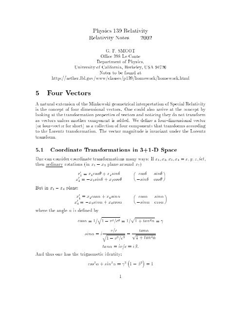
One can consider coordinate transformations manyways: If x 1 ;x 2 ;x 3 ;x 4 =x; y; z; ict,
then ordinary rotations (in x 1 , x 2 plane around x 3 )
x 0 1 = x 1 cos + x 2 sin
cos
sin
x 0 2 = ,x 1 sin + x 2 cos ,sin cos
But in x 1 , x 4 plane:
x 0 1 = x 1 cos + x 4 sin
x 0 4 = ,x 1 sin + x 4 cos
cos
,sin
sin
cos
where the angle is dened by
cos =1=
q
1,v 2 =c 2 =1= p 1+tan 2 =
v=c
sin = i
= q1 , v 2 =c 2
tan
p
1+tan2
tan = iv=c = i:
And thus one has the trignometic identity:
cos 2 + sin 2 = 2 1 , 2 =1
1

x 0 1 = [x 1 +(ict)(i)] = [x 1 , ct]
x 0 4 = [x 4 , ix 1 ]
ict 0 = [ict , ix 1 ]
ct 0 = [ct , x 1 ]
t 0 = [t , x 1 =c]
So the extension to 3+1-D includes Lorentz transformations, if angles are
imaginary.
Really, we are considering the set of all 4 4 orthogonal transformations
matrices in which one angle may be pure imaginary.
In general all angles may be complex, combining real rotations in 2-space with
imaginary rotations relative tot.
An alternate way of writing this is
where = cosh ,1 .
and
x 0 = xcosh , ctsinh
ct 0 = ,xsinh + ctcosh
x 0 = xcos(i)+ictsin(i)
ict 0 = ,xsin(i)+ictcos(i)
= i = icosh ,1 ;
Still another notation is (with x 4 = ict)
The transformation matrix is then
0
B
B
@
x 0 1 = (x 1 + ix 4 )
x 0 4 = (x 4 , ix 1 )
0 0 i
0 1 0 0
0 0 1 0
,i 0 0
Still yet another notation is with x 0 = ct
The transformation matrix is then
x 0 0 = (x 0 , ix 1 )
x 0 1 = (x 1 + ix 0 )
tan = i = iv=c
1
C
C
A
0 1 2 3
0
0 , 0 0
1 , 0 0
B
2@
0 0 1 0
3 0 0 0 1
1
C
A
2

5.1.1 Generalized Lorentz Transformation
For spatial coordinates the Lorentz transform ts the linear form
4X
(x ) 0 = x (1)
=1
subject to the condition that the proper length
(cd ) 2 = ,(ds) 2 = X
(x ) 0 = X
x =(ct) 2 ,j~xj 2 (2)
is an invariant. This condition requires that the coecients
matrix:
X
X
X
=
=
form an orthogonal
=
(3)
where the Kronecker delta is dened by = =
= 1 when = and 0
otherwise.
The invariance group can be enlarged to be the Poincare0 group by the addition
of translations:
(x ) 0 =
4X
=1
x + a (4)
The full group includes: translations, 3-D space rotations, and the Lorentz boosts.
5.2 The Inner Product of 3+1-D Vectors
The denition of the inner product (dot product) must be modied in 3+1 dimensions.
if x 4 = ict. But with our usual convention
~A ~ B = A1 B 1 + A 2 B 2 + A 3 B 3 + A 4 B 4
~A ~ B = A 0 B 0 , A 1 B 1 , A 2 B 2 , A 3 B 3
or with the opposite signature metric one has
~A ~ B = ,A0 B 0 + A 1 B 1 + A 2 B 2 + A 3 B 3
~A ~ B = A 1 B 1 + A 2 B 2 + A 3 B 3 , A 4 B 4
if x 4 = ct which is often the convention for the opposite sign convention. It is an
exercise to show that the inner product is unchanged under a Lorentz transformation.
Can be done simply by substitution. This can be extended to the general class of
Lorentz transformations.
3

5.3 Four Velocity
So we have the position 4-vector ~x =(x 0 ;x 1 ;x 2 ;x 3 ) and the displacement 4-vector
~dx =(dx 0 ;dx 1 ;dx 2 ;dx 3 ). What other 4-vectors are there? That is what other 4-
vectors are natural to construct? What we mean by a four-vector is a four-dimensional
quantity that transforms from one inertial frame to another by the Lorentz transform
which will then leave its length (norm) invariant.
Consider generalizing the 3-vector velocity (v x ;v y ;v z )=(dx=dt; dy=dt; dz=dt)
what can we dotomake this into a 4-vector naturally? One clear problem is that we
are dividing by a component dt of a vector so that the ratio is clearly going to Lorentz
transform in a complicated way. We need to take the derivative with respect to a
quantity that will be the same in all reference frames, e.g. d the dierential of the
proper time, and add a fourth component to make the 4-vector. It is clear that the
derivative of the 4-vector position (ct; x; y; z) with respect to the proper time will
be a 4-vector for Lorentz transformations since (ct; x; y; z) transform properly and d
is an invariant. So we can dene the 4-velocity as
Note that
u = dx
dct
; ~u =
d d ; dx
d ; dy
d ; dz
d
c 2 d 2 = c 2 dt 2 , dx 2 , dy 2 , dz 2 = dt 2
= dt 2 c 2 , v 2 x
, v 2 y
, v 2 z
or the time dilation formula we got before
d
q
dt = 1 , v 2 =c 2 ; and
c 2 , dx
dt
2
!
, dy
dt
= dt 2 c 2 , v 2
dt
d = 1
=
q1 , v 2 =c 2
2
!
, dy 2
dt
So we can now explicitly write out the 4-velocity using the chain derivative rule:
u = dx
d
= dx
dt
~u =(u 0 ;u 1 ;u 2 ;u 3 )=(c;v x ;v y ;v z )=(c; v x ;v y ;v z )
Thus three components of the 4-velocity are the three components of the 3-vector
velocity times .
Note also that the norm - the magnitude or vector invariant length - of the
four-velocity is not only unchanged but it is the same for all physical objects (matter
plus energy). For 3+1 dimensions the norm or magnitude is found from the inner
product or dot product which has the same signature as the metric (see just above)
so that
~u ~u = u 2 0 , u 2 1 , u 2 2 , u 2 3 = 2 c 2 , v 2 x
, v 2 z
, v 2 z
= c 21 , v2 =c 2
1 , v 2 =c = 2 c2
4
dt
d
(5)

Thus every physical thing, including light, moves with a 4-velocity magnitude of c
and the only thing that Lorentz transformations do is change the direction of motion.
A particle at rest is moving down its time axis at speed c. When it is boosted to a
xed velocity, it still travels through space-time at speed c but more slowly down the
time axis as it is also moving in the spatial directions.
One should also note that as the spatial speed (three-velocity) approaches c,
all components of the 4-velocity u are unbounded as !1. One cannot then dene
a Lorentz transformation that moves to the rest frame. Thus all massless particles
will have no rest frame.
5.3.1 Law ofTransformation of a 4-Vector
We can write the transformation in our standard algebraic Lorentz notation
A 0 0 = (A 0 , A 1 ) =1=
q
1, 2
A 0 1 =(A 1,A 0 )
V c
A 0 2 = A 2 ; A 0 3 = A 3
where and refer to the relative velocity V of the frames.
5.3.2 Law ofTransformation of a 4-Velocity
u 0 1 = (u 1 , u 0 )
where and are for the relative velocity of the frames and not of the particle. But
in the formula for the 4-velocity
~u =(u 0 ;u 1 ;u 2 ;u 3 )=(c;v x ;v y ;v z )=(c; v x ;v y ;v z )
The is for the particle! So we should have labeled it p and the and for the
frame transform f and f . Then we have
0 p v0 x= f ( p v x , f p c)
So we can get out a formula for v 0 x
v 0 x
= f p
0 p
(v x , V )=
This is our old friend on the law of transformation of
q
1 , u 2 =c 2 =
q
1,
0 p
q1,p q
1,f
(v x ,V)
q
1 , u 2 =c 2
q
q1 , (u 0 ) 2 =c 2 1 , V 2 =c 2
5
1+u 0 x V=c2

and
which is simply
So
q
1 , (u 0 ) 2 =c 2 =
1
0 p
=
q1 , u 2 =c 2 q
1 , V 2 =c 2
1+u x V=c 2
1
p f (1 , u x V=c 2 )
v 0 x
=
as derived earlier by the dierential route.
Continuing onward
v x , V
1 , u x V=c 2
so that
and
u 0 2 = u 2; or 0 p v0 y = pv y
p
0 p
=
v 0 y
=
v 0 = p
y
0 v y
p
1
f (1 , u x V=c 2 )
q
1 , V 2 =c 2
1 , u x V=c 2 v y
which is the same relationship as before from the dierential Lorentz transform.
Similarly for v 0 z
and v 0 t:
u 0 o = f (u 0 , f u 1 )
Explicitly this is
So
0 c = p f ( p c , p u x V=c)= p f c 1,ux V=c 2
0 p
= p f
1 , ux V=c 2
which is our relation from the transformation of 's and its reciprocal used above.
5.4 Four Momentum
What is the natural extension of the 3-vector momentumto 4-momentum. The answer
is clear from dimensional/transform analysis and from our experimental approach on
how masses transformed. The 4-momentum is simply:
p = m o u ; ~p =(p 0 ;p 1 ;p 2 ;p 3 )=m o (c; v x ;v y ;v z ) (6)
6

The three spatial components are just the Newtonian 3-momentum with the mass of
the particle replaced by m o .
We can see that the 4-momentum also has an invariant norm by making use
of our results for the 4-velocity:
~p ~p p 2 0 , p2 1 , p2 2 , p2 3 = E2 =c 2 , p 2 = m 2 o ~u ~u = m2 o c2
Thus the invariant length of the 4-momentum vector is just the rest mass of the
particle times c.
5.5 The Acceleration Four-Vector
In a similar way one may derive the acceleration four-vector. Again we dierentiate
with respect to the proper time .
a = du
d
The four-vector acceleration will have a part parallel to the acceleration three-vector
and a part parallel to the velocity three-vector.
Exercise: Prove that the inner product of the 4-acceleration and the 4-velocity are
zero; ~a ~u = 0 as they must be if the norm of the four-velocity is to remain constant
c.
We have also constructed the 4-acceleration to be a 4-vector so that ~a ~a is an
invariant. Evaluate it in the rest frame ~a ~a = j~aj 2
~a ~a = j~a rest frame j 2
in any frame. This can be very useful in various calculations and we will use it later
to treat radiation from and accelerating charged particle.
Acceleration 4-vector transforms by the relations:
a 0 0 = f (a 0 , f a 1 ) ; a 0 2 = a 2;
a 0 1 = f (a 1 , f a 0 ) ; a 0 3 = a 3;
This is the best starting place from which to derive the detailed Lorentz
transformation equations for acceleration.
(7)
5.6 The Four Vector Force
We now consider the four-vector force, which we dene the following way:
~F d~p
d
~F d~p
d = d~p dt
dt d = d~p
dt
(8)
7

~F (F 0 ;F 1 ;F 2 ;F 3 )=(W=c; F N 1 ;F N2 ;F N3 )! ~FN ;F ~ N1 ;F N2 ;F N3
(9)
where ~ F N is the three-dimensional Newtonian force, e.g. ~ FN =(F N1 ;F N2 ;F N3 )
Note that the four force can be space-like, time-like and null. If a frame can
be found where the three-force on an object is zero but the object is exchanging
internal energy with the environment, then the four-force is time-like. The converse
is space-like.
Then the 4-vector force ~ F has the same transformation law as all 4-vectors:
~F 0 0 = f
F 0 , f
~ F1
~F 0 1 = f
F 1 , f
~ F0
~F 0 2 = ~ F 2 ; ~ F
0
3 = ~ F 3
So we can now conveniently transform any of the familiar vectors used in mechanics,
but not electric and magnetic elds, and pseudovectors obtained from cross-products,
such as angular momentum and angular velocity. We will treat these later.
The 4-vector force transforms are much easier than the 3-D fource transforms
which involvea 3 . See the homework problem for the transformaiton of acceleration
to grasp how much more complicated it is.
5.7 4-D Potential
It is convenient todophysics in terms of potential and nd the resulting force as the
derivative, e.g. the gradient, of the potential. Classical physics examples are:
F G = ,m r ~ G Newtonian Gravitation
F E = ,q r ~ E Electrostatics (10)
Once we have a 4-D potential, then we need to learn how to take derivatives in 4-D
spaces.
One approach is to make the simplest possible frame-independent (scalar)
estimate of the interaction of two particles. This manner of thinking eventually leads
one to the interaction Lagrangian as a the product of the two currents (electrical,
matter, strong, weak, gravitational).
L = ~ j1 ~ j2 (11)
where is the coupling constant and the next term is the inner (4-D dot) product of
the current of particle 1 and the current of particle 2. When the two currents are in
contact (zero proper distance separation), there is an interaction. When they are not
in proper distance contact, there is no interaction. This means that all interaction
is on the proper distance null (the light cone). Thus there is no action at a proper
distance. It is manifestly invariant as the inner product of two 4-D vectors.
8

From this Lagrangian we can generate the 4-D potential of the eect of all
other currents (or a single current) ~ j2 on our test particle which has current ~ j1 .
~A(~x 1 )=
ZZZZ
f(s 2 12)~ j2 (~x 2 )dV 2 dt 2 =
ZZZZ
f(c 2 (t 1 , t 2 ) 2 , r 2 12)~ jdV dt (12)
where s 2 12 j~x 1 ,~x 2 j 2 =c 2 (t 1 ,t 2 ) 2 ,r12 2 is the invariant separation between ~x 1
and ~x 2 dV is the 3-D spatial volume and dt is the time. f(s 2 12) is a function which is
zero every where but peaks when the square of the 4-vector distance s 2 12
between the
source (2) and the point ofinterest (1) is very small. The integral over f(s 2 12
) is also
normalized to unity. The Dirac delta function is the limiting case for f(s 2 12). Thus
f(s 2 12) is nite only for
s 2 12 = c 2 (t 1 , t 2 ) 2 , r 2 12 2 (13)
Rearranging and taking the square root
c(t 1 , t 2 )
qr12 2 2 r 12
s1 2
r 2 12
r 12 (1
2
2r 2 12
) (14)
So
(t 1 , t 2 ) r 12
c 2
2cr 12
(15)
which says that the only times t 2 that are important in the integral of A ~ are those
which dier from the time t 1 , for which one is calculating the 4-potential, by the
delay r 12 =c ! { with negligible correction as long as r 12 . Thus the Bopp theory
approaches the Maxwell theory as long as one is far away from any particular charge.
By performing the integral over time one can nd the approximate 3-D volume
integral by noting that f(s 2 12) has a nite value only for t 2 =2 2 =2r 12 c, centered
at t 1 , r 12 =c. Assume that f(s 2 12 =0)=K, then
Z Z ~j(t
~A(~x 1 )= ~j(t2 ;~x 2 )f(s 2 12)dV 2 dt 2 K2 , r12 =c; ~x 2 )
dV 2 (16)
c r 12
which is exactly the 3-D version, if we pick K so that K 2 =1.
5.8 Derivative in 4-Space
The 3-D vector gradient operator is DEL:
which behaves as a 3-D vector.
This can be generalized to 4-D:
~r =( @
@x ; @
@y ; @ @z ) (17)
~2 =( @
@x 0
;
@
@x 1
;
9
@
@x 2
;
@
@x 3
) (18)

How does it transform?
~2 0 =( @
@x 0 ;
0
Operate rst on a scalar function (x 0 ;x 1 ;x 2 ;x 3 )
@(x 0 ;x 1 ;x 2 ;x 3 )
@x 0
= X
@ @ @
@x 0 ;
1 @x 0 ;
2 @x 0 ) (19)
3
@
@x
@x
@x 0
where R is the rotation matrix/tensor dened by
= X
@
@x
R (20)
x 0
= X
x = X
a x
(a ,1 ) x 0
(21)
A ,1 = a y ( y means transpose), if a is orthogonal.
x = X
a x 0
(22)
so that
and ~2 is a Lorentz 4-vector.
@ X
@x 0 =
X
x 0
=
~2 0
= X
@
a
@x
a x (23)
a ~2 (24)
5.9 Operate with ~2
Operate with ~2 on a Lorentz 4-vector, to get the dot (inner) product:
~2 ~x = @ct
@ct + @x
@x + @y
@y + @z
@z
= 1+1+1+1=4=invariant (25)
Now operate on velocity 4-vector ~u:
~2 ~u = @c
@ct + @v x
@x
+ @v y
@y
+ @v z
@z
= @ 1
p
@t
+ @ v
1 ,
2 p1
x
@x
+ @ v
,
2 p1
y
@y
+ @ v
,
2 p1
z
@z ,
2
= @ @t ( 1
p )+~ ~v
r( p ) (26)
1 ,
2 1,
2
This equation is an expression related to continuity.
10

5.9.1 Hydrodynamics
Conservation of uid matter is expressed by the equation:
@
@t + ~ r(~v)=0 (27)
If one integrates this equation over a xed volume containing mass M
@
@t
Z
vol
dxdydz +
Z
vol
~r(~v)dxdydz = M (28)
The rst term is the mass contained in the volume and the second part is the
divergence theorem and yields:
@M
@t
Zsurf + ~v ^ndS =0 (29)
ace
@M
@t
= - outward transport of mass and equals the inward transport of mass.
Since our expression for ~2 ~u is
~2 ~u = @ @t ( 1
p )+~ ~v
r( p ) (30)
1 ,
2 1,
2
the role of density isplayed by =1= p 1, 2 .
5.10 The Metric Tensor
Now before moving to make electromagnetism consistent with our relativistic
mechanics, we need to generalize the concepts of the distance, vectors, vector algebra
and tensors as they work in 3+1 D space.
The metric tensor denes the measurement properties of space-time. (Metric
means measure { Greek: metron = a measure.)
Cartesian { at space
(ds) 2 = X i;j
g ij dx i dx j (31)
by denition g ij = g ji since the measure must be symmetric under interchange of
coordinate multiplication order.
In the general case: Cartesian { at space
(ds) 2 = X i;j
g ij dx i dx j = scalar invariant (32)
(Note the superscripts. Section of covariant and contravariant vectors explains this.)
If g ij is diagonal, the coordinates are orthogonal.
11

Physical interpretation: g ii = h 2 i
, where h i is dened by the components of the
vector line element, ds i = h i dx i . An example of this is spherical polar coordinates:
ds 2 = dr 2 + r 2 d 2 + r 2 sin 2 d 2 (33)
2
3
7
6
g ij = 4 1 0 0
0 r 2 0 5 (34)
0 0 r 2 sin 2
For the 3 + 1 dimension Minkowski space-time
ds 2 = d(c) 2 = d(ct) 2 , dx 2 , dy 2 , dz 2 (35)
g =
2
6
4
1 0 0 0
0 ,1 0 0
0 0 ,1 0
0 0 0 ,1
In general the symbol is used to denote the Minkowski metric. Usually it
is displayed in rectangular coordinates (ct; x; y; z) or(x 0 ;x 1 ;x 2 ;x 3 ) but could be
expressed in spherical (ct; r;;) or cylindrical (ct; r;;z) equally well.
The o-diagonal g ij = q h i h j ( ~ ds i ~ ds j ) for i 6= j. An example is skew
coordinates in two dimensions.
3
7
5
(36)
^x 2
O -
^x 1
~dS
^x 2
: - dx2 ~
~S
O:
~dx 1
-
^x 1
By the law of cosines
ds 2 = dx 2 1 + dx 2 2 +2dx 1 dx 2 cos
= g 11 dx 2 1 + g 22dx 2 2 + g 12dx 1 dx 2 + g 21 dx 1 dx 2 (37)
ds 1 = dx 1 ; ds 2 = dx 2
g 11 = h 2 1 =1; g 22 h 2 (38)
2 =1
q
g 12 = g 21 = h 1 h 2 cos = cos (39)
g ij =
1 cos
cos 1
(40)
12

5.11 Contra & Covariant Vectors
First we consider a simple example to illustrate the signicance of contravariant and
covariant vectors. Consider two non-parallel unit vectors ^a 1 and ^a 2 in a plane with
^a 1 ^a 2 = cos 6= 1.
^a 2
^a 2
~S
O - O:
-
^a 1
^a 1
A displacement from O to P can be represented byavector, ~ S. Its components
in the directions of ^a 1 and ^a 2 can be denoted S 1 and S 2 :
~S = S 1^a 1 + S 2^a 2 (41)
^a 2
~S
H O :
S 2
-
^a
1
H -
S 1
Another set of basis vectors ~a 1 and ~a 2 , respectively, may be dened, being
perpendicular to ^a 1 and ^a 2 and having lengths found the following way: Let ^a 3 be a
unit vector normal to the plane, proportional to ^a 1 ^a 2 . Then
~a 1 = ^a 2^a 3
^a 1 ^a 2 ^a 3
=
^e1
sin
(42)
~a 2 = ^a 3^a 1
^a 1 ^a 2 ^a 3
=
^e2
sin
We denote the triple scalar product by [ ] 123
.
(43)
13

6
6
^e 2 O
S > -
SSSSSw
^a 1
^e 1
^a 2
~S
S
:
2
S 1
O
H
-
HHHHHH H ^a HHHHHHHHHHHHH 1
HHY
j~a 2 S 2 j
H
H
H
Hj
H
H
j~a 1 S 1 j
Hj
6
6
^a 2
?
H HHHHH
Hj
The displacement vector, ~ S may also be expressed by its components S 1 and
S 2 as follows:
~S = S 1 ~a 1 + S 2 ~a 2 : (44)
The relations among S 1 , S 2 , S 1 , and S 2 may be found by elementary geometry:
They are:
v 1 = v 1 + v 2 cos (45)
v 1 = v 1 cos + v 2 (46)
Using the original pair of unit vectors,
with the metric tensor
v 1 =(v 1 ,v 2 cos)=sin 2 (47)
v 2 =(,v 1 cos + v 2 )=sin 2 : (48)
S 2 = (S 1 ) 2 +(S 2 ) 2 +2(S 1 )(S 2 )cos
=
2X
i;j=1
Dened to be symmetric.
The tensor g ij is dened by
g ij S i S j (49)
1 cos
g ij =
cos 1
2X
j=1
(50)
g ij g jk = i k : (51)
It is easy to nd that
g ij = 1
sin 2
1 ,cos
,cos 1
: (52)
14

From this relation one nds that
S i = X j
g i;j S j (53)
and
S i = X j
g i;j S j : (54)
The components S i are contravariant and the components S i are covariant.
The square of the length of ~ S is (as given above)
j ~ Sj 2 = X i;j
g ij S i S j =
i;j
X
g ij S i S j ; (55)
but is given more compactly by
S 2 = X j
S j S j (56)
Other relations of interest are:
g ij = Signed Minor of g ij
Det g ij
= Cofactor of g ij
g
(57)
For this example Det g ij = g = sin 2 ; the cofactor of g ij is (,1) i+j g ji =
(,1) i+j g ij because g ij and g ij are symmetric.
Returning to the original sets of basis vectors
and others by cycling indices, by substitution one has:
~a 1 = ^a 2^a 3
^a 1 ^a 2 ^a 3
= ^a 2^a 3
[ ] 123
(58)
^a 1 = ^a2 ^a 3
^a 1 ^a 2 ^a 3 = ^a2 ^a 3
[ ] 123 (59)
Also one has
[ ] 123 = 1
[ ] 123
= 1
sin
Det(g ij )=
(60)
1
Det(g ij ) = 1
sin 2 : (61)
15

5.12 Electric Charge
Wenow consider the implications for electric charge. We dene electric charge density
as the charge per volume, . Wehavealaw of conservation of charge: Charge cannot
be created or destroyed. Thus
So the charge-current density Lorentz 4-vector
(where = 0 ) and
@
@t + ~ r(~v)=0: (62)
~j ~ =(c; v x ;v y ;v z )=(j 0 ;j 1 ;j 2 ;j 3 ) (63)
~2~ j =0 (64)
is the equation for the conservation of charge. ~ j is the 4-vector charge current.
Now consider the vector and scalar potentials of the electromagnetic elds.
ZZZ
~B = r ~ A ~ where A ~
1 ~ jdV
=
c r
~E = , r, ~ 1 @ ~ ZZZ
A
dV
where =
c@t
r
The Lorentz 4-vector potential is
~A =(;A x ;A y ;A z )=(A 0 ;A 1 ;A 2 ;A 3 ) where A = 1 c
Then the inner product gives
ZZZ j dV
r
(65)
(66)
~2 ~ A = 2 A
This is the equation of Lorentz gauge invariance.
5.12.1 Box on ~ Ais a four vector
= @
@ct + @A x
@x + @A y
@y + @A z
@z
= 1 @
c @t + r ~ A=0 ~ (67)
It is clear that ~ j = 0 ~u is a four vector since ~u was constructed to be one and we
constructed ~ j as a scalar (rest frame charge density) times that four vector. However,
I merely asserted that A ~ was a four vector. That is true only if dV=r is invariant
under Lorentz transforms. We have this as an exercise for the student to show
that is true. The following are hints: Show that dV 0 =(1+cos) dV and that
r 0 = r (1 + cos) and thus dV 0 =r 0 = dV=r.
16

5.13 Lorentz Force Law
The 3-D vector form of the force law is
~F=q
~E+~v ~ B
(68)
We need to write this in 4-D vector form to show that it is Lorentz invariant. The
relativistic force lay must involve the particle velocity and the simplest form is linear
in the 4-D velocity. The 4-D vector form then would be
~F = q c
~F ~u; F = q c F u (69)
To obtain the 4-D expression for the electromagnetic elds we need second
rank tensors, i.e. F .
Since wewant the force F to be rest-mass preserving, wehave the requirement
that F u = 0 and thus F u u = 0. Since this must hold for all u , the F must
be antisymmetric.
A cartesian at-space second rank tensor has components C ij . The tensor is
the sum of a symmetric tensor S ij and an antisymmetric tensor A ij :
C ij = 1 2 (C ij + C ji )+ 1 2 (C ij , C ji )
= S ij + A ij (70)
S ij = S ji ; A ij = ,A ji (71)
The property of being symmetric or of being antisymmetric is preserved under
orthogonal transformations.
Now construct the antisymmetric tensor in a generalized curl
F = 2 A , 2 A = @ A , @ A = A ; , A ; (72)
Note that
F 00 = F 11 = F 22 = F 33 =0
F 23 = @A 3
, @A 2
@x 2 @x 3
Similarly, F 31 = B y , F 10 = B z .
=( ~ r ~ A) x =B x
F 10 = @A 0
@x 1
, @A 1
@x 0
= @
@x , @A x
@ct = ,E x
and similarly F 20 = ,E y and F 30 = ,E z . So the full tensor is
F =
2
6
4
0 E x E y E z
,E x 0 ,B z B y
,E y B z 0 ,B x
,E z ,B y B x 0
3
7
5
(73)
17

F is the electromagnetic eld tensor.
The contravariant form of the electromagnetic eld tensor is
F =
2
6
4
0 ,E x ,E y ,E z
E x 0 ,B z B y
E y B z 0 ,B x
E z ,B y B x 0
3
7
5
(74)
One can raise and lower indices by use of the metric tensor.
F = X
In 3-D Maxwell's equations are:
X
g F g (75)
~r B ~ , 1 @ E ~ = ~v c @t c = ~ j
c
~r E ~ =
~r E+ ~ 1 @ B ~
c @t
= 0
~r B ~ = 0 (76)
Now we take the 4-D divergence of the electromagnetic eld tensor
~2 ~ F = ~ j=c (77)
which reduces to the rst two Maxwell equations. The continuity equation is simply
j
=0: (78)
Since there were actually two possible ways to unify the electric and magnetic
elds into a single entity, wenow dene the dual electromagnetic eld tensor:
G =
2
6
4
0 B x B y B z
,B x 0 ,E z E y
,B y E z 0 ,E x
,B z ,E y E x 0
The second set of Maxwell's equations can be simply written as
X
@G
3
7
5
(79)
@x =0 (80)
Or, if one does not wish to resort to the dual electromagnetic eld tensor, then the
second set of Maxwell's equations can be simply written as
a generalized curl.
@ F + @ F + @ F =0 (81)
18

5.14 Transformation of the EM Fields
One can derive the transformation of the electromagnetic eld by using the Lorentz
force law ~ F = q( ~ E + ~ V ~ B) as a denition of the ~ E and ~ B (and by the transformation
of second rank tensors as shown below.) To derive the ~ E and ~ B requires using three
reference frames in order to see how both transform.
Do use the Lorentz force law we need a test electron or charge to probe the
force and thus how the elds must transform. We consider the eld acting on an
electron located at the origin of three reference frames in relative motion.
~F o , E ~ o , B ~ o F ~ , E, ~ B
~
6
6
~ 6 F 0 , E ~ 0 , B ~ 0
S S
0
o S
~V relative toS 0 ~u relative toS o
~v relative toS o
q - - - - -
K
Electron velocity ~v in S
Electron at rest in S Electron velocity ~u in S 0
o
The electron is at rest relative to reference frame S o ,moving with velocity ~v
with respect to reference frame S, and moving with velocity ~u with respect to reference
frame S 0 . We arrange the coordinate systems so that the velocities all lie along the
x axes. Thus the relative velocity V ~ of the frames S and S 0 is given by the velocity
addition formula as
V =
u + v
1+uv=c 2
We can write simple expression for the Lorentz force components in frames S,
S 0 , and S o , respectively:
S S 0 S o
F x = eE x F 0 x = eE0 x
F ox = eE ox
F y = e(E y , vB z ) F 0 y = e(E0 y , uB0 z ) F oy = eE oy
F z = e(E z + vB y ) F 0 z = e(E0 z + uB0 y ) F oz = eE oz
Note that in S o the electron is not moving so that the magnetic eld does not produce
a force.
The equations for the transformation of force (for u 0 x
= 0) give
Then we have
F x = F ox
F 0 x
= q
F ox
F y = F oy
q1 , v 2 =c 2 F 0 = F y oy 1 , u 2 =c
q
2
F y = F oy 1 , v 2 =c 2 F 0 z
= F oz
q1 , u 2 =c 2
E x =Eq
ox
E 0 x
= E ox
E y , vB z = E oy 1 , v 2 =c 2 E 0 y
, uB 0 z
= E oy
q1 , u 2 =c
q
2
E z + vB y = E oz
q1 , v 2 =c 2 E 0 , z uB0 = E y oz 1 , u 2 =c 2
19

We can see at once that E x = E 0 x.From the velocity addition law wehave
and thus
Thus
so that
"
E y ,
v
c =
1
q1 , v 2 =c 2 =
#
u + V
1+uV=c B 2 z
u=c + V=c
1+(u=c)(V=c)
1+ u c
V
c
q q1,u 2 =c 2 1 , V 2 =c 2
E y , vB z
= E oy = q1 E0 , y uB0 z
q
, v 2 =c 2 1 , u 2 =c 2
2
4
3
1+ u V
E
c c
q 5 0 y
, uB 0 z
= q
q1,u 2 =c 2 1 , V 2 =c 2 1 , u 2 =c 2
If these equations are to hold true for all values of u, then since the terms which
contain u must be equal and those that do not must also be equal:
E 0 y =
E y , VB z
q
1,V 2 =c 2
B 0 = ,(V=c)E y + B
q
z
z
1 , V 2 =c 2
Similarly by equating the expression for E oz one nds
E 0 z
=
E z + VB y
q
1,V 2 =c 2
B 0 y
= (V=c)E z + B
q
y
1, V 2 =c 2
This gives the transformation law for 5 of the six components of the
electromagnetic eld. We are missing B x since we started with a stationary electron
in frame S o . This can be found by considering an electron moving at right angles to
B x and recalling that the force is unchanged in the x direction. Thus B 0 x
= B x .
Now do the derivation of eld transformation from the transformation of a
second rank tensor and apply that to F .
F 0
= X
X
a a F (82)
applied to either the electromagnetic eld tensor ~ F or its dual gives
E 0 x
= E x
B 0 x
= B x
E 0 y
= (E y , B z ) B 0 y
= (B y + E z )
E 0 z
= (E z + B y ) B 0 z
= (B z , E y )
(83)
20

5.15 The Equations of Motion for a Charge Particle
The 3-D Lorentz force law
~F = d~p
dt = q( ~ E + ~v c ~ B) (84)
We can turn this into 4-D vector equation by rst replacing dt = d and 3-vector
velocity ~v by the 4-vector velocity ~u.
5.16 The Energy-Momentum Tensor
F = dp
d = qF u (85)
First a brief review to provide motivation for the study and understanding of tensors:
(1) Electromagnetism described by a tensor eld (4 by 4)
(2) Gravity represented by a tensor eld (4 by 4)
(3) elastic phenomena in continuous media mechanics (classical 3 x 3)
(4) metric tensor for generalized coordinates
First we found a 4-vector equation of motion for a single particle:
d~p 2
d = ~ F 2 d~p
d = ~ F
dp
d = F (86)
Next we found the equation of motion for a single particle in an electromagnetic eld
as:
dp
d = m du
0
d = F ~
u (87)
Later we will nd that the equation of motion for a single particle in a weak gravitation
eld is
dp
d = m du
0
d = 1 2 h ;m o u u (88)
The last equation the second rank tensor h is obvious but there is another simple
second rank tensor there m o u u . This is an important tensor. The next paragraph
supplies a little more motivation to study this important and one of the simplest that
one could think to form.
In classical mechanics one has the concept that the integral of the force times
distance is the work done (energy gained) and that the gradient of the potential is
the force.
Z
W =E= ~Fd~x F ~ =, rV ~ (89)
All this points to the need to develop the same concept in 4-D.
E =
Z
~F d~x =
Z d~p
dt d~x = Z d~x
dt d~p = Z
~u d~p (90)
21

From the last part of the equality one nds that the integral to get the \4-potential"
will involve p u . The tensor p u is labeled the energy-momentum tensor. We can
write out explicitly the tensor for a particle.
T = p u = 2m o u u
1 x y z
= m o c 2 2
6
x 2 x
x y x z
4 y x y 2 y
y z
3
7
5
(91)
z x z y z 2 z
since (u )=c(1; x ; y ; z ).
The quantity, 2 m o c 2 = E, seems a bit strange but not so when we consider
a collection of particles or a continuum in density of material, . = 2 o since one
factor of comes from the mass increase and another factor of comes from the
volume contraction due to length contraction along the direction of motion.
2
3
1 x y z
T = c 2
6
x 2 x
x y x z
4
7
y x y 2 (92)
y
y z 5
z x z y z 2 z
and now we see that the energy-momentum tensor components are the transport of
energy-momentum-component in-direction into the -direction.
Consider an interesting case: a large ensemble of non-interacting (elastic
scattering only) particles { an ideal gas. For an ideal gas, < i >= 0 and < i j >=0,
for i 6= j, and ==, so that the energy-momentum tensor is
diagonal
2
3 2
3
c 2 0 0 0 0 0 0
T 0
0
7
y
5 = 0 P
6
4
7 (93)
0 P 5
0 z
0 P
where is the full energy density due to the mass density, and P = 2 which
is easily derived for an ideal gas (PV = nkT = nm).
i
We can write a simple formula for the energy-momentum tensor for a perfect
uid in a general reference frame in which the uid moves with 4-D velocity u as
T =
which reduces to the equation above in its rest frame.
5.17 The Stress Tensor
0 + p=c 2 u u , pg (94)
Now we can consider the case of a medium or eld that can have non-zero o-diagonal
components. First it is good to review the concept of stress. Stress is dened as force
per unit area, (same a pressure which is a particularly simple stress),
22

Imagine a distorted elastic solid or a viscous uid such as molasses in motion.
Imagine a surface (conceptual/mathematical) in the medium (The surface can and
will be curved or distorted.) with a plus and a minus side and unit normal vector for
every point on it. A dierential area element dA, with normal ^n will exert forces on
each of its sides. The forces are equal and opposite by Newton's second law, since
the mass of the element is zero. ~ F total = m~a =0,so ~ F + on, +F , on + =0
The force per unit area on the small element of the surface is the stress. It is
avector, not necessarily known. It underlies the dynamics of continuous media.
Consider a small piece of material at the surface
^n 2
^n 1
6
~F (2) = ~ T (2) dxdz
dz , , dy 1 -
, 3 n3 , dx
~F (3) = T ~ (3) dxdy
~F (1) = ~ T (1) dydz
We dene stress which stretches as positive and stress which compresses as
negative.
Clearly each of the three axes has a vector force associated with it so that we
have a second rank tensor eld associated with the stress. We dene the stress tensor,
E ij T (i)j . Normal Stress is when the vector T (i) is co-directional with the normal
^n (i) .
If E ij = C ij , C is the hydrostatic pressure, if C

z
=
y
6
, , dy
, x
, dx
dz
x+dx
- x
Consider the front face: F x is exerted on it toward inside in the x-direction is
!
F x = ,T xx (x + dx)dxdy = , T xx (x)+ @T xx
@x dx dydz (95)
The force on the back face is
F x =+T xx (x)dxdy = T xx (x)dydz (96)
The net force on the cube is F x is exerted on it toward inside in the x-direction is
F x = , @T xx
dxdydz (97)
@x
If T xx > 0, inside pushes on the outside, pressure: compressive stress. If
T xx < 0, inside pulls on the outside, tension: tensile stress.
T xy and T yx are shear stresses.
z
=
y
6
dy
x
T xy
6
, , , , dz
dx
x+dx
- x
Similarly to the treatment above the net force in the y-direction, F y ,onthe
front and back face is
F y = , @T xy
dxdydz (98)
@x
24

and
Thus the total F x on the material inside is
F x total = , @T xx
@x
F i = ,
F z = , @T xz
dxdydz (99)
@x
3X
i=1
+ @T yx
@x
!
+ @T zx
dxdydz
@x
@T ij
dV (100)
@xi Now consider F y on the two faces perpendicular to x and F x on the two faces
perpendicular to y as exerted from the outside.
F y = ,T xy dA yz
-
F y =+T yx dA yz
?
F y =+T xy dA xz
6
F y = ,T yx dA yz
The sign changes because from the surface the force is toward the inside. Now
calculate the net torque. The two x faces have a counter-clock-wise torque:
torque from x , face = Force moment arm = (T xy dydz)dx=2 (101)
To the net torque is
torque from y , face = ,(T yx dxdz)dy=2 (102)
=(T xy , T yx )dxdydz=2 =I d!
dt
(103)
where I / mr 2 (dxdydz)r 2 is the moment of inertia and d!=dt is the angular
acceleration so that
T xy , T yx / r 2 d!
(104)
dt
as we consider an innitesimal cube, r 2 ! 0 so that
T xy = T yx (105)
which means the stress tensor must be symmetric. The stress tensor is symmetric, so
only six independent components.
25

5.18 Consideration of Shear
Simple shear displacement is like sliding a deck of cards.
-
, ,,
, ,,
A pure shear displacementkeeps the center at the same place and is what our
four forces try to do:
-
6
?
If the little cube is cut dierently, e.g.
dierent eect occurs:
cut at 45 to the previous cube, a
@ @@ ,@
, ,,,
@R ,@ @
, @@@@ @
, ,
, ,,,,,@ , ,
@ , ,
,, @@@@@ ,
@ ,
,
@ , @I
,
@ ,, , ,,,,, @
,
@
,
Thus pure shear is a superposition of tensile and compressive stresses of equal
size at right angles to each other.
Let us follow our example of shear a little further:
T ij =
2
6
4
3
0 T xy 0
7
T xy 0 0 5 (106)
0 0 0
We can look at the transformation properties by considering on the 2 2
portion. Now rotate the axes 45 .How do the tensor components change?
S 0 ij
= X k
X
l
a ik a jl S kl (107)
26

where a ik is the matrix for the coordinate transformation, rotation:
x
0
a11 a
y 0 =
12 x cos sin x
=
a 22 y ,sin cos y
a 21
(108)
For 45 , the rotation matrix is:
so that
[A ij ]=
" 1 p
2 1 p
2
#
, p 1 p 1
2 2
(109)
T 11 = (a 11 ) 2 T 11 + a 12 a 11 T 21 + a 11 a 12 T 12 + a 12 a 21 T 22
= 1 2 (T 11 + T 21 + T 12 + T 22 )=T 21 = T 12 (110)
T 12 = a 11 a 21 T 11 + a 11 a 22 T 12 + a 12 a 21 T 21 + a 12 a 22 T 22
= 1 2 (,T 11 + T 12 , T 21 + T 22 )=0 (111)
T 22 = a 21 a 21 T 11 + a 21 a 22 T 12 + a 22 a 21 T 21 + a 22 a 22 T 22
= 1 2 (T 11 , T 12 , T 21 + T 22 )=,T 21 = ,T 12 (112)
So that for the 45 rotation we have
T 0
ij
=
T21 0
0 ,T 21
(113)
Thus we have shown that a pure shear stress rotated by 45 is equivalent to equal
amounts of tension and compression stress at right angles to each other with the pure
shear bisecting the angle they make.
5.19 Electric and Magnetic Stress
In this section we see that using the Faraday lines of force concept that both the
electric and magnetic eld lines can be under tension or compression and thus by the
argument just above under shear stress.
First consider two opposite charges, magnitude q, a distance 2d apart, located
symmetrically opposite the origin on the x-axis. The force between them is F =
q 2 =(4d 2 ) according to the Coloumblaw. We can imagine putting a metal plate (perfect
conductor) in the y , z plane and know that an image charge will form and have the
same force on it and thus the plate. This makes sense in terms of the Faraday lines
of force. We can calculate the total integrated mean square value of the electric eld
in the y , z plane.
27

y
6
y
6
s
-q
d +q
=
z
s
-
x
H
HHHHHH
s
r
- x
d d
s
Z
The only non-zero component isE x =2qcos=r 2 =2qd=r 3 where r 2 = 2 d 2 .
Z 1
Z
E 2 dA x =4q2 d 2 2d
1
0 ( 2 + d 2 ) 3 =4q2 d 2 d[ 2 + d 2 ]
1
=0 ( 2 + d 2 ) 3 =4q2 d 2 2( 2 + d 2 ) 2 j=0 =1 = 2q2
d 2
(114)
The actual force between the charges is q 2 =(4d 2 ), so that the force per unit
area in eld must be E2
which is a tensile stress and is along the lines of electric eld.
8
Now consider the same situation but with both charges having the same sign.
In this case the lines bend and become tangent to the y , z plane and are clearly in
compression. By symmetry the only non-zero component of the electric eld is that
that goes radially (in the ^ direction).
E 2
= 2q 2q
sin =
2
d d 2 r = 2q
r 3
where E 2 = E2 y +E2 z
. Again we can compute the total integrated mean square electric
eld strength in the y , z plane:
Z
E 2 dA =4q2 Z 1
0
2
r 62d =4q2 Z 1
" #
(r 2 ) , d 2
1
d(r 2 )=4q 2
d 2 (r 2 ) 3 r , d2
2 2(r 2 )
j d2
1 = 2q2
d 2
(115)
Thus again we nd the compressive stress perpendicular to the electric eld lines is
E 2 =8.
Consider another simple case of tension along the lines of electric eld, which
is the familar simple capacitor.
28

+
+
+
+
+
+
+
+
~E
-
-
-
-
-
-
-
-
-
+
+
+
+
+
+
+
+
~E -
-
-
-
-
-
-
-
Clearly the lines of force, electric eld lines are under tension. We can consider
the charge on each of the capacitor faces to have a surface charge density equal to
. Then by Gauss's law we can construct the usual pill box which has a uniform
electric eld passing though the face with area A and not on the sides or outside face.
Thus in Gaussian units 4 = E (in Heavyside-Lorentz units, = E) and the force
between the plates per unit area is
F
A = E
2 = E2
8
(116)
(or in Heavyside-Lorentz units, E 2 =2).
Nowwe turn to magnetic stress. First consider a very long solenoid or a current
sheet.
~F
6 Integral Path
~ j
-
-
~B = 4 ~ c
j`
-
-
?
~F
The magnetic eld is parallel to the solenoid and
Z
~B d ~` = 4 c ~ j
so that B =4j=c`. The Lorentz force on the current is
~F=q(~v ~ B)=~j ~ B
The force per unit area is equal to the average of the magnetic eld at each edge of
the solenoid or for an ideal solenoid this is half the internal magnetic eld. We then
29

have pressure stress
P magnetic = cB2
(117)
8
The factor c depends upon the units one uses. Thus we see that like the electric eld,
the magnetic eld can have compression perpendicular to the magnetic eld lines.
Now we observe tension along magnetic eld lines. Consider two magnets
placed with poles near each other. If the poles are opposite, the magnets are attracted
{ tension in the direction of the lines. If the poles are the same, the magnets are
repulsed { compression perpendicular to the lines.
We can see that this reduces to exactly the same case as for the charges
calculated above by considering two long magnets.
N
S
N
S
N
S
N
S
As the magnets get longer and longer, each pole acts exactly as if it is an
isolated charge and the math is the same.
Now we see that we need to have a momentum-energy tensor or more properly
stress-energy tensor for electromagnetism.
5.20 Stress-Energy Tensor
We need to generalize this to 4-vectors and Lorentz invariance. This will require the
use of second rank tensor - the stress-energy tensor.
In relativistic mechanics for continuous media the energy-momentum or stressenergy
tensor, T , is usually dened as:
T ij = u i u j , E ij ; T i0 = T 0i = u i ; T 00 = (118)
where is the density and E ij is the Cartesian stress tensor usually dened as
the tensor that describes the surface forces on a dierential cube around the point
in question. The normal surface force is pressure but there can be terms for
tension/compression and shearing stress.
Then the equations of motion of a continuous medium is
X
@T
@x
T
;
= f (119)
where f is the 4-force density. That is the net force on material in a volume V is
F =
ZZZ
V
f d 3 V =
ZZ
surf ace
where the last equality comes from invoking Stoke's theorem.
30
T dA (120)

In the case of electromagnetism in the 3-dimensional form the parallel
equations are
~F =
ZZZ
V
ZZZ
~E +~v B ~ d 3 V = E ~ +~j B ~ d 3 V (121)
V
Thus the force density ~ f is
~f = ~ E + ~j ~ B (122)
Now wewant to replace and ~j by the elds via Maxwell's equations.
= ~ r ~ E;
~j = ~ r ~ B , 1 c
Thus
~f =( r ~ E) ~ E+( ~ r ~ B ~ , 1 @ E ~
c @t ~ B
Through suitable use of Maxwell's equations this can be recast to
~f =( ~ r ~ E) ~ E, ~ E( ~ r ~ E)+( ~ r ~ B) ~ B, ~ B( ~ r ~ B) , 1 2 ~ r E 2 + B 2 , 1 c
@ ~ E
@t
@
@t (~ E ~ B)
This is not a particularly elegant expression but is symmetrical in E ~ and B. ~ The
approach can be simplied by introducing the Maxwell Stress Tensor,
T ij =
E i E j , 1
2 ijE 2 +
B i B j , 1
2 ijB 2 (123)
For example the indices i and j can refer to the coordinates x, y, and z, so that the
Maxwell Stress Tensor has a total of nine components (3 3). E.g. with 0 and 0
explicitly stated instead of the units we usually use with c
T ij =
2
6
4
1
2 0
E 2 x , E2 y , E2 z
+
1
2 0
B 2 x , B2 y , B2 z
0 (E x E y )+ 1 0
(B x B y )
1
2 0 Ey,E 2 z,Ex 2 2 +
1
2 0
By,B 2 2 z
,B 2 x
0 (E x E y )+ 1
0
(B x B y )
0 (E x E z )+ 1
0
(B x B z ) 0 (E y E z )+ 1 0
(B y B z )
1
2 0 E
And thus the force per unit volume is then
And by Stoke's Law
~F =
ZZ
surf ace
~f = r ~ ~ T 1 @ S ~ ,
c 2 @t
~ ~ T d ~ A , 1 c 2 d
dt
ZZZ
V
(124)
~Sd 3 V (125)
This turns out to be a much more compact equation in 4-D vector notation.
31

For 4-dimensions the force law isf =F j .
We want the full generalized relation between the energy-momentum tensor,
T , and the 4-force to be:
~F = ~2 ~ T (126)
f = X
@T
@x
X
T
;
T
;
(127)
where the last term represents the repeated indices summation convention. One
uses ;index indicates partial derivative with respect to x rmindex and repeated index to
indicate summation on that index to make the equations easier to write and view.
For example,
f x = T xx;x + T xy;y + T xz;z
force x = pressure + shear stress (128)
For electromagnetism the force equation is
since F ; = j .Thus we have
f = F j = F F ; (129)
T ; = F F ; (130)
A tensor satisfying this equation is
T = , 1 F F
, 1
4
4 F F
T = 1 F F
, 1
4
4 F F
T = , 1 F F
, 1
4
4 g F F
First consider the Maxwell stress tensor,
T ij = 0
E i E j , 1 2 ijE 2
+ 1 0
B i B j , 1 2 ijB 2
T xx = 0
2
E 2 x
, E 2 y
, E 2 z
+ 1
B 2 x
, B 2 y
, B 2 z
2 0
(131)
(132)
(133)
(134)
(135)
T xy = 0 (E x E y )+ 1 0
(B x B y ) (136)
and so on. Bear in mind that the stress tensor is symmetric. It is also possible to
add some additional terms.
T 00 = 1
8
E 2 + B 2 + 1
32
~r( E) ~ (137)
4

T 0i = 1 ~E B ~
4
i + 1 ~r(A 1 E) ~ (138)
4
T i0 = 1 ~E B ~
4
i + 1 ~r( B) ~ ,
@ (E i ) (139)
4
@x 0
The added terms uses the free eld ~j = 0 Maxwell equations and included for
completeness. If the elds are reasonably localized, then T 00 is the eld energy
density, and the T 0i = cP i f ield
is the components of the eld momentum density or
the Poynting vector S.Thus ~ a simplied form is
T = 1
4
2
6
4
T =
" 1
8 (E2 + B 2 )
S ~
~S Maxwell Stress Tensor
#
(140)
E 2 +B 2
2
E y B z , E z B y E z B x , E x B z E x B y , E y B x
E y B z , E z B y
(E 2 x,E 2 y,E 2 z )+(B2 x,B 2 y,B 2 z )
2
E x E y + B x B y E x E z + B x B z
(Ey,E E z B x , E x B z E x E y + B x B 2 x,E 2 2 z )+(B2 y,Bx,B 2 2)
z
y E
2 y E z + B y B z
(E
E x B y , E y B z E x E z + B x B z E y E z + B y B 2 z ,E2 x ,E2 y )+(B2 z ,B2 x ,B2)
y
z
(141)
2
3
7
5
33

5.21 Bopp Theory
In classical electromagnetic theory there are two additional factors that must be taken
into account: (1) the nite speed of light which means that the charge distribution
can change and the change only propagates at the speed of light and (2) the 1/r form
of the potential means that any point charge has innite energy. To take into account
the motion of charges one must end up using retarded potentials. In 3-D one has:
A i (t; ~x 1 )= 1 Z
ji (t,r 12 =c; ~x 2 )
dV 2 (142)
c r 12
Bopp suggested a simpler form of the 4-vector potential which he thought
might handle both problems:
A (~x 1 )=
ZZZZ
j (t 2 ;~x 2 )f(s 2 12)dV 2 dt 2 (143)
Where f(s 2 12) is a function which is zero every where but peaks when the square of
the 4-vector distance s 2 12 between the source (2) and the point ofinterest (1) is very
small. The integral over f(s 2 12) is also normalized to unity. The Dirac delta function
is the limiting case for f(s 2 12). Thus f(s 2 12) is nite only for
Rearranging and taking the square root
s 2 12 = c2 (t 1 , t 2 ) 2 , r 2 12 2 (144)
c(t 1 , t 2 )
qr12 2 2 r 12
s1 2
r 2 12
r 12 (1
2
2r 2 12
) (145)
So
(t 1 , t 2 ) r 12
c 2
2cr 12
(146)
which says that the only times t 2 that are important in the integral of A are those
which dier from the time t 1 , for which one is calculating the 4-potential, by the
delay r 12 =c ! { with negligible correction as long as r 12 . Thus the Bopp theory
approaches the Maxwell theory as long as one is far away from any particular charge.
By performing the integral over time one can nd the approximate 3-D volume
integral by noting that f(s 2 ) has a nite value only for 12 t 2 =2 2 =2r 12 c, centered
at t 1 , r 12 =c. Assume that f(s 2 12
=0)=K, then
A (~x 1 )=
Z
j (t 2 ;~x 2 )f(s 2 12)dV 2 dt 2 K2
c
Z
j (t, r 12 =c; ~x 2 )
r 12
dV 2 (147)
which is exactly the 3-D version shown above ifwe pick K so that K 2 =1.
This manner of thinking eventually leads one to the interaction Lagrangian as
a the product of the two currents (electrical, matter, strong, weak, gravitational).
34

5.22 The Principle of Covariance
The laws of physics are independent of the choice of space-time coordinates.
General Relativity applies this to all conceivable space-time coordinates:
rotating, accelerating, distorting, non-Euclidean, non-orthogonal, etc.
Special Relativity applies this only to the choices of Euclidean (pseudo-
Euclidean), non-rotating coordinate moving with constant velocities with respect to
each other.
Einstein said that this principle is an inescapable axiom, since coordinates are
introduced only by thought and cannot aect the workings of Nature.
Therefore the Principle of Covariance cannot have Physical Content to
determine the laws of any part or eld of physics.
Tensors are essential because all tensor equations of proper form are manifestly
covariant; their functional form does not change when coordinates are changed.
(Proper form means that both sides of the equation result in tensors of the same
rank and, if the equation matches the classical limit formula, then it is the only
correct form. get the stu in these parentheses, precisely right.)
The form of a tensor equation provides no guide for selecting a particular
\xed" or \at rest" coordinate system. However, its content may provide this.
Covariance Language has heuristic invariance:
(1) It guides in proceeding, without telling where to go.
(2) It helps to prevent errors from staying with particular coordinates (through
oversight or error).
(3) One should take as a rst approximation to physical laws those which are simple
in tensor language, but not necessarily simple in a particular coordinate system.
35