WINNER II pdf - Final Report - Cept
WINNER II pdf - Final Report - Cept
WINNER II pdf - Final Report - Cept

Create successful ePaper yourself
Turn your PDF publications into a flip-book with our unique Google optimized e-Paper software.
<strong>WINNER</strong> <strong>II</strong> D1.1.2 V1.2<br />
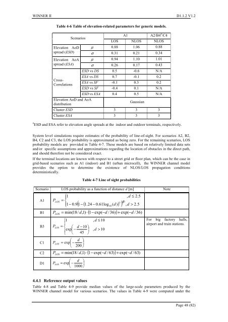
Table 4-6 Table of elevation-related parameters for generic models.<br />
Scenarios<br />
A1 A2/B4 # /C4<br />
LOS NLOS NLOS<br />
Elevation AoD µ 0.88 1.06 0.88<br />
spread (ESD) σ 0.31 0.21 0.34<br />
Elevation AoA µ 0.94 1.10 1.01<br />
spread (ESA) σ 0.26 0.17 0.43<br />
Cross-<br />
Correlations<br />
Elevation AoD and AoA<br />
distribution<br />
ESD vs DS 0.5 -0.6 N/A<br />
ESA vs DS 0.7 -0.1 0.2<br />
ESA vs SF -0.1 0.3 0.2<br />
ESD vs SF -0.4 0.1 N/A<br />
ESD vs ESA 0.4 0.5 N/A<br />
Gaussian<br />
Cluster ESD 3 3 3<br />
Cluster ESA 3 3 3<br />
# ESD and ESA refer to elevation angle spreads at the indoor and outdoor terminals, respectively.<br />
System level simulations require estimates of the probability of line-of-sight. For scenarios A2, B2,<br />
B4, C2 and C3, the LOS probability is approximated as being zero. For the remaining scenarios, LOS<br />
probability models are provided in Table 4-7. These models are based on relatively limited data sets<br />
and/or specific assumptions and approximations regarding the location of obstacles in the direct path,<br />
and should therefore not be considered exact.<br />
If the terminal locations are known with respect to a street grid or floor plan, which can be the case in<br />
grid-based scenarios such as A1 (indoor) and B1 (urban microcell), the <strong>WINNER</strong> channel model<br />
provides the option to determine the existence of NLOS/LOS propagation conditions<br />
deterministically.<br />
Table 4-7 Line of sight probabilities<br />
Scenario LOS probability as a function of distance d [m] Note<br />
A1<br />
P LOS<br />
⎪⎧<br />
1<br />
= ⎨<br />
⎪⎩ 1−<br />
0.9 1<br />
3<br />
( − ( 1.24 − 0.61log ( d)<br />
) )<br />
1 3<br />
10<br />
, d<br />
, d ≤ 2.5<br />
> 2.5<br />
B1 = min( 18/ d,1)<br />
⋅( 1−<br />
exp( −d<br />
/36)) + exp( −d<br />
/36)<br />
B3<br />
C1<br />
P LOS<br />
⎧1<br />
, d ≤10<br />
For big factory halls,<br />
⎪<br />
airport and train stations.<br />
P LOS<br />
= ⎨ ⎛ d −10<br />
⎞<br />
⎪exp⎜<br />
− ⎟ , d > 10<br />
⎩ ⎝ 45 ⎠<br />
P LOS<br />
⎛ d ⎞<br />
= exp⎜<br />
− ⎟<br />
⎝ 200 ⎠<br />
C2 = min( 18/ d,1)<br />
⋅( 1−<br />
exp( −d<br />
/ 63) ) + exp( −d<br />
/ 63)<br />
D1<br />
P LOS<br />
P LOS<br />
⎛ d ⎞<br />
= exp⎜<br />
− ⎟<br />
⎝ 1000 ⎠<br />
4.4.1 Reference output values<br />
Table 4-8 and Table 4-9 provide median values of the large-scale parameters produced by the<br />
<strong>WINNER</strong> channel model for various scenarios. The values in Table 4-9 were computed under the<br />
Page 48 (82)