Final report on link level and system level channel models - Winner

WINNER D5.4 v. 1.4
5.6.1.4 Scenario C1
5.6.1.4.1 LOS propagation conditions
The measured path-loss formula is
where d is the distance.
PL(d) = 41.6 + 23.8 log 10 (d), s = 4 dB (5.60)
The measurement range was limited to 600 m. However, like e.g. in the rural scenario, it is assumed that
the range can be extended to the break-point distance, because the LOS propagation is not very sensitive
to the environment. As well the frequency range can be extended to other frequencies. The path-loss
formula can be expressed as
where d = distance
PL(d) = 41.6 + 23.8 log 10 (d), s = 4.0 dB, 20 m < d d BP
The formula above can be adapted for the frequencies between 2000 and 6000 MHz by replacing the
constant 41.6 by a factor
5.6.1.5 Scenario D1
5.6.1.5.1 LOS model
C(f c ) = 33.2 + 20 log10(f c /(2·10 9 )) (5.62)
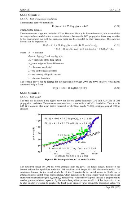
The path loss is shown in the figure below for the two centre-frequencies 2.45 and 5.25 GHz in LOS
propagation conditions. The measurements have been conducted in a 100 MHz bandwidth. The curve for
2.45 GHz contains also a part that is measured in NLOS (or nearly NLOS) conditions around 1000 m
distance.
130
path loss (dB)
120
110
100
90
80
70
PL(d) = -105 + 75.0*log10(d), σ = 2.2 dB
PL(d) = 41.8 + 22.0*log10(d), σ = 2.6 dB
5.25 GHz
Free space
2.45 GHz
PL(d) = 38.3 + 21.1*log10(d), σ = 2.9 dB
100 200 500 1000
distance from MS to BS (m)
Figure 5.88: Rural path-loss at 2.45 and 5.25 GHz.
The measured model for LOS has been extended from the [D5.3] for longer ranges, because it has
become evident that a path-loss model for LOS conditions with longer BS – MS distances is needed. The
maximum distance for the model should be 10 km. Theoretically the model shown in (5.63) can be
extended until so called break-point distance, which depends on the wave-length ? and base station and
mobile station antenna heights h BS and h MS , respectively. After this break-point the loss is proportional to
another, greater path-loss exponent. By flat earth theory this exponent should be 4, but in practice it can
be also smaller or greater. In practice the break point distance varies around the theoretical value. The
Page 128 (167)