Final report on link level and system level channel models - Winner

WINNER D5.4 v. 1.4
IST-2003-507581 WINNER
D5.4 v. 1.4
<strong>Final</strong> Report on Link Level and System Level Channel Models
Date of Delivery to the CEC: Nov. 18 th , 2005
Author(s):
Participant(s):
Workpackage:
Daniel S. Baum, Hassan El-Sallabi, Tommi Jämsä, Juha Meinilä, Pekka
Kyösti, Xiongwen Zhao, Daniela Laselva, Jukka-Pekka Nuutinen, Lassi
Hentilä, Pertti Vainikainen, Jarmo Kivinen, Lasse Vuokko, Per
Zetterberg, Mats Bengtsson, Kai Yu, Niklas Jaldén, Terhi Rautiainen,
Kimmo Kalliola, Marko Milojevic, Christian Schneider, Jan Hansen.
EBIT, EBITT, ETHZ, HUT, KTH, NOK, TUI
WP5 – Channel Modelling
Estimated person months: 66
Security:
Public
Nature:
R
Version: 1.4
Total number of pages: 167
Abstract: This document presents WINNER channel models. The channel models cover WINNER
propagation scenarios for indoor, urban macro-cell and micro-cell, stationary feeder, suburban macro-cell,
and rural macro-cell. Both geometric-based stochastic channel model and reduced-variability (clustered
delay-line) models are presented. The channel models are mainly based on measurement data.
Keyword list: Channel modelling, propagation scenarios, wideband, channel sounder, cluster delay
domain, angle domain, measurements, delay spread, ray, angle-spread, arrival, departure
Disclaimer:
Page 1 (167)

WINNER D5.4 v. 1.4
Executive Summary
This deliverable presents WINNER channel models for link level and system level simulations of short
range and wide area wireless communication systems. The developed channel models follow guidelines
stated in WINNER deliverable D5.2. The models are antenna independent, i.e., different antenna
configurations and different element patterns can be inserted. The covered propagation scenarios are
indoor small office, urban micro-cell, indoor, stationary feeder, suburban macro-cell, urban macro-cell,
and rural macro-cell. The generic WINNER channel model follows a geometric-based stochastic channel
modelling approach, which allows creating of virtually unlimited double directional radio channel model.
Clustered delay line models have also been created for calibration and comparison of different
simulations. The developed models are based on both literature and extensive measurement campaigns
that have been carried out within the WINNER project.
Page 2 (167)

WINNER D5.4 v. 1.4
Authors
Partner Name Phone / Fax / e-mail
ETHZ Daniel S. Baum Phone: +41 44 632 2791
Fax: +41 44 632 1209
E-mail: dsbaum@nari.ee.ethz.ch
HUT Hassan El-Sallabi Phone: +358 9 451 5960
Fax: +358 9 451 2152
E-mail: hsallabi@cc.hut.fi
EBIT Tommi Jämsä Phone: +358 40 344 2000
Fax: +358 8 551 4344
E-mail: tommi.jamsa@elektrobit.com
EBIT Juha Meinilä Phone: +358 40 344 2000
Fax: +358 8 551 4344
E-mail: juha.meinila@elektrobit.com
EBIT Pekka Kyösti Phone: +358 40 344 2000
Fax: +358 8 551 4344
E-mail: pekka.kyosti@elektrobit.com
EBIT Xiongwen Zhao Phone: +358 40 344 2000
Fax: +358 9 5121233
E-mail: xiongwen.zhao@elektrobit.com
EBIT Daniela Laselva Phone: +358 40 344 2000
Fax: +358 8 551 4344
E-mail: daniela.laselva@elektrobit.com
EBIT Jukka-Pekka Nuutinen Phone: +358 40 344 2000
Fax: +358 8 551 4344
E-mail: jukka-pekka.nuutinen@elektrobit.com
Page 3 (167)

WINNER D5.4 v. 1.4
Partner Name Phone / Fax / e-mail
EBIT Lassi Hentilä Phone: +358 40 344 2000
Fax: +358 8 551 4344
E-mail: lassi.hentila@elektrobit.com
HUT Pertti Vainikainen Phone: +358 9 451 2251
Fax: +358 9 451 2152
E-mail: pertti.vainikainen@tkk.fi
HUT Jarmo Kivinen Phone: +358 9 451 2242
Fax: +358 9 451 2152
E-mail: jarmo.kivinen@tkk.fi
HUT Lasse Vuokko Phone: +358 9 451 6064
Fax: +358 9 451 2152
E-mail: lasse.vuokko@tkk.fi
KTH Per Zetterberg Phone: +46 8 7907785
Fax:
E-mail: per.zetterberg@s3.kth.se
KTH Mats Bengtsson Phone: +46 8 7908463
Fax:
E-mail: mats.bengtsson@s3.kth.se
KTH Niklas Jaldén Phone: +46 8 7908415
Fax:
E-mail: niklasj@s3.kth.se
NOK Terhi Rautiainen Phone: +358 50 4837218
Fax: +358 7180 36857
E-mail: terhi.rautiainen@nokia.com
Page 4 (167)

WINNER D5.4 v. 1.4
Partner Name Phone / Fax / e-mail
NOK Kimmo Kalliola Phone: +358 50 4837226
Fax: +358 7180 36857
E-mail: kimmo.kalliola@nokia.com
TUI Marko Milojevic Phone: +49 3677 69 2615
Fax: +49 3677 69 1195
E-mail: marko.milojevic@tu-ilmenau.de
TUI Christian Schneider Phone: +49 3677 69 1157
Fax: +49 3677 69 1113
E-mail: christian.schneider@tu-ilmenau.de
ETHZ Jan Hansen Phone : +41 44 632 0290
Fax: +41 44 632 1209
E-mail: hansen@nari.ee.ethz.ch
Page 5 (167)

WINNER D5.4 v. 1.4
Table of Contents
Part I................................................................................................................. 11
1. Introduction ............................................................................................... 12
2. WINNER Scenarios.................................................................................... 14
2.1 Scenario definitions.............................................................................................................. 14
2.1.1 Scenario A1: Indoor small office .................................................................................. 14
2.1.2 Scenario B1: Urban micro-cell ..................................................................................... 15
2.1.3 Scenario B3: Indoor hotspot ......................................................................................... 15
2.1.4 Scenario B5: Stationary feeder ..................................................................................... 15
2.1.5 Scenario C1: Suburban macro-cell................................................................................ 16
2.1.6 Scenario C2: Urban macro-cell..................................................................................... 16
2.1.7 Scenario D1: Rural macro-cell...................................................................................... 17
3. WINNER Channel Models ......................................................................... 17
3.1 Generic model...................................................................................................................... 17
3.1.1 Large-scale parameters................................................................................................. 17
3.1.2 Average power of ZDSC conditioned on their delays .................................................... 22
3.1.3 Directional distributions of ZDSCs............................................................................... 23
3.1.4 Antenna gain................................................................................................................ 25
3.1.5 Path-loss models.......................................................................................................... 26
3.1.6 Probability of line of sight............................................................................................ 26
3.1.7 Generation of channel coefficients................................................................................ 27
3.2 Reduced variability “clustered delay line” model .................................................................. 29
3.2.1 Scenario A1................................................................................................................. 30
3.2.2 Scenario B1 ................................................................................................................. 31
3.2.3 Scenario B3 ................................................................................................................. 32
3.2.4 Scenario B5 ................................................................................................................. 33
3.2.5 Scenario C1 ................................................................................................................. 37
3.2.6 Scenario C2 ................................................................................................................. 38
3.2.7 Scenario D1................................................................................................................. 39
Part II................................................................................................................ 41
4. Modelling Approaches.............................................................................. 42
4.1 Generic channel modelling approach .................................................................................... 42
4.1.1 Distinction between channel models for link-level and system-level simulation............. 42
4.1.2 Comparison between deterministic and stochastic channel modeling............................. 42
4.1.3 Interference modeling .................................................................................................. 43
4.1.4 Framework .................................................................................................................. 43
4.2 Stationary-feeder scenarios B5 ............................................................................................. 51
4.2.1 B5a LOS stationary feeder: rooftop-to-rooftop.............................................................. 51
4.2.2 B5b LOS stationary feeder: street-level to street-level................................................... 52
4.2.3 B5c hotspot LOS stationary-feeder: below rooftop to street-level.................................. 52
4.2.4 B5d hotspot NLOS stationary feeder: rooftop to street-level.......................................... 52
4.3 Coefficient generation approaches........................................................................................ 53
4.3.1 Stationary stochastic .................................................................................................... 53
Page 6 (167)

WINNER D5.4 v. 1.4
4.3.2 Sum-of-Sinusoids......................................................................................................... 54
4.3.3 Problem details ............................................................................................................ 54
4.3.4 Comparison ................................................................................................................. 55
4.3.5 Kronecker correlation................................................................................................... 55
5. Measurements and Literature Review ..................................................... 56
5.1 Measurement systems .......................................................................................................... 56
5.1.1 Principle of channel sounding....................................................................................... 56
5.1.2 Channel sounders employed ......................................................................................... 56
5.2 Measurement campaigns ...................................................................................................... 61
5.2.1 Scenario A1................................................................................................................. 61
5.2.2 Scenario B1 ................................................................................................................. 62
5.2.3 Scenario B3 ................................................................................................................. 62
5.2.4 Scenario C1 ................................................................................................................. 63
5.2.5 Scenario C2 ................................................................................................................. 63
5.2.6 Scenario D1................................................................................................................. 64
5.2.7 Measurement summary ................................................................................................ 65
5.3 Description of key references ............................................................................................... 67
5.4 Results of analysis items ...................................................................................................... 67
5.4.1 Path-loss and shadow fading ........................................................................................ 67
5.4.2 LOS probability ........................................................................................................... 73
5.4.3 DS and maximum excess-delay distribution.................................................................. 74
5.4.4 Azimuth AS at BS and MS........................................................................................... 79
5.4.5 Distribution of the azimuth angles of the multipath components.................................... 83
5.4.6 Angle proportionality factor ......................................................................................... 85
5.4.7 Modelling of PDP ........................................................................................................ 87
5.4.8 Number of ZDSC......................................................................................................... 91
5.4.9 Distribution of ZDSC delays ........................................................................................ 93
5.4.10 Delay proportionality factor ......................................................................................... 96
5.4.11 Ricean K-factor............................................................................................................ 98
5.4.12 Cross-polarization ratio (XPR) ................................................................................... 101
5.4.13 Large-scale parameter analysis item ........................................................................... 105
5.5 Literature review................................................................................................................ 111
5.5.1 Scenario A1............................................................................................................... 111
5.5.2 Scenario B3 ............................................................................................................... 115
5.5.3 Scenario B5 ............................................................................................................... 116
5.5.4 Scenario C1 ............................................................................................................... 120
5.5.5 Scenario C2 ............................................................................................................... 122
5.5.6 Scenario D1............................................................................................................... 125
5.6 Interpretation of results ...................................................................................................... 127
5.6.1 Path-loss.................................................................................................................... 127
5.6.2 Power-delay profile.................................................................................................... 131
5.6.3 Delay spread.............................................................................................................. 131
5.6.4 K-factor ..................................................................................................................... 132
5.6.5 Cross-polarization discrimination (XPR) .................................................................... 132
5.6.6 Doppler ..................................................................................................................... 132
5.6.7 Angle-spread.............................................................................................................. 132
Page 7 (167)

WINNER D5.4 v. 1.4
5.6.8 Antenna gain.............................................................................................................. 132
5.6.9 Frequency dependence of the propagation parameters................................................. 133
6. Channel Model Implementation ............................................................. 135
6.1 Overview for implementing the model................................................................................ 135
6.1.1 Time sampling and interpolation ................................................................................ 135
6.1.2 Coordinate system...................................................................................................... 135
6.1.3 Generation of correlated large-scale parameters.......................................................... 137
6.2 Interfaces ........................................................................................................................... 138
6.2.1 Example input parameters.......................................................................................... 138
6.2.2 Example output parameters ........................................................................................ 141
6.3 Guidelines and examples on performing system-level simulations....................................... 142
6.3.1 Handover ................................................................................................................... 142
6.3.2 Interference................................................................................................................ 143
6.3.3 Multi-cell and multi-user............................................................................................ 143
6.3.4 Multihop and relaying................................................................................................ 144
7. Test and Verification of the Channel Model and Its Implementation .. 145
7.1 Test cases........................................................................................................................... 145
7.1.1 General test cases....................................................................................................... 145
7.1.2 Input/output parameters.............................................................................................. 145
7.1.3 Validation of computation.......................................................................................... 146
8. References............................................................................................... 148
9. Appendix.................................................................................................. 153
9.1 Other scenarios .................................................................................................................. 153
9.1.1 Scenario definitions.................................................................................................... 153
9.2 Measurement campaigns for other scenarios ....................................................................... 153
9.2.1 Scenario “high mobility short range hot spot”............................................................. 153
9.2.2 Urban ad-hoc peer-to-peer.......................................................................................... 154
9.3 Measurement results for other scenarios ............................................................................. 154
9.3.1 Scenario C2: typical urban macro-cell - KTH campaign.............................................. 154
9.3.2 Scenario “high mobility short range hot spot”............................................................. 156
9.4 Literature review for other scenarios................................................................................... 167
9.4.1 Scenario “high mobility short range hot spot”............................................................. 167
Page 8 (167)

WINNER D5.4 v. 1.4
List of Acronyms and Abbreviations
3GPP
3 rd Generation Partnership Project
3GPP2 3 rd Generation Partnership Project 2
ACF
ADC
AoA
AoD
APP
APS
AS
AWGN
B3G
BER
BRAN
BS
BW
C/I
CDL
CW
D 3 SF
DoA
DoD
DS
EBIT
EBITT
ESPRIT
ETHZ
ETSI
FDD
FIR
FS
GPS
HIPERLAN
HUT
IR
ISIS
KTH
LNS
LOS
MCSSS
METRA
MIMO
MPC
MS
MUSIC
Auto-Correlation Function
Analog-to-Digital Converter
Angle of Arrival
Angle of Departure
A Posteriori Probability
Angle Power Spectrum
Azimuth Spread
Additive White Gaussian Noise
Beyond 3G
Bit Error Rate
Broadband Radio Access Networks
Base Station
Bandwidth
Carrier to Interference ratio
Clustered Delay Line
Continuous Wave
Double-Directional Delay-Spread Function
Direction of Arrival
Direction of Departure
Delay Spread
Elektrobit Ltd
Elektrobit Testing Ltd
Estimation of Signal Parameters via Rotational Invariance Techniques
Eidgenössische Technische Hochschule Zürich (Swiss Federal Institute of Technology
Zurich)
European Telecommunications Standards Institute
Frequency Division Duplex
Finite Impulse Response
Fixed Station
Global Positioning System
High Performance Local Area Network
Helsinki University of Technology (TKK)
Impulse Response
Initialization and Search Improved SAGE
Kungliga Tekniska Högskolan (Royal Institute of Technology in Stockholm)
Log-Normal Shadowing
Line-of-Sight
Multi-Carrier Spread Spectrum Signal
Multi-Element Transmit and Receive Antennas (European IST project)
Multiple-Input Multiple-Output
Multi-Path Component
Mobile Station
Multiple Signal Classification
Page 9 (167)

WINNER D5.4 v. 1.4
NACM
NLOS
NOK
OFDM
OLOS
PAS
PD 3 S
PDP
RMS
PN
RIMAX
RF
RX
SAGE
SCM
SCME
SF
SIMO
SoS
SW
TDL
TUI
TX
WINNER
WPx
XPR
XPR H
XPR V
ZDSC
ZDSC_A
ZDSC_D
No Auto-Correlation Mode
Non Line-of-Sight
Nokia
Orthogonal Frequency-Division Multiplexing
Obstructed Line-of-Sight
Power Azimuth Spectrum
Power Double-Directional Delay-Spectrum
Power-Delay Profile
Root Mean Square
Pseudo Noise
maximum likelihood parameter estimation framework for joint superresolution estimation
of both specular and dense multipath components
Radio Frequency
Receiver
Space-Alternating Generalized Expectation-maximization
Spatial Channel Model
Spatial Channel Model Extended
Shadow Fading
Single-Input Multiple-Output
Sum of Sinusoids
Software
Tapped Delay-Line
Technische Universität Ilmenau
Transmitter
Wireless World Initiative New Radio
Work Package x of WINNER project
Cross-Polarisation Ratio
Horizontal Polarisation XPR
Vertical Polarisation XPR
Zero Delay-Spread Cluster
Zero Delay-Spread Cluster of Arrival
Zero Delay-Spread Cluster of Departure
Page 10 (167)

WINNER D5.4 v. 1.4
PART I
The deliverable D5.4 is divided into two major parts. This first part is the
relatively short main part and contains the essence of the deliverable,
specifically the channel model definition.
Page 11 (167)

WINNER D5.4 v. 1.4
1. Introduction
WINNER project is aiming at a Beyond-3G (B3G) radio system using a frequency bandwidth of 100
MHz for one radio connection and a radio frequency lying most probably somewhere between 2 and 6
GHz in spectrum. The research concerning the suitability of certain communication parameters, like
modulation, coding, symbol rate, MIMO antenna utilisation etc., is performed through extensive
simulations. The simulation results depend strongly on the radio channel. Hence, the radio channel is a
crucial part of the simulation. On one hand, it is very important to use a very accurate and realistic
channel model in the simulation to enable reliable simulation results. On the other hand, the complexity
of the simulation should be kept low. Therefore, the research challenge is to create a channel model which
is realistic enough and simple.
WINNER Work Package 5 (WP5) is focused on multi-dimensional radio channel modelling. Totally six
partners are involved in WP5, namely Elektrobit (EBIT, in year 2004, and Elektrobit Testing EBITT in
year 2005), Helsinki University of Technology (HUT), Nokia (NOK), Royal Institute of Technology in
Stockholm (KTH), Swiss Federal Institute of Technology Zurich (ETHZ), and Technical University of
Ilmenau (TUI). Up to now, the situation is such that there are no widely accepted channel models
available which are suitable for WINNER system parameters. Therefore, WINNER WP5 has to create
new channel models needed in the project. For the initial purposes, WP5 selected and recommended two
existing channel models, which are called initial channel models [D5.1]. The models are 3GPP/3GPP2
Spatial Channel Model (SCM) [3GPP SCM] for outdoor simulations and IEEE 802.11n MIMO model
[802.11n] for indoor simulations. Because the SCM model was not suitable for WINNER simulations as
such, WP5 performed some modifications and implemented the extended SCM model (SCME) [SCME].
However, in spite of these modifications, the initial channel models were not good enough for the
advanced simulations. Consequently new WINNER models are needed.
The WINNER channel models were implemented in two steps. In the first step, channel models for the
most urgently needed propagation scenarios with a limited number of parameters were created.
Propagation scenario means here the propagation environment and certain propagation related parameters
specified to meaningful values. The main difference between different propagation scenarios exists due to
the diverse environments. Channel model parameters were defined for five propagation scenarios
(prioritised scenarios) according to [D7.2], namely indoor small office (A1), urban micro-cell (B1),
stationary feeder (B5), urban macro-cell (C2), and rural macro-cell (D1). These models are described in
the deliverable D5.3 [D5.3]. In the second step the channel models were upgraded so that more
parameters are included in the models. Two more scenarios – indoor (B3) and suburban (C1) – are also
included based on the feedback from other work packages. The channel models created in the first step,
and updated in the second step, are described in this deliverable, D5.4.
In this deliverable, we describe a generic channel model framework that is subsequently used as a basis
for the channel models of all scenarios, except B5. Furthermore, we present clustered delay line (CDL)
models for calibration and comparison simulations. The generic modelling approach allows the creation
of virtually unlimited double directional radio channel realizations. The generic channel model is a raybased
multi-link model that is antenna independent, scalable and capable of modelling channels for
MIMO connections. The models are based on the existing literature and the parameters extracted from
eleven measurement campaigns performed by the WP5. The selection of the model parameters is based
both on the measurements and information found in the literature. The measurements were performed by
five partners, namely EBIT/EBITT, HUT, KTH, NOK, and TUI. Different channel sounders, most of
them capable of measurements at 2 and 5 GHz frequency ranges and 100 MHz bandwidth, were used.
Measurement results were analyzed using beam-forming and super-resolution methods. The analyzed
items, e.g. path loss, shadow fading characteristics, power delay profiles, delay spreads, angle-spreads,
and cross-polarisation ratio (XPR), were analyzed for the scenarios of interest.
In WP5 one activity has been the implementation of the 3GPP/3GPP2 SCM channel model. The model
was implemented in software by the WP5. Later, its extension to 5 GHz frequency range and 100 MHz
bandwidth [SCME] was implemented. The extension work has been published in [BGS+05].
We have compiled a set of requirements from various documents, specifically the WP2 Channel Model
Requirements, the WP5 Deliverable D5.2 [D5.2], WP7 deliverable D7.2 [D7.2], and <strong>report</strong>ed
shortcomings of the channel models selected for initial usage [D5.1]. The main requirements are proper
characterisation of spatial properties for MIMO support, large set of possible channels as well as some
limited randomness channels, consistency in time, frequency and space, e.g. inherent link between angle
spectrum and Doppler spectrum, time-variability of bulk parameters, and extended polarisation support.
The document is organized in a way to provide best readability. Its overall content is divided into 2 major
parts. The first part is relatively short and contains the core information provided in this deliverable. Part I
begins with an introduction, background information concerning our approach, and the requirements on
Page 12 (167)

WINNER D5.4 v. 1.4
the models defined within the WINNER project. It is followed by related scenario definitions. The major
and last chapter of part I contains the brief but comprehensive definition of the channel models. Part II
provides more elaborate background information on model development. It contains detailed discussion
on our modelling approach, the underlying data of our models (measurements and literature review), and
the interpretation thereof. Two more chapters are dedicated to the channel model implementation, and the
test and verification of the model. The document ends with references and further, so far unused results of
this project.
Page 13 (167)

WINNER D5.4 v. 1.4
2. WINNER Scenarios
These are the propagation scenarios defined in WINNER. Scenarios marked in bold are prioritized
scenarios that were modelled and implemented as the WINNER channel models.
Table 2.1: Propagation scenarios defined in WINNER.
Scenario Definition
LOS/N
LOS
Mob. AP ht UE ht Distance
range
Note
A1
In building
Indoor small
office / residential
LOS/
NLOS
0–5
km/h
2 m 1 m 3 - 100 m Deterministic room layout
A2
In building
Indoor to outdoor NLOS 0–5
km/h
AP inside and coverage
outside the building.
B1
Hotspot
Typical urban
micro-cell
LOS/
NLOS
0–70
km/h
Below RT,
e.g. 10 m
1.5 m 20 - 400 m
B2
Hotspot
B3
Hotspot
B4
Hotspot
Bad urban NLOS 0–70
km/h
Indoor LOS 0–5
km/h
Outdoor to indoor NLOS 0–5
km/h
Airport-type. Coverage in
shopping hall with BTS
outside.
B5a
Hotspot
LOS stat. feeder,
rooftop to rooftop
LOS 0 km/h Above RT. Above
RT.
30m - 8 km
B5b
Hotspot
LOS stat. feeder,
street-level to
street-level
LOS 0 km/h 2-5 m 2-5 m
B5c
B5d
LOS stat. feeder,
below-rooftop to
street-level
NLOS stat. feeder,
rooftop to streetlevel
LOS 0 km/h As B1. As B1. As B1. As B1.
NLOS 0km/h As C2. 1.5-10 m. As C2. As C2.
C1
Metropol
Suburban
LOS/
NLOS
0–70
km/h
35 - 3000 m
C2
Metropol
Typical urban
macro-cell
LOS/
NLOS
0–70
km/h
Above RT,
e.g. 32 m
1.5 m 35 - 3000 m
C3
Metropol
C4
Metropol
C5
Metropol
Bad urban NLOS 0–70
km/h
Outdoor to indoor NLOS 0–70
km/h
LOS feeder LOS 0 km/h
D1
Rural
Rural macro-cell
LOS/
NLOS
0–200
km/h
Above RT,
e.g. 45 m
1.5 m 35m - 10 km
D2
Rural
LOS moving
networks (feeder)
LOS 0–300
km/h
2.1 Scenario definitions
In the following subsections, we present WP5 view to the environments of the five prioritized scenarios.
2.1.1 Scenario A1: Indoor small office
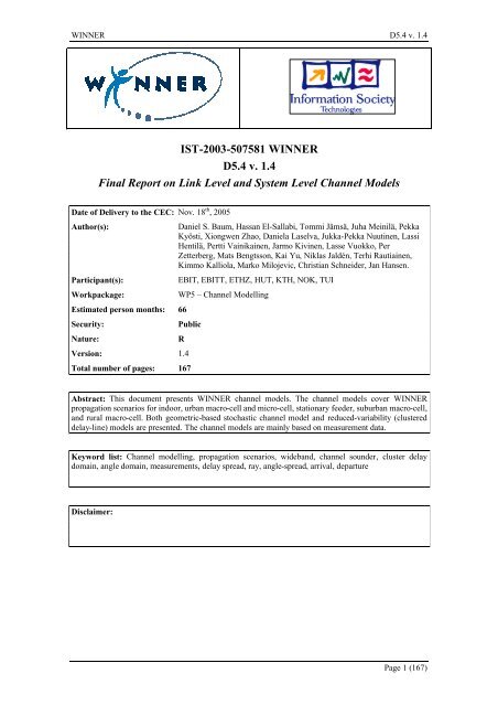
Scenario A1 environment is described in [D7.2]. This represents typical office environment, where the
area per floor is 5000 m 2 , number of floors is 3 and room dimensions are 10 m x 10 m x 3 m and the
corridors have the dimensions 100 m x 5 m x 3 m. The A1 indoor office model is illustrated in Figure 2.1.
Page 14 (167)

WINNER D5.4 v. 1.4
Figure 2.1: Layout of the A1 indoor scenario.
The measured environment resembles this definition, but is not identical [WP5AR]. It is assumed that
propagation parameters can be deduced from these measurements.
2.1.2 Scenario B1: Urban micro-cell
This scenario is defined for environment where both fixed station and mobile station antenna heights are
below surrounding buildings and both are outdoors. This scenario covers both LOS and NLOS
propagation conditions. The environment is defined for Manhattan like grid. The environment streets can
be classified as a main street, where the fixed station is located, perpendicular streets and parallel streets.
The scenario is defined for street distance from 20 m to 400 m. In this environment, the radio propagation
and cell shape are confined within the area defined by the surrounding buildings.
2.1.3 Scenario B3: Indoor hotspot
The scenario B3 is described in [D7.2] and represents a typical indoor hot spot application with a wide
coverage area but non-ubiquitous and low mobility (0-5 km/h). In this scenario traffic of high density can
be expected. Typically application scenarios can be found in conference halls, factory halls, entrance halls
of train stations and airports, where the indoor environment is characterised by large distances. The
dimensions of such large halls can range from 20 m x 20 m x 5 m up to more then 100 m in width and
length as well as 20 m in height. Both LOS and NLOS propagation situations can be found in this
scenario.
2.1.4 Scenario B5: Stationary feeder
The definition of this scenario is less well understood by WP5 than are the others. WP5 found that that
NLOS cases are also of interest for the feeder applications. We therefore discuss models for NLOS cases
as well. The following different feeder scenarios have been studied:
• B5a Hotspot LOS stationary feeder: rooftop-to-rooftop
• B5b Hotspot LOS stationary feeder: street-level-to-street-level.
• B5c Hotspot LOS stationary feeder: blow-rooftop-to-street-level
• B5d Hotspot NLOS stationary feeder: above-rooftop-to-street-level.
The scenarios of B5a and B5b are discussed below:
2.1.4.1 Scenario B5a: LOS stationary feeder: rooftop-to-rooftop
Our understanding of this case is illustrated in Figure 2.2. Wireless feeder master-station, probably on an
elevated building, is connected to one or several wireless feeder peripheral stations. A hot-spot wireless
access point is then connected to the peripheral. As indicated in the picture, a cable is needed to connect
the roof-top wireless feeder peripheral antenna. Alternatively a wireless solution may be possible also for
these hops but then requiring additional antennas and transceivers.
Page 15 (167)

WINNER D5.4 v. 1.4
Feeder-link
Masterstation
Peripheral
Cable
Hot-spot
Figure 2.2: Illustration of LOS stationary feeder: rooftop-to-rooftop.
2.1.4.2 Scenario B5b: LOS stationary feeder: street-level to street-level
Our understanding of this case in indicated in Figure 2.3. Both ends of the link are located a few meters
above ground and the model is aimed for 2-5 meter antenna heights. In many cases it may be possible to
place the antennas high enough such that the first Fresnel zone is clear and therefore free-space
propagation conditions apply.
Hotspot
and feederperipheral.
Feeder-link
Hotspot
and feedermaster.
Figure 2.3: Illustration of wireless LOS feeder-link: street-level.
2.1.5 Scenario C1: Suburban macro-cell
The scenario C1 is defined for a suburban outdoor environment, where the coverage is ubiquitous. In
suburban macrocells base stations are located well above the rooftops to allow wide area coverage.
Buildings are typically low residential detached houses with one or two floors, or blocks of flats with a
few floors. Occasional open areas such as parks or playgrouds between the houses make the environment
rather open. Streets have random orientations, and no urban-like regular strict grid structure is observed.
Vegetation is modest.
2.1.6 Scenario C2: Urban macro-cell
In typical urban macrocell, mobile station is at street level and fixed base station clearly above
surrounding building heights. As for propagation conditions, non- or obstructed line-of-sight is a common
case, since street level is often reached by a single diffraction over the rooftop. The building blocks can
form either a regular Manhattan type of grid, or have more irregular locations. Typical building heights in
urban environments are over four storeys. Outdoor-to-indoor modelling is not part of typical urban
macrocell scenario, but is a different scenario (Table 2.1, C4).
Page 16 (167)

WINNER D5.4 v. 1.4
2.1.7 Scenario D1: Rural macro-cell
Scenario D1 is defined only through its size (100 km 2 ) and hexagonal cell lay-out in [D7.2].
The rural environment we measured is flat, consisting of mainly sparsely located houses along roads that
lead trough fields and some small forests and a small village. This should be considered when interpreting
results based on our model.
3. WINNER Channel Models
This chapter describes WINNER MIMO channel models of seven propagation scenarios for link level and
system level simulations. Link level is defined for a single communication link. System level is defined
for multi communication links and base stations. Five of these scenarios are the prioritized propagation
scenarios defined in the WINNER project in [D7.2] for short range and wide area wireless
communications. The prioritized scenarios are: Scenario A1 for indoor small office environments,
Scenario B1 for microcell urban environment, Scenario B5 for hotspot LOS stationary wireless feeder,
Scenario C2 for Metropolitan ubiquitous coverage in macrocell urban environment, Scenario D1 for
macrocell rural environment. The two additional scenarios are part of the WINNER channel model:
Scenario B3 for indoor propagation and Scenario C1 for macrocell suburban environment.
In this chapter, we provide description of the generic channel model, which is based on the principles of
the SCM [3GPP SCM], for scenario A1, B1, B3, C1, C2, and D1. We also present clustered delay line
(CDL) models for the mentioned six scenarios of interest to generic model, and stationary feeder models
for scenario B5. The generic channel model is a geometric-based stochastic channel model. The following
subsections describe the WINNER phase-I MIMO channel models at 5 GHz.
3.1 Generic model
We apply the framework of the generic channel modelling approach presented in Chapter 4 to WINNER
scenarios A1, B1, B3, C1, C2, and D1. Scenario B5 is not considered in the generic channel model since
it is a stationary wireless feeder scenario, where transmitter and receiver ends are fixed. Scenario B5 is
modelled separately as clustered (tapped) delay line model (CDL) in Section 3.2.4.
The generic channel model generates a number of ZDSCs. Their delays and directional properties are
extracted from statistical distributions that correspond to a specific scenario, which are obtained from
measurement results or from literature. The number of ZDSCs varies from one scenario to another.
Indeed, the number of ZDSCs itself is a random variable. However, in order to reduce the complexity for
simulation purpose, it has been kept as a fixed parameter. The median of the number ZDSCs is selected.
We fix the number of rays within each ZDSC to 10 rays that have same delays and powers and may differ
in angles, either departure or arrival. The directional properties of each ZDSC may vary from one
scenario to another and from departure side to arrival side. The WINNER generic channel model is
antenna independent. Hence, different antenna configurations can be supported. In later terminology, the
downlink is considered, where the transmitter is the fixed station (BS) and the receiver is the mobile
station (MS). However, the same models can also be used for uplink simulations due to the reciprocity of
the radio channel.
3.1.1 Large-scale parameters
The radio channel is in general not stationary. Nevertheless, over short periods of time and space, channel
parameters experience small variations, and the assumption of short-term stationarity is often a very good
approximation. The parameters characterizing our channel model are called bulk parameters. The time
durations, over which these bulk parameters are constant, are termed channel segments a.k.a. drops in the
nomenclature of the SCM. Over time and space, bulk parameters change and we characterize this
variability statistically.
There are a large number of bulk parameters. Bulk parameters include detailed or low-level bulk
parameters such as number of paths, path powers, path angles at both link ends, path elevations at both
link ends, and path delays. To characterize the channel with fewer parameters, higher level, e.g. secondorder,
statistics are extracted on a per-segment basis, which we denote large-scale or dispersion metric
parameters. Large-scale parameters characterize the distributions of and between previously mentioned
low-level bulk parameters. Because realisations of large-scale parameters are drawn only once per
channel segment, they are bulk parameters themselves. The following large-scale parameters are
considered:
• Shadowing. The log-normal shadowing (LNS) value is the common shadowing across (i.e., for
all) clusters. The variability across clusters around the LNS is given by an additive (in logdomain)
Gaussian distribution with a fixed standard deviation of 3 dB.
Page 17 (167)

WINNER D5.4 v. 1.4
• Cross-polarization ratio (XPR). No distinction is made between clusters and segments in the
current model. Therefore, the resulting variability of XPR is equivalent if evaluated across
clusters or across segments.
• Total angle-spread and delay-spread. These parameters characterize the power dispersion in
angle and delay domain across clusters. Note that this is a high-level characterization. The more
detailed properties of angle and delay dispersion are each defined by a set of two variables. This
is firstly, a mean angle and a delay offset for each single cluster, and secondly, an angle-spread
and a delay-spread for each cluster. Here,
• The angle-spread per cluster and delay-spread per cluster values are constants.
• The mean angle per cluster and the delay offset per cluster distributions are functions of
the total (per segment) angle-spread and the total (per segment) delay-spread.
Large-scale parameters of the channel have clear influence on the channel characteristics. This can be
noticed in delay domain characteristics through the RMS delay spread and in the angle domain through
the RMS angle-spread in departure and in arrival. The RMS delay spread has influence on power delay
spectrum and on the probability density function (pdf) of path delays through the parameter r τ .. The
statistical distributions that generate spatial properties of the ZDSCs are functions of RMS angle-spread
through azimuth angle propationality factor ( r ϕ ) and RMS azimuth angle-spread ( σ ϕ ) in the arrival side,
and through departure angle proportionality factor ( r φ ) and RMS departure angle-spread ( σ φ ) in the
departure side. The dispersion parameters σ ϕ and σ φ are sometimes correlated with log-normal
shadowing (LNS), which is important for interference calculations, handover algorithms, etc. For each set
of RMS delay spread and RMS angle-spread departure, RMS angle-spread departure arrival and LNS
within each channel segment, correlation between them has to be considered. These large-scale
parameters are often <strong>report</strong>ed in literature to have log-normal distributions.
Our framework allows for any distribution for the large-scale parameters and also introduces a modelling
of the auto-correlation over the service area. This is achieved by using scenario and parameter specific
g ⋅ to transform the large-scale parameters into a domain where they can be treated as
transformations ( )
Gaussian. The mean, µ , cross-correlation and auto-correlation matrix R ( 0)
are then defined in the
transformed domain. The realizations of the large-scale parameters are then obtained as
−1
0.5
−1
0.5
0.5
5
g R ? x, y + µ
⋅
R 0 is obtained as R ( 0) = EΛ
0.
( ( ) ), where g ( ) is the inverse transform, and ( )
T
from the eigen-decomposition R( 0 ) = EΛE
of R ( 0)
. The auto-correlation is achieved by generating m
( m = 6 for A1, and m = 4 for all other scenarios) independent Gaussian random processes,
? x, y = ξ1 x,
y Kξ
m
x,
y , each one with mean zero and variance one in the positions x, y where the
( ) [ ( ) ( )] T
mobiles are located. The auto-correlation of the process c
( x,
y)
2
E{ ξ ( x y ) ξ ( x , y )} = exp( − r / λ ), where ( ) ( ) 2
c
1, 1 c 2 2
∆
c
∆ r =
no auto-correlation mode (NACM) in which the parameters
the random variable ?( x, y) [ ξ ( x,
y) ( x y)
] T
1
Kξ
m
,
x
1 − x0
+ y1
− y0
m
ξ is given by
. However, we also define a
λ , K ,λ are all set to zero, or equivalently,
= , is randomized independently for each location. The
required parameters for generating the correlated large-scale parameters are thus the transformation
~
s ( x , y)
= g( s( x,
y)
) (or actually its inverse), the mean µ and correlation R ( 0)
of the transformed largescale
parameters, and the de-correlation distance parameters λ , K 1
,λm
.
This information is available in Table 3.1 to Table 3.5. Table 3.1 lists the distribution function for each
modelled parameter in each scenario. For normally distributed random variables the original and
transformed variable is identical, except for the delay-spread in scenario B3, where the transformation is a
9
multiplication with a factor 10 (for numerical reasons). For parameters of log-Gumbel and log-Logistic
distribution, the transformation (and their inverse) are given by:
~
−
s = g s = −Q
1 F log s ,ν ,ς
(3.1)
and
( ) (
Gumbel( 10
( ) ))
−1
( ~ −1
s = g s ) = exp log(10) F Q(
~ s ),ν ,ς
Gumbel
−
1
( ( ))
1 ( F Logistic 10
)
−1
( log(10) F ( Q(
~ s ),ν ,ς ))
−
( s) = −Q
( log ( s)
,ν ,ς )
(3.2)
~
s = g
, (3.3)
−1
s = g ( ~ s ) = exp
Logistic
−
(3.4)
Page 18 (167)

WINNER D5.4 v. 1.4
respectively, where F
Gumbel( x,ν ,ς ) and Logistic ( x,ν,ς )
distributions defined in Section 5.4.3, and Q −1
( x)
variables i.e.
Q
F are the CDF of the Gumbel and Logistic
1
x
∫
−∞
( x) = exp⎜
⎟dt
2π
is the inverse of the CDF for Gaussian random
⎛ − t
⎜
⎝ 2
2
⎞
⎟
⎠
. (3.5)
In Table 3.3, the so-called position ν and scale ς parameters for the distributions are listed, except for
Scenario A1 (with 6 instead of 4 parameters) which is listed in Table 3.5. This means that if the largescale
parameter c is log-Gumbel or log-Logistic, the transformed distribution will have zero mean, and
unit variance, i.e., µ
c
= 0 and R c, c ( 0) = 1.
This can be understood by noting that the mean and variance
are taken into account already in the transformation. For log-normal distributions, we use the
transformation
~
= g( s) = log ( s)
(3.6)
s
10
s
g
=
−1
(
~
~ s
s ) = 10
with the exception of shadow-fading (or sometimes called log-normal shadowing, LNS) where we use
~
= g( s) = 10log ( s)
(3.8)
s
10
s =
−
g
1
(
~ 0.1 s
s ) = 10
~
in order to get the transformed shadow-fading in dB scale. For a log-normal distributed parameter c , the
mean
µ and standard deviation ( 0)
c
R are the mean ν and standard deviation ς listed in Table 3.3.
c,c
For normally distributed bulk parameters no transformation is required (i.e. the transformed and
untransformed value are identical) and thus the mean and
in Table 3.3.
µ and standard deviation ( 0)
c
c,c
(3.7)
(3.9)
R are listed
In Table 3.5, the cross-correlation between the transformed parameters are listed for scenario A1, and in
Table 3.2 for the other scenarios. In teRMS of R ( 0)
, the cross-correlation between parameters r and c is
given by
c r , c
r,
r
r,
c
( 0)
( 0) R ( 0)
R
= . (3.10)
R
Thus by combining the cross-correlation and variance information, the matrix R ( 0)
can be derived. In
Table 3.3, a correlation distance ∆ is listed for each large-scale parameter. The correlation distance is
based on fitting of a single exponential exp( − ∆r / ∆)
to the auto-correlation function of the transformed
large-scale parameter. This value is based on measurements or literature or a combination thereof.
However, since the true auto-correlation actually follows the equation (*) of Section 4.1.4.1.4, i.e.
2
E { ( x , y ) s( x y )} = R( ∆r)
, ( ) ( ) 2
R
s
1 1 2,
2
⎛
⎜
⎝
⎛
⎜
⎝
c,
c
∆ r = x
(3.11)
2 − x1
+ y2
− y1
∆r
⎞ ⎛ ∆r
⎞⎞
⎟
K
⎜ ⎟⎟
(*). (3.12)
λ1
⎠ ⎝ λm
⎠⎠
0.5
0.5,T
( ∆r) = R ( 0) diag⎜exp⎜−
⎟,
,exp⎜−
⎟⎟R
( 0)
. This means
c,
c , will be a mixture of the m exponentials of (*). However,
they are selected in a way that the results are roughly the same as the single exponential. The values of the
“eigenvalue auto-correlation distances” λ
1,
K ,λm
are listed in Table 3.4. Note that there is no one-to-one
mapping between any of the lambda parameters and any of the large-scale parameters. The correlation
distance ∆ is included to allow a more easy interpretation of the auto-regressive characteristics of the
model.
0.5
T 0.5
5
where R ( 0)
is obtained from the eigendecomposition R( 0) = EΛE
as R ( 0) = EΛ
0.
that each autocorrelation function, R ( ∆r)
The justification for the expression (*) is that it produces a model from which it is computationally simple
to generate data, and which at the same time gives a fit to experimental auto-correlation functions which
is typically equally good as the single exponential modelling.
The derivation of some of parameters λ
1,
K ,λm
for each scenario, and in some case also other
parameters, are given in Section 5.4.13 below.
Page 19 (167)

WINNER D5.4 v. 1.4
The values and distributions were obtained from measurements at 5 GHz and from literature.
In simulations which include both LOS and NLOS mobiles, the large-scale parameters of the LOS and
NLOS mobiles are modelled as independent, and thus they should be generated separately.
Delayspread
AoD
spread
AoA
spread
σ
τ
σ
φ
σ
ϕ
Table 3.1: Distribution functions of large-scale parameters.
A1 B1 B3 C1 C2 D1
LOS NLOS LOS NLOS LOS NLOS LOS NLOS NLOS LOS NLOS
LN LN Gumb Gumb N N LN LN LN LN LN
LN LN Logist Gumb N N LN LN LN LN LN
LN LN Logist Gumb N N LN LN LN LN LN
Shadowing LN LN LN LN LN LN LN LN LN LN LN
AoD
Elevation
spread σ
θ
AoA
Elevation
spread σ
ϕ
LN
LN
LN
LN
N
LN
Gumb
Logist
Normal (Gaussian)
Log-normal, i.e., log10(Gauss)
Log-Gumbel
Log-Logistic
Scenarios
Table 3.2: Cross-correlation between large-scale parameters.
B1 B3 C1 C2 D1
LOS NLOS LOS NLOS LOS NLOS NLOS LOS NLOS
σ
φ vs σ
τ 0.50 0.18 0.17 0.13 -0.29 0.3 0.4 -0.07 -0.35
Cross-Correlations
σ
ϕ vs σ
τ 0.76 0.42 -0.2 0.49 0.78 0.7 0.6 0.21 0.12
σ
ϕ vs LNS -0.45 -0.40 -0.17 0.11 -0.16 -0.3 -0.3 -0.11 0.13
σ
φ vs LNS -0.50 0.01 -0.32 -0.18 0.36 -0.4 -0.6 -0.07 0.60
σ
τ vs LNS -0.41 -0.65 0.17 0.34 -0.71 -0.4 -0.4 -0.71 -0.51
σ
φ vs σ
ϕ 0.37 0.07 0.19 0.28 -0.35 0.3 0.4 -0.49 -0.15
Note: Sign of LNS has been defined so that positive LNS means more received power at MS than predicted by PL
model.
Scenarios
Table 3.3: Distributions parameters of large-scale parameters.
B1 B3 C1 C2 D1
LOS NLOS LOS NLOS LOS NLOS LOS LOS NLOS
ν -7.38 -7.09 26 45 -8.8 -7.26 -6.63 -7.8 -7.6
σ τ
ζ 0.24 0.11 8.2 6.9 0.49 0.33 0.32 0.57 0.48
Page 20 (167)

WINNER D5.4 v. 1.4
∆
τ
(m)
6.0 5.0 4.5 1.82 64 40 40 64.2 36.3
ν 0.40 1.24 26.4 38 1.14 0.53 0.93 1.22 0.96
σ φ
ζ 0.23 0.20 10.5 11.7 0.12 0.36 0.22 0.21 0.45
∆
φ 13.2 2.4 2.2 0.62 2.0 30 50 24.8 2.7
σ ϕ
LNS
Notes:
ν 1.4 1.6 13.1 9.5 1.61 1.67 1.72 1.52 1.52
ζ 0.12 0.19 7.6 4.5 0.20 0.3 0.14 0.18 0.27
∆
ϕ
(m)
ζ
(dB)
∆
LNS
(m)
1.6 3.2 0.83 0.61 18.2 30 50 3.5 15.1
2.3 3.1 1.4 2.1
4.0
6.0
8 8
9.1 5.2 4.36 6.16 23.0 50 50 40 120
1. Values for ∆ are merely provided for information. Values of λ (see table below) are used in
coefficient generation.
2. Scenarios C1 LOS and D1 LOS contain two shadowing std. deviations; one (top) for before and
one (bottom) for after the path-loss breakpoint.
Parameters:
ν: Location parameter (i.e., mean in case of normal distribution)
ζ: Scale parameter (i.e., standard deviation in case of normal distribution)
∆: Correlation distance of normal variable
3.5
6.0
8.0
Table 3.4: Lambda parameters.
A1 B1 B3 C1 C2 D1
LOS NLOS LOS NLOS LOS NLOS LOS NLOS NLOS LOS NLOS
λ
1 (m) 2.0 3.5 2.0 5.0 4.5 7.0 40.0 44.0 50.0 3.0 15.0
λ
2 (m) 2.0 2.0 12.0 2.3 0.8 0.6 2.0 30.0 45.0 10.0 2.0
λ
3 (m) 2.0 3.0 3.0 3.0 4.0 1.8 35.0 30.0 40.0 60.0 15.0
λ
4 (m) 3.0 2.5 9.1 5.2 2.2 0.6 27.0 47.0 52.0 42.0 120.0
λ
5 (m) 3.5 5.0
λ
6 (m) 6.0 4.0
Table 3.5: Distribution parameters for A1 sub-scenarios.
Scenario Correlation coefficients Standard
deviations
ς
Means
γ
Decorrelation
distance ∆
(m)
LOS 1,00 0,46 0,74 -0,68 0,49 0,63
0,46 1,00 0,40 -0,05 0,77 0,38
0.27
0.31
-7.40
0.74
7.00
5.90
Page 21 (167)

WINNER D5.4 v. 1.4
0,74 0,40 1,00 -0,44 0,42 0,83
-0,68 -0,05 -0,44 1,00 -0,11 -0,28
0,49 0,77 0,42 -0,11 1,00 0,44
0,63 0,38 0,83 -0,28 0,44 1,00
0.26
3.10
0.20
0.22
1.52
0.00
0.88
0.94
2.30
6.00
1.30
3.50
NLOS 1,00 -0,10 0,31 -0,50 -0,61 -0,05
-0,10 1,00 -0,26 -0,01 0,20 -0,14
0,31 -0,26 1,00 -0,41 -0,28 -0,19
-0,50 -0,01 -0,41 1,00 0,25 0,10
-0,61 0,20 -0,28 0,25 1,00 0,45
-0,05 -0,14 -0,19 0,10 0,45 1,00
0.19
0.23
0.14
3.50
0.21
0.17
-7.60
1.30
1.57
0.00
1.06
1.10
Order of parameters: delay-spread, AoD azimuth-spread, AoA azimuth-spread, shadowing, AoD
elevation-spread, AoA elevation-spread
4.20
4.90
2.50
3.40
3.20
2.60
3.1.2 Average power of ZDSC conditioned on their delays
The average power of every ZDSC is calculated in delay domain as explained in Chapter 4. Two
functions are required to calculate the expected power of each ZDSC conditioned on their delays. They
are the power delay spectrum and the probability density function of ZDSC delays. It is shown in
Chapter 4, that for the case when both P ( τ ) and f ( τ ) are exponential, the expected power of ZDSC
depends on the value of the parameter r τ and the RMS delay spread of the channel segmentσ . In order
to make the average power of ZDSC varying from delay to delay and from one channel segment to
another in a similar manner that is usually seen in measurement results, the shadowing randomization
effect on each ZDSC is modelled. Thus, the expected power of ZDSC of each segment is obtained as:
'
P n
−ζ
2 ⎛
{ }
( rτ
−1) ⎞
10
α τ ∝ exp⎜−τ′
⎟ 10
= E
⎜ rτ
σ ⎟ ⋅ , (3.13)
⎝
τ ⎠
where ζ
n is an i.i.d. Gaussian random variable with zero mean and standard deviation ζ , and the delay
τ ′ is the normalized delay to the delay of the first arrival ZDSC. The normalized delay of the first arrival
ZDSC is zero. For the case when the ZDSC delays have uniform distribution, the expected power of
ZDSC of each segment is obtained as:
'
P n
−ξn
2
10
{ α τ } ∝ exp( −τ
' σ τ
) ⋅10
= E
(3.14)
The ZDSC delay distributions and power delay spectrum of different scenarios are presented in Table 3.6.
For calculation of channels with cross-polarisation, the cross-polarisation ratio (XPR) for vertical to
horizontal (XPR V ) and for horizontal to vertical (XPR H ) are needed (for definition see 5.4.12). The values
XPR V and XPR V of different scenarios are given in Table 3.6.
n
τ
Scenarios
ZDSC
Delay
distribution
Table 3.6: Formulae for calculating the ZDSC power conditioned on delay for the considered
scenarios and XPR V and XPR H .
A1 B1 B3 C1 C2 D1
LOS NLOS LOS NLOS LOS NLOS LOS NLOS NLOS LOS NLOS
Exp Exp Exp Uniform
(0,800ns)
Exp
(0,130ns)
Exp
(0,220ns)
Exp Exp Exp Exp Exp
rτ
3.0 2.4 3.2 2.2 1.90 1.58 2.4 1.5 2.3 3.8 1.7
rτ
−1
rτ
−1
rτ
−1
ϒ
r r r
τ
τ
ζ (dB) 3
τ
'
−t 10
P n ϒ στ
− ξ
n
e 10 n
1
rτ
−1
rτ
−1
rτ
−1
rτ
−1
rτ
−1
rτ
−1
rτ
−1
r r r r r r r
τ
XPR V µ 11.4 9.7 8.6 8 0.5 0.1 7.9 3.3 7.6 6.9 7.9
τ
τ
τ
τ
Page 22 (167)
τ
τ

WINNER D5.4 v. 1.4
(dB)
XPR H
(dB)
σ
µ
σ
3.4 3.5 1.8 1.8 1.07 0.69 3.3 2.5 3.4 2.3 3.5
10.4 10.0 9.5 6.9
3.4 3.1 2.3 2.8
Notes:
Not
avail.
Not
avail.
Not
avail.
Not
avail.
3.7 5.7 2.3 7.2 7.5
2.5 2.9 0.2 2.8 4.0
1. For scenario B3, XPR H values are not available. In the channel model implementation, these
values have been substituted by XPR V .
2. Distribution of XPR is log-normal, i.e., XPR = 10 X/10 , where X is Gaussian with standard
deviation σ and mean µ.
Average powers of the ZDSC are normalized so that the total power of all ZDSCs is equal to one. Then,
the normalized power of the nth ZDSC is
P
'
n
n
= Q
P
∑
n=
1
P
'
n
(3.15)
where Q is the number of ZDSCs. For the case when LOS model is used, the power of the direct
component is considered in the normalization such that the ratio of the direct power to the scattered power
is the K-factor.
'
n
n
=
Q
P
P
( K + 1)∑
n=
1
The K-factor for LOS scenarios can be calculated as given in Table 3.7.
P
'
n
, (3.16)
k
P D
= . (3.17)
k +1
Table 3.7: K factor formulae for LOS scenarios.
Scenarios A1 B1 B3 C1 D1
K [dB] 8.7 + 0.051*d 3+ 0.0142d 6 - 0.26*d 17.1 – 0.021*d 3.7 + 0.019*d
Distance d is in m.
It should be noted that when LOS component exists, the ZDSC will have 10+1 rays.
3.1.3 Directional distributions of ZDSCs
There are two types of angle information for each ZDSC. These are the mean angle and the offset angles
of each ray from the mean within each cluster. The zero mean azimuth departure (azimuth arrival) angle
is the transmitter (receiver) broadside direction. The generated mean angle of departures and angle of
arrivals are relative to the direct path between transmitter and receiver with respect to the broadside of
transmitter or receiver, respectively. The angle definitions and references that are used in the generic
channel model are the same as those presented in [3GPP SCM]. The relation between the mean azimuthdeparture
and the mean azimuth-arrival probability density functions of each ZDSC and their delays is
generated through correlated large-scale parameters used in the corresponding density functions. We
fixed the power azimuth spectrum of each ZDSC at the departure and the arrival sides assuming it as
Laplacian. The RMS angle-spread of each ZDSC is fixed to one value, which may be different in
departure from arrival and may vary from scenario to scenario. However, the power azimuth spectrum
(PAS) and the angle-spread values (AS ) of each ZDSC can be changed in the model if needed. The
distribution parameters of the mean angle of departure (AoD) and the mean angle of arrival (AoA) the
ZDSCs may vary from one scenario to another. The ZDSC azimuth-departure PAS and azimuth-arrival
PAS are defined by 10 rays having predefined offset angles for Laplacian PAS from the mean angles of
Page 23 (167)

WINNER D5.4 v. 1.4
the ZDSC. The 10 rays are spaced in angle domain and have identical power. The power of each ray is
P n /10, where P n is the average power of the nth ZDSC. The offset angle spacing depends on the value of
AS of ZDSC_D for the departure side and value of AS of ZDSC_A for the arrival side. The AS
and
φ
AS are per ZDSC and are different from the
ϕ
φ
ϕ
σ andσ , respectively, which are the composite
angle-spread involving all ZDSC. The rays of the ZDSC have random phases. The angle distributions and
power azimuth spectrum at the transmitter or receiver sides may vary from one scenario to another. Table
3.8 states the angle distributions of different scenarios that are defined in WINNER generic channel
model. The σ and σ influence in generation of the ZDSC directional information through the
φ
ϕ
parameters r
φ andr ϕ , respectively. The location parameter for all distributions is zero and the scaling
parameters are defined by r φ
σ φ for departure angles and by r ϕ
σ ϕ for arrival angles. The generation of
the angle offsets from the rays from cluster mean angle depends on AS
φ for departure side and on
ASϕ
arrival cluster. The offset angles are determined by multiplication of the angles spread per ZDSC
with basis vector of offset angles (BO), e.g., AS
φ *BO. Table 3.9 states the number of ZDSCs and the
number of rays in each cluster as well as their AS
φ and AS
ϕ for the considered scenarios. The angles
of BO vector and the calculation of the offset angles are presented in Table 3.10.
ϕ
φ
Scenarios
AoD
distribution
AoD
scaling
parameter
AoA
distribution
AoA
scaling
parameter
Table 3.8: Distributions of azimuth and departure angles.
A1 B1 B3 C1 C2 D1
LOS NLOS LOS NLOS LOS NLOS LOS NLOS NLOS LOS NLOS
Wrapped Gaussian
2.0σ φ 1.2σ φ 3.4σ φ 1.1σ φ 1.9σ φ 1.3σ φ 1.4σ ϕ 2.3σ φ 3.2σ φ 0.8σ ϕ 1.2σ
φ
Wrapped Gaussian
1.7σ ϕ 2.1σ ϕ 3.6σ ϕ 3.6σ ϕ 1.5σ ϕ 1.6σ ϕ 1.8σ ϕ 1.8σ ϕ 3.2σ ϕ 2.2σ ϕ 1.3σ
ϕ
Scenarios
Table 3.9: Number of ZDSCs and the number of rays in each cluster.
A1 B1 B3 C1 C2 D1
LOS NLOS LOS NLOS LOS NLOS LOS NLOS NLOS LOS NLOS
Number of ZDSC 16 11 8 16 15 24 15 14 20 11 10
Rays per ZDSC 10
AS
φ (deg) 5 5 3 10 4.7 5.5 5 2 2 1.5 1.5
AS
ϕ (deg) 5 5 18 22 5.4 12.5 5 10 15 3 3
Table 3.10: Offset angles Rays within a ZDSC as a function of
AS
φ ,
Ray number Basis vector offset angles (BO) Rays offset angles
1,2 ± 0.0742
3,4 ± 0.2532
5,6 ± 0.4986
7,8 ± 0.8913
AS
ϕ , AS ϕ , and AS θ .
OA = AS X BO
Page 24 (167)

WINNER D5.4 v. 1.4
9,10 ± 1.9718
OA : Offset angles, BO: Basis vector of offset angles
Rays angle offsets of different values of
angle-spread values of
AS
φ or
AS
φ or
AS
ϕ in Table 3.9 can be obtained by multiplying the
AS
ϕ times each angle of the basis vector offset angles (BO). For
example AS
φ = 5; the offset angles of the rays within a ZDSC is OA = 5 x BO = [ ±0.2226 ±0.7596
±1.4960 ±2.6740 ±5.9154].
Elevation angle information are important for indoor environments, i.e., Scenario A1 and B3. The generic
model includes elevation plane for these scenarios. The elevation plane model parameters of these two
scenarios are given in Table 3.11.
Table 3.11: Elevation plane model parameters.
Scenarios
A1
B3
LOS NLOS LOS NLOS
ν (S-dB) 0.88 1.06
σ θ
ζ (S-dB) 0.20 0.21
∆
τ (m) 1.3 3.2
ν (S-dB) 0.94 1.10
σ ϑ
Elevation AoD distribution
ζ (S-dB) 0.22 0.17
∆
τ (m) 3.5 2.6
Wrapped
Gaussian
AoD scaling parameter 1.9 1.4
Elevation AoA distribution
Wrapped
Gaussian
AS θ (deg) 3 3
AS ϕ (deg) 3 3
Cross-Correlations
σ
θ vs σ
τ 0.46 -0.61
σ
ϑ vs σ
τ 0.74 -0.05
σ
θ vs LNS -0.05 0.25
σ
ϑ vs LNS -0.44 0.11
σ
ϑ vs σ
θ 0.44 0.45
3.1.4 Antenna gain
In principle the channel model is antenna independent at both fixed station and mobile station. Any 2D
antenna configuration and pattern can be embedded in the model. If elevation plane parameters are
included, 3D antenna geometries can be embedded. For example, one can use the 3GPP antenna pattern
in WINNER model. The antenna pattern that has been used in [3GPP SCM] at the BS is 3-sector antenna
used for each sector. It is specified by:
A
( γ )
⎡ ⎛ γ ⎞
=−min⎢12
⎜ ⎟
⎢ ⎝γ
3dB
⎣ ⎠
2
, Am
⎤
o
o
⎥, where 180 < φ

WINNER D5.4 v. 1.4
where γ is defined as the angle between the direction of interest and the boresight of the antenna. The
γ
3dB is the 3dB beamwidth in degrees, and A m is the maximum attenuation. For a 3 sector scenario γ
3dB
is 70 degrees, A m = 20dB. However, other antenna patterns can also be used, if needed.
3.1.5 Path-loss models
Path-loss models at 5 GHz for considered scenarios have been developed based on measurement results
or from literature. The developed path models are presented in Table 3.12 including the shadow fading
values. The path-loss models have the form as in (3.21), where d is the distance between transmitter and
receiver, the fitting parameter A includes the path-loss exponent parameter and parameter B is the
intercept.
( d ) B
PL = Alog +
(3.19)
Table 3.12: Path-loss models.
Scenario path loss [dB] shadow
fading
standard
dev.
applicability
range
A1
B1
B3
LOS 18.7 log 10 (d[m]) + 46.8 σ = 3.1 dB 3 m < d < 100 m
NLOS 36.8 log 10 (d[m]) + 38.8 σ = 3.5 dB 3 m < d < 100 m
LOS 22.7 log 10 (d[m])+41.0 σ = 2.3dB 10 m < d < 650 m
NLOS 0.096 d 1 [m] + 65 +
σ = 3.1dB 10 m < d 1 < 550 m
(28 – 0.024d 1 [m]) log 10 (d 2 [m])
w/2 < d 2 < 450 m *)
LOS 13.4 log 10 (d[m]) + 36.9 s = 1.4 dB 5 m < d < 29 m
NLOS 3.2 log 10 (d[m]) + 55.5 s = 2.1 dB 5 m < d < 29 m
C1
s = 4.0 dB
LOS 23.8 log 10 (d) + 41.6
23.8 log 10 (d BP ) ****) +)
40.0 log 10 (d/d BP ) + 41.6 + s = 6.0 dB,
30 m < d < d BP
d BP < d < 5 km
NLOS 40.2 log 10 (d[m]) + 27.7 **) σ = 8 dB 50 m < d < 5 km
C2 NLOS 35.0 log 10 (d[m]) +38.4 ***) σ = 8 dB 50 m < d < 5 km
D1
σ = 3.5dB
LOS 21.5 log 10 (d[m]) + 44.6
21.5 log 10 (d BP ) ****) +)
40.0 log 10 (d/d BP ) + 44.6 + σ = 6.0dB
30 m < d < d BP
d BP < d < 10 km
NLOS 25.1 log 10 (d[m]) + 55.8 σ = 8.0dB 30 m < d < 10 km
*)
w is LOS street width, d 1 is distance along main street, d 2 is distance along perpendicular street.
**) Validity beyond 1 km not confirmed by measurement data.
***)
Validity beyond 2 kms not confirmed by measurement data.
****)
d BP is the break-point distance: d BP = 4 h BS h MS / ?, where h BS is antenna height at BS, h MS is
antenna height at MS, and ? is the wavelength. Validity beyond d BP not confirmed by measurement
data.
+)
BS antenna heights in the measurements: C1 LOS: 11.7 m, D1: 19 – 25 m.
3.1.6 Probability of line of sight
System level simulations require the probability of line of sight for considered scenarios A1, B1, B3, C1,
C2, and D1. They are given as follows:
Page 26 (167)

WINNER D5.4 v. 1.4
3.1.6.1 Scenario A1
3.1.6.2 Scenario B1
⎧
1 d ≤ 2.5m
⎪
P = ⎨
1 − 0.9( 1 − ( 1.24 − 0.61log )
3
) 13
10( d) d > 2.5m
⎪⎩
⎧1 d ≤ 15m
⎪
P = ⎨ 3
1 ( 1 ( 1.56 0.48log ( ))
) 13
⎪ − − −
10
d d > 15m
⎩
(3.20)
(3.21)
where
d = d + d , and d 1 and d 2 are like in Table 2.9.
2 2
1 2
3.1.6.3 Scenario B3
For the big factory halls, airport and train stations:
⎧1,
d < 10m
P LOS
= ⎨
(3.22)
⎩exp(
−(
d −10) / 45)
For big lecture hall or conference hall:
⎪
⎧ 1, d < 5m
P LOS
= ⎨ d − 5
(3.23)
1−
,5 m < d < 40 m
⎪⎩ 150
3.1.6.4 Scenario C1
d[m]
P = exp( − )
(3.24)
500m
3.1.6.5 Scenario C2
For scenario C2, only NLOS is considered. In this case P(LOS) = 0.
3.1.6.6 Scenario D1
3.1.7 Generation of channel coefficients
d[m]
P = exp( − )
(3.25)
1000m
The generation of channel parameters is performed per channel segment. During each channel segment
the AoAs and AoDs, and delays of each ZDSC are fixed while the channel goes through fast fading
according to the virtual motion of the MS, which has a velocity vector v. The assumed system has S
antennas at the transmitter side and U antennas at the receiver side. The WINNER generic channel model
is a geometric-based stochastic model. There are a large number of random variables that are incorporated
in the modelling approach. Hence, many parameters must be fixed within the simulation run to make the
computation time feasible. These parameters may differ from one scenario to another. For instance the
ZDSC angle-spread ( AS or AS ) is fixed for all departure and arrival ZDSCs but may have different
φ
ϕ
angles. These parameters represent some of the characteristics of different scenarios.
To obtain MIMO channel coefficients the following steps are followed:
1) Select one of the scenarios to be simulated: A1, B1, B3, C1, C2, or D1.
2) Assign locations of transmitters (BS), receivers (MS), separating distance and their antenna
orientations. The orientation of MS antenna is drawn from iid uniform distribution U(0 o ,360 o ).
Assign velocity vector to each MS. Assign LOS situation to each location according to the
probability.
3) Calculate the path loss associated with transmitter-receiver of every MS and every BS if needed.
4) Generate the vector ?( x, y)
in the points i
yi
−1
0.5
obtain the large-scale parameters as R ?( x, y)
x , where MSs are located, see Section 6.1.3. Then
( µ )
g +
, the parameters can be found in the
Page 27 (167)

WINNER D5.4 v. 1.4
0.5
Tables of Section Error! Reference source not found.. Note that ( 0)
0.5
5
R ( 0) = EΛ
0.
T
from the eigen-decomposition R( 0 ) = EΛE
of R ( 0)
.
R shall be obtained as
5) Based on the generated large-scale parameters:
a. Generate the delays, azimuth AoD and azimuth AoA of each ZDSC through random
variable generators of the corresponding probability density functions of the selected
scenario. Generate elevation AoD and AoA for indoor Scenarios.
b. Order the delays and normalize them to the smallest delay.
h
c. Calculate the average power of each ZDSC within the channel segment as described in
Section 3.1.2. Assign the power of each ray within the ZDSC as P n
/ M , where M is
the number of rays within ZDSC of a specific scenario, which is fixed to 10 rays.
d. AoA and AoD are sorted in ascending order of absolute values. Shortest delays are are
assosiated to AoA and AoD with smallest absolute values. Respectively, longest delay
is assosiated to AoA and AoD with largest absolute value.
e. Assign angle offset of rays in departure and arrival from predefined set of offset angles
of the selected scenario and assign random phases from U(0 o ,360 o ) to the 10 rays of the
ZDSC. Table 3.10 shows how to obtain offset angles of rays as a function of anglespreads.
f. Randomly couple departure rays to arrival rays.
g. Determine the AoD and AoA for all rays within each ZDSC with respect to the
broadside of transmitter and receiver, respectively.
h. Determine the antenna gain at transmitter G ( AoD ) and receiver ( )
where n is the nth ZDSC and m is the mth ray within the nth cluster.
i. Apply path loss and shadowing to each ray within all ZDSCs.
t
n
G AoA ,
j. With the knowledge of MS velocity vector, fast fading of each ZDSC can be calculated
for every channel segment, while the bulk parameters and MS locations remained fixed.
k. For linear array configuration, the channel coefficient h ( t)
u , s,
n
due to the nth ZDSC
for each antenna pair, element s from transmitter and element u from receiver is given
by:
j⎡
⎣kd
s sin( φm, n ) +Φm,
n⎤
⎦
Gt( φmn
.
) e
⋅
M ⎜
⎟
jkdu
sin( ϕ m,
n)
usn , ,
() =
nσ
SF∑ ⎜
r( ϕmn
,
) ⋅ ⎟ (3.26)
m = 1 ⎜
⎟
jk v cos( ϕ −θ
) t
h t P G e
⎛
⎜
⎝
e
Assuming that cluster n=1 is the one with normalized delay τ 1 =0 (i.e. the cluster with the
lowest delay of all), an optional LOS component may be taken into account as follows:
LOS
u , s,
n
( t)
=
using
where
1
h
K + 1
m,
n
v
⎞
⎟
⎠
[ kd sin( θ ) +Φ ]
j
⎛
s BS LOS
G
⎞
⎜
s(
θBS
) e
⋅
σ
⎟
SFK
j(
kdu
sin( θ MS ) +Φ LOS )
+ δ ( n −1)
⋅ ⎜ Gu
( θMS
e
⋅⎟
(3.27)
K + 1
⎜
jk v cos( θ MS −θ
v ) t
⎟
⎝
e
⎠
u, s,
n
)
⎧1 for n=
0
δ ( n)
= ⎨
⎩ 0 else
φ
n,m is the azimuth angle of departure of mth ray within the nth ZDSC.
ϕ
n,m is the azimuth angle of arrival of mth ray within the nth ZDSC.
M is the number of rays within ZDSC, which is 10.
G ( φ
,m
) is the antenna gain of transmitter (BS) for the mth ray within the nth ZDSC.
t
n
r
n
Page 28 (167)

WINNER D5.4 v. 1.4
G ( ϕ
,m
) is the antenna gain of receiver (MS) for the mth ray within the nth ZDSC.
r
d s
d u
k
n
is the distance between antenna elements of the linear array at transmitter.
is the distance between antenna elements of the linear array at receiver.
is the wave number.
Φ
n,m is the phase of the mth ray within the nth ZDSC.
v
is the speed of the MS.
θ
v
is the angle of the MS velocity vector.
If cross-polarisation is considered, additional cross polarized rays per each ZDSC are generated with
same angle and delay information as those of the co-polarized rays described earlier but different random
xy ,
phases ( Φ ) from uniform distribution U(0°,360°). The complex field pattern at transmitter and
mn ,
receiver for vertical polarisation
receiver
h
F
t
,
h
r
v
F
t
,
v
F
r
respectively, and for horizontal polarisation for transmitter and
vh
F , respectively. The cross-polarized amplitude from vertical to horizontal ( κ
mn , ) or
hv
horizontal to vertical κ
mn , for each ray within each ZDSC are calculated from their corresponding XPR
values given by lognormal distribution of parameters given in Table 3.6 for different scenarios. The κ is
selected for every ray with each cluster from indpenent lognormal distribution with parameters given in
Table 3.3. It is assumed that the XPR random variables of different rays are independent from angles and
delays. The channel coefficient with polarization can be calculated as given in [3GPP SCM] as
h () t = Pσ
usn , ,
n SF
M
∑
m = 1
( φ )
( φ )
( ϕ )
( ϕ )
T
⎛ v
v
⎡
vv vh vh
F ⎤
t m, n ⎡exp( j
mn ,
) κ
m, n
exp( j
,
) ⎤ ⎡F
⎤ ⎞
⎜
Φ
Φ
mn r m,
n
⎢ ⎥ ⎢
⎥ ⎢ ⎥⋅⎟
⎜ h
hv hv hh
h
⎢Ft mn ,
⎥ ⎢κ
mn ,
exp( jΦ m, n) exp( jΦ mn ,
) ⎥ ⎢Fr mn ,
⎥ ⎟
⎜⎣ ⎦ ⎣
⎦ ⎣ ⎦ ⎟
⎜
⎟
⎜
⎟
jkds sin( φmn , ) jkdu sin( ϕm, n ) jk v cos( ϕm,
n−θv
) t
⎜
e e ⋅ e
⎟
⎜
⎟
⎜
⎟
⎝
⎠
(3.28)
For LOS ray (not cluster), the off-diagonal elements of the polarization matrix are zero by definition, i.e.,
the XPR (given by the two κ) is infinity for the LOS ray.
3.2 Reduced variability “clustered delay line” model
This channel model is somehow different from the conventional tapped delay line models in a sense that
fading within each tap is generated by a sum of sinusoids i.e., the rays within the cluster of that tap.
However, it is based on similar principles of the ZDSC channel modelling approach. Clustered delay line
(CDL) model is composed of a number of separate delayed clusters. Each cluster has a number of
multipath components (rays) that have the same known delay values but differ in known angle of
departure and known angle of arrival. The cluster’s angle-spread may be different from that of BS to that
of the MS. The offset angles of the rays depend on the angles spread at BS or MS and are calculated as
shown in Table 3.10. The offset angles represent the Laplacian PAS of each ZDSC. The average power,
mean AoA, mean AoD of clusters, angle-spread at BS and angle-spread at MS of each cluster in the CDL
are extracted or estimated from measurement results at 5 GHz and chip frequency (f c ) of 100 MHz for
Scenarios A1, C2 and D1, and f c =60 MHz for scenario B1 or obtained from literature as in Scenario B5.
In the CDL model each ZDSC is composed of 10 rays with fixed offset angles and identical power. In the
case of ZDSC where a ray of dominant power exists, the ZDSC has 10+1 rays. This dominant ray has a
zero angle offset. The departure and arrival rays are coupled randomly. The CDL table of all scenarios of
interest are give below, where the ZDSC power and the power of each ray are tabulated. The CDL models
offer well-defined radio channels with fixed parameters to obtain comparable simulation results with
relatively non-complicated channel models.
Page 29 (167)

WINNER D5.4 v. 1.4
3.2.1 Scenario A1
The number of different taps in the delay line has been selected according to the measurements data. The
number selected is larger than the median value to represent an environment that is more demanding than
average and also to provide a reasonably low frequency correlation. The offset angles of each ray within
every ZDSC are calculated as shown in Table 3.10. The CDL parameters of LOS and NLOS condition are
given in Table 3.13 and Table 3.14, respectively.
3.2.1.1 LOS
ZDSC
#
delay
[ns]
Table 3.13: Scenario A1: LOS Clustered delay line model, indoor environment.
Power
[dB]
AoD
[º]
AoA
[º]
K-
factor
[dB]
MS speed = 1 m/s,
direction U(0 o ,360 o )
1 0 0 0 0 12.7 -0.23 * -22.9 **
2 5 -1.7 4.25 -61.8 -10.7
3 10 -6.2 0.54 -42.8 -16.2
4 15 -7.7 -4.55 -33.9 -17.7
5 20 -9.3 0.78 -27.2 -19.3
6 25 -12.1 -3.14 16.6 -22.1
7 30 -12.7 3.74 41.2 -22.7
8 35 -12.7 -2.83 -15.6 -22.7
9 45 -14.7 2.01 2.54 -24.7
10 55 -16.3 5.83 -89.1 -26.3
11 65 -16.8 -10.9 40.9 -26.8
-∞
Number of rays /ZDSC = 10 +
Ray Power [dB]
ZDSC AS at MS [º] = 5
ZDSC AS at BS [º] = 5
Composite AS at MS [º] = 32.5
Composite AS at BS [º] = 5.1
12 75 -18.4 -13.4 124.0
-28.4
*
**
+
Power of dominant ray,
Power of each other ray
Clusters with high K-factor will have 11 rays.
3.2.1.2 NLOS
ZDSC #
Table 3.14: Scenario A1: NLOS Clustered delay line model, indoor environment.
delay
[ns]
Power
[dB]
AoD
[º]
AoA
[º]
K-
factor
[dB]
MS speed = 1 m/s,
direction U(0 o ,360 o )
1 0 0 0 0 0
2 5 -0.9 17.1 19.4 -10.9
3 10 -1.5 -2.09 33.2 -11.5
4 15 -1.6 4.99 15.2 -11.6
5 20 -2.0 -11.4 -20.7 -12.0
6 25 -2.6 -22.9 71.2 -12.6
7 30 -3.4 43.4 48.3 -13.4
8 35 -4.5 -32.2 92.6 -14.5
9 40 -5.5 -22.0 49.0 -15.5
10 45 -5.5 52.4 43.4 -15.5
11 50 -5.0 1.57 -66.1 -15.0
-∞
Number of rays /ZDSC = 10
Ray Power [dB]
ZDSC AS at MS [º] = 5
ZDSC AS at BS [º] = 5
Composite AS at MS [º] = 39.1
Composite AS at BS [º] = 23.2
12 55 -4.7 37.8 -30.8
-14.7
Page 30 (167)

WINNER D5.4 v. 1.4
13 65 -5.4 8.39 -59.0 -15.4
14 75 -9.0 -27.5 14.1 -19.0
15 85 -11.3 -43.9 -7.76 -21.3
16 95 -12.5 13.7 -0.59 -22.5
17 105 -13.6 63.8 -13.4 -23.6
18 115 -15.1 2.31 3.29 -25.1
19 125 -16.8 8.77 4.22 -26.8
20 135 -18.7 31.1 15.9 -28.7
3.2.2 Scenario B1
The parameters of the CDL model have been extracted from measurements with chip frequency of 60
MHz at frequency range of 5.3 GHz. The number of ZDSCs is selected to be close to the median and
provide low frequency correlation. The CDL parameters of LOS and NLOS condition are given in Table
3.15 and Table 3.16, respectively.
3.2.2.1 LOS
Table 3.15: Scenario B1: LOS Clustered delay line model.
ZDSC #
delay
[ns]
Power
[dB]
AoD
[º]
AoA
[º]
K-
factor
[dB]
MS speed = 50 km/h,
direction U(0 o ,360 o )
1 0 0 0 0 16 -0.11 * -26.11 **
2 10 -1.2 -22 -10 9 -1.72 -20.7
3 25 -7.4 -12 20 3 -9.16 -22.16
4 30 -7.4 -12 20 -17.4
5 45 -8.4 -2 -123 -18.4
6 65 -13.0 10 -31 -23
7 85 -15.1 -4 161 -25.1
8 105 -16.1 8 -7
-26.1
-∞
Number of rays
/ZDSC =10 +
Ray Power [dB]
ZDSC AS at MS [º] = =18
ZDSC AS at BS [º] =3
Composite AS at MS [º]
=37.1
Composite AS at BS [º] =
5.6
*
**
+
Power of dominant ray,
Power of each other ray
Clusters with high K-factor will have 11 rays.
3.2.2.2 NLOS
ZDSC
#
delay
[ns]
Power
[dB]
Table 3.16: Scenario B1: NLOS Clustered delay line model.
AoD
[º]
AoA
[º]
K-
factor
[dB]
MS speed = 50 km/h,
direction U(0 o ,360 o )
1 0 -1.25 4 0 9 -1.8 * -20.8 **
2 10 0 40 25 6 -1 * -17 *
3 40 -0.38 -10. 29 -10.38
4 60 -0.10 48. -31 -10.10
5 85 -0.73 -36. 37 -10.73
6 110 -0.63 -40 21 -10.63
7 135 -1.78 -26 13
-∞
Number of rays /ZDSC
= 10 +
Ray Power [dB]
-11.78
ZDSC AS at MS [º]
=22
ZDSC AS at BS [º]
=10
Composite AS at MS
[º] =36.4
Composite AS at BS
[º] =12.4
Page 31 (167)

WINNER D5.4 v. 1.4
8 165 -4.07 -28 117 -14.07
9 190 -5.12 -12 21 -15.12
10 220 -6.34 -14 1 -16.34
11 245 -7.35 14 15 -17.35
12 270 -8.86 8 9 -18.86
13 300 -10.1 -24 19 -20.1
14 325 -10.5 -14 1 -20.5
15 350 -11.3 -22 -13 -21.3
16 375 -12.6 2 11 -22.6
17 405 -13.9 8 -1 -23.9
18 430 -14.1 -2 43 -24.1
19 460 -15.3 -10 33 -25.3
20 485 -16.3 -54 -19 -26.3
*
**
+
Power of dominant ray,
Power of each other ray
Clusters with high K-factor will have 11 rays.
3.2.3 Scenario B3
3.2.3.1 LOS
ZDSC
#
Delay
[ns]
Power
[dB]
Table 3.17: Scenario B3: LOS Clustered delay line model.
AoD
[º]
AoA
[º]
K-
factor
[dB]
MS speed = 1.5 km/h,
direction U(0 o ,360 o )
1 0 0 0 -0.9 26 -0.01 * -36 **
2 5 -0.9 -4.0 1.3 7 -1.69 -18.69
3 10 -1.8 -2.4 3.3 2 -3.92 -15.92
4 15 -2.7 -0.9 1.9 -12.7
5 20 -3.6 -2.5 10.5 -13.6
6 25 -4.5 -0.4 14.9 -14.5
7 30 -5.4 -15.1 4.6 -15.4
8 40 -7.2 -3.9 3.3 -17.2
9 50 -9.0 -5.1 5.8 -19.0
10 60 -10.8 -2.0 1.4 -20.8
11 70 -12.6 -23.6 7.6 -22.6
12 80 -14.4 -16.3 4.5 -24.4
13 90 -16.2 -8.2 6.2 -26.2
- ∞
Number of rays/ZDSC = 10
Ray Power [dB]
ZDSC AS at MS [º] = 5.4
ZDSC AS at BS [º] = 4.7
Composite AS at MS [º] = 18.1
Composite AS at BS [º] = 3.7
14 100 -18.0 50.9 -12.9 -28.0
15 110 -19.8 -4.9 0.5 -29.8
16 120 -21.6 -41.2 20.9
-31.6
*
**
+
Power of dominant ray,
Power of each other ray
Clusters with high K-factor will have 11 rays.
Page 32 (167)

WINNER D5.4 v. 1.4
3.2.3.2 NLOS
ZDSC
#
delay
[ns]
Table 3.18: Scenario B3: NLOS Clustered delay line model.
Power
[dB]
AoD
[º]
AoA
[º]
MS speed = 1.5 km/h.
direction U(0 o ,360 o )
1 0 0 -19,3 -1,3 -10
2 5 -0.5 -14,3 0,8 -10.5
3 10 -1.08 -12,5 1 -11.08
4 15 -1.63 -2,9 -1,7 -11.63
5 20 -2.17 -34,4 9,3 -12.17
6 25 -2.76 -12,1 9,1 -12.76
7 30 -3.26 -20,8 9,7 -13.26
8 40 -4.35 -6,8 2,2 -14.35
9 50 -5.43 -5,6 1,2 -15.43
10 60 -6.52 1,0 0,9 -16.52
11 70 -7.61 -19,1 6,6 -17.61
12 80 -8.69 -24,9 4,8 -18.69
13 90 -9.78 -14,3 2,2 -19.78
14 100 -10.87 48,0 -16,6 -20.87
15 110 -11.95 24,9 -3,3 -21.95
16 120 -13.04 -23,3 19,7 -23.04
17 140 -15.21 -37,2 36,7 -25.21
18 160 -17.38 39,2 -3,9 -27.38
19 180 -19.56 29,2 -0,9 -29.56
20 200 -21.73 25,2 -5,1 -31.73
21 210 -22.82 -3,5 -18,9 -32.82
22 220 -23.91 -25,6 -8,3
-33.91
K-factor = -∞
Number of rays/ZDSC = 10
Ray Power [dB]
ZDSC AS at MS [º] = 12.5
ZDSC AS at BS [º] = 5.5
Composite AS at MS [º] = 18.7
Composite AS at BS [º] = 3
3.2.4 Scenario B5
For the stationary feeder scenarios only CDL models have been created. The CDL models are based on
the parameters in the tables below which are derived from literature. Note that the CDL models only
approximate the selected parameters. The motivations for each parameter can be found in Section xxx.
Basically any antenna pattern can be used with the models However, for the B5 scenario at distances
larger than 300 meters the 3 dB beamwidth γ of one of the link ends should be smaller than 10
3dB
degrees while the other is smaller than 53 degrees. An example antenna patterns that can be used is:
A
( γ )
⎡ ⎛ γ ⎞
=−min⎢12
⎜ ⎟
⎢ ⎝γ
3dB
⎣ ⎠
2
, Am
⎤
o
o
⎥, where 180 < φ

WINNER D5.4 v. 1.4
Table 3.19: Parameters selected for scenario B5a LOS stationary feeder: rooftop to rooftop.
Parameter
Value
Path-loss (dB) Loss = .5 + 20log10( fc
/ 2.5GHz) + 23.5log10( d)
+ δ
slow
Shadow-fading
Power-delay profile
Delay-spread
K-factor
XPR
Doppler
Angle-spread of non-direct components.
36 ,
30m< d 110dB), is given in Table 3.22, Table 3.23, and Table 3.24, respectively.
Table 3.21: Parameters selected for scenario B5b LOS stationary feeder: street-level to street-level.
Parameter
Value
Path-loss (dB) ( h − h )( h − h )
r
b
= 4
Loss
Loss
b
0
λ
b
0
( r) = −20log( λ /( 4πr)
) + σ free + δ free,
r ≤ rb
( r) = σ free − 20log10( λ /( 4πrb
)) + 40log( r / rb ) + δ beyond,
r > rb
Page 34 (167)

WINNER D5.4 v. 1.4
Shadow-fading s free=3dB, r ≤ rb
,
Range definition
Power-delay profile
Delay-spread
σ beyond =7dB, r > rb
Range 1: Loss

WINNER D5.4 v. 1.4
ZDSC
#
delay
[ns]
Power
[dB]
AoD
[º]
AoA
[º] Freq. of
one
scatterer
mHz
K-
factor
[dB]
MS speed N/A
1 0 -1.5 0.0 0.0 744 13.0 -1.8 * -24.7 **
2 5 -10.2 -71.7 70.0 -5 -20.2
3 30 -16.6 167.4 -27.5 -2872 -26.6
4 45 -19.2 -143.2 106.4 434 -29.2
5 75 -20.9 34.6 94.8 294 -30.9
6 90 -20.6 -11.2 -94.0 118 -30.6
7 105 -16.6 78.2 48.6 2576 -26.6
8 140 -16.6 129.2 -96.6 400 -26.6
9 210 -23.9 -113.2 41.7 71 -33.9
10 210 -12.0 -13.5 -83.3 3069 -22.0
11 250 -23.9 145.2 176.8 1153 -33.9
12 270 -21.0 -172.0 93.7 -772 -31.0
13 275 -17.7 93.7 -6.4 1298 -27.7
14 475 -24.6 106.5 160.3 -343 -34.6
15 595 -22.0 -67.0 -50.1 -7 -32.0
-∞
Number of rays/ZDSC = 10 +
Ray Power [dB]
ZDSC AS at MS [º] = 2
ZDSC AS at BS [º] = 2
Composite AS at MS [º] =42.8
Composite AS at BS [º] = 50.2
16 690 -29.2 -95.1 -149.6 -186 -39.2
17 855 -32.9 -2.0 161.5 -2288 -42.9
18 880 -32.9 66.7 68.7 26 -42.9
19 935 -28.0 160.1 41.6 -1342 -38.0
20 1245 -29.6 -21.8 142.2 -61
-39.6
*
**
+
Power of dominant ray,
Power of each other ray
Clusters with high K-factor will have 11 rays.
ZDSC
#
delay
[ns]
Table 3.24: Clustered delay-line model street-level to street-level range 3.
Power
[dB]
AoD
[º]
AoA
[º] Freq. of
one
scatterer
mHz
K-
factor
[dB]
MS speed N/A
1 0 -2.6 0.0 0.0 744 10.0 -3.0 * -23.0 **
2 10 -8.5 -71.7 70.0 -5 -18.5
3 90 -14.8 167.4 -27.5 -2872 -24.8
4 135 -17.5 -143.2 106.4 434 -27.5
5 230 -19.2 34.6 94.8 295 -29.2
6 275 -18.8 -11.2 -94.0 118 -28.8
7 310 -14.9 78.2 48.6 2576 -24.9
8 420 -14.9 129.2 -96.6 400 -24.9
9 630 -22.1 -113.2 41.7 71 -32.1
10 635 -10.3 -13.5 -83.3 3069 -20.3
-∞
Number of rays/ZDSC = 10 +
Ray Power [dB]
ZDSC AS at MS [º] = 2
ZDSC AS at BS [º] = 2
Composite AS at MS [º] =52.3
Composite AS at BS [º] = 61.42
11 745 -22.2 145.2 176.8 1153
-32.2
Page 36 (167)

WINNER D5.4 v. 1.4
12 815 -19.2 -172.0 93.7 -772 -29.2
13 830 -16.0 93.7 -6.4 1298 -26.0
14 1430 -22.9 106.5 160.3 -343 -32.9
15 1790 -20.3 -67.0 -50.1 -7 -30.3
16 2075 -27.4 -95.1 -149.6 -186 -37.4
17 2570 -31.1 -2.0 161.5 -2287 -41.1
18 2635 -31.2 66.7 68.7 26 -41.2
19 2800 -26.3 160.1 41.6 -1342 -36.3
20 3740 -27.8 -21.8 142.2 -61 -37.8
*
**
+
Power of dominant ray,
Power of each other ray
Clusters with high K-factor will have 11 rays.
3.2.5 Scenario C1
3.2.5.1 LOS
ZDSC
#
Table 3.25: Scenario C1: LOS Clustered delay line model, suburban environment.
delay
[ns]
Power
[dB]
AoD
[º]
AoA
[º]
K-factor
[dB]
MS speed = 50 km/h,
direction U(0 o ,360 o )
1 0 0 0 0 10.0 -0.41* -20.4**
2 5 -3.4 -15.9 -67.9 -13.4
3 10 -2.7 9.34 -84.0 -12.7
4 15 -2.6 -29.4 -51.2 -12.6
5 20 -4.8 -6.32 -91.2 -14.8
6 25 -7.5 -20.4 -94.5 -17.5
7 30 -9.4 1.24 -22.8 -19.4
8 35 -9.7 10.3 -17.2 -19.7
9 40 -8.8 11.3 87.4 -18.8
10 45 -8.9 5.12 -73.0 -18.9
-∞
11 50 -9.4 14.1 -120 -19.4
12 70 -13.1 -18.9 -71.8 -23.1
13 90 -14.2 2.84 2.87 -24.2
14 110 -17.4 16.2 -128 -27.4
15 130 -17.3 -14.2 20.5 -27.3
16 150 -18.1 6.30 -48.2 -28.1
17 170 -17.0 -4.64 52.0 -27.0
18 190 -16.1 4.30 -43.5 -26.1
19 210 -19.4 -0.79 11.9
-29.4
*
**
+
Power of dominant ray,
Power of each other ray
Clusters with high K-factor will have 11 rays.
Number of rays /ZDSC = 10 +
Ray Power [dB]
ZDSC AS at MS [º] = 5
ZDSC AS at BS [º] = 5
Composite AS at MS [º] = 45.8
Composite AS at BS [º] = 14.2
Page 37 (167)

WINNER D5.4 v. 1.4
3.2.5.2 NLOS
Clustered delay line model has an RMS delay spread of 62 ns, and composite angle-spread of 53 and 5
degrees in MS and BS, respectively. No K-factor is introduced for NLOS.
Table 3.26: Clustered delay-line model for Scenario C1 NLOS
ZDSC #
delay
[ns]
Power
[dB]
AoD
[º]
AoA
[º]
K-
factor
[dB]
MS speed = 50 km/h,
direction U(0 o ,360 o )
1 0 0 0 0 -10
2 5 -0.6 4 35 -10.6
3 15 -1.8 -2 60 -11.8
4 25 -2.3 -6 -39 -12.3
5 60 -7.8 1 -56 -17.8
6 80 -14.0 -5 165 -24.0
7 105 -12.9 -8 -69 -22.9
8 120 -9.8 -10 -109 -29.8
9 205 -19.5 12 75 -29.5
10 240 -17.4 22 120 -27.4
11 255 -15.1 -25 138 -25.1
-∞
Number of rays /ZDSC = 10
Ray Power [dB]
ZDSC AS at MS [º] = 10
ZDSC AS at BS [º] = 2
Composite AS at MS [º] = 53
Composite AS at BS [º] = 5
12 350 -18.3 10 -177 -28.3
13 380 -13.9 4 150 -23.9
14 410 -19.9 -1 179
-29.9
3.2.6 Scenario C2
Clustered delay line model has an RMS delay spread of 310 ns, and composite angle-spread of 53 and 8
degrees in MS and BS, respectively. No K-factor is introduced. The parameters are given in Table 3.27.
Table 3.27: Scenario C2: NLOS Clustered delay line model.
ZDSC #
delay
[ns]
Power
[dB]
AoD
[º]
AoA
[º]
K-
factor
[dB]
MS speed = 50 km/h,
direction U(0 o ,360 o )
1 0 -0.5 0 0 -10.5
2 5 0.0 4 4 -10.0
3 135 -3.4 -3 7 -13.4
4 160 -2.8 -4 10 -12.8
5 215 -4.6 -7 21 -14.6
6 260 -0.9 8 -45 -10.9
7 385 -6.7 10 -75 -16.7
8 400 -4.5 17 65 -14.5
9 530 -9.0 -8 160 -19.0
10 540 -7.8 -8 155 -17.8
11 650 -7.4 -4 88 -17.4
-∞
Number of rays /ZDSC = 10
Ray Power [dB]
ZDSC AS at MS [º] = 15
ZDSC AS at BS [º] = 2
Composite AS at MS [º] = 53
Composite AS at BS [º] = 8
12 670 -8.4 -7 80 -18.4
13 720 -11.0 -9 -90 -21.0
14 750 -9.0 -9 -105
-19.0
Page 38 (167)

WINNER D5.4 v. 1.4
15 800 -5.1 12 8 -15.1
16 945 -6.7 -17 45 -16.7
17 1035 -12.1 19 50 -22.1
18 1185 -13.2 12 -15 -23.2
19 1390 -13.7 19 -25 -23.7
20 1470 -19.8 21 100 -29.8
3.2.7 Scenario D1
3.2.7.1 LOS
Table 3.28: Scenario D1: LOS Clustered delay line model, rural environment.
ZDSC #
delay
[ns]
Power
[dB]
AoD
[º]
AoA
[º]
K-
factor
[dB]
MS speed = 120 km/h,
direction U(0 o ,360 o )
1 0 0 0.0 0.0 10.9 -0.34 * -21.2 **
2 5 -3.4 45.7 -25.5 -13.4
3 10 -11.4 -12.7 35.6 -21.4
4 15 -16.4 20.7 54.0 -26.4
5 25 -17.8 -9.6 25.0 -27.8
6 35 -17.9 -24.8 136.9 -27.9
7 45 -18.8 -9.8 -7.6 -28.8
8 55 -19.3 -9.6 21.5 -29.3
9 65 -19.5 -21.3 -96.5 -29.5
10 75 -18.5 8.2 -26.5 -28.5
11 85 -19.0 21.9 -92.7 -29.0
-∞
Number of rays /ZDSC = 10 +
Ray Power [dB]
ZDSC AS at MS [º] = 1.5
ZDSC AS at BS [º] = 1.5
Composite AS at MS [º] = 24
Composite AS at BS [º] = 21.5
12 95 -19.6 23.2 -5.0 -29.6
13 160 -18.7 28.7 -64.5
-28.7
* Power of dominant ray,
** Power of each other ray,
+
Clusters with high K-factor will have 11 rays.
3.2.7.2 NLOS
Table 3.29: Scenario D1: NLOS Clustered delay line model, rural environment.
ZDSC
#
delay
[ns]
Power
[dB]
AoD
[º]
AoA
[º]
K-
factor
[dB]
MS speed = 120 km/h,
direction U(0 o ,360 o )
1 0 0 0 0 -10.0
2 5 -1.0 -14.3 -27.1 -11.0
3 10 -5.8 20.1 27.6 -15.8
4 15 -8.2 21.6 -14.3 -18.2
5 20 -9.0 14.5 15.9 -19.0
6 25 -9.5 -13.9 -28.5 -19.5
7 30 -10.1 7.06 23.7
-∞
Number of rays /ZDSC
= 10 +
Ray Power [dB]
-20.1
ZDSC AS at MS [º] =
3
ZDSC AS at BS [º] =
1.5
Composite AS at MS
[º] = 17.9
Composite AS at BS
[º] = 22.4
Page 39 (167)

WINNER D5.4 v. 1.4
8 35 -10.6 -66.7 -50.4 -20.6
9 40 -11.1 9.92 50.5 -21.1
10 45 -11.6 -21.3 32.0 -21.6
11 50 -12.0 -34.9 15.7 -22.0
12 65 -13.1 -4.88 12.7 -23.1
13 80 -13.8 19.1 -7.40 -23.8
14 95 -15.3 11.6 -4.82 -25.3
15 110 -16.4 9.8 0.16 -26.4
16 125 -16.8 -13.3 31.6 -26.8
17 140 -17.9 -14.2 3.62 -27.9
18 155 -18.6 71.1 14.6 -28.6
19 170 -18.6 -20.2 27.4 -28.6
Page 40 (167)

WINNER D5.4 v. 1.4
PART II
This second part contains more detailed information about our modelling
approach, our measurements and literature analysis, and the channel model
implementation.
Page 41 (167)

WINNER D5.4 v. 1.4
4. Modelling Approaches
In this section, we discuss the modelling and coefficient generation approach of existing spatial channel
models. Then our selected approach is presented in detail.
Apart from the generic, fully random channel model, we define a clustered delay-line model derived from
our generic model by limiting the randomness (fixing the value) of certain parameters. The reduced
variability aids the comparability of results based on shorter simulation times.
4.1 Generic channel modelling approach
The generic channel modelling approach has been followed earlier in COST259 and in 3GPP
standardization. In COST259, the approach has been followed for directional antenna channel models for
smart antennas wireless applications. The COST259 was mainly for antenna array application at one end,
usually the base station side. The 3GPP standardization channel model, known as the 3GPP/3GPP2
spatial channel model (SCM), was developed for MIMO approaches in third generation cellular systems.
A generic channel modelling approach can be thought as a channel model framework that can be applied
in different scenarios. Each scenario has scenario specific distributions and parameters. By changing the
scenario specific distributions in angle and delay domains as well as the scenario specific parameters, we
can have different channel models for different scenarios under the same framework of the channel
model.
4.1.1 Distinction between channel models for link-level and system-level simulation
Workpackage 5, as defined in the Annex, is divided into a link-level and a system-level modelling effort
with task 4 representing the former and task 5 the latter part. During the evolution of our work though, we
found that we had to be very careful with such a division because it turned out not to be inherently clear
where to draw the line. To counter this problem, we consequently defined a set of properties for each of
the two levels in our deliverable D5.2. It has turned out most practical to implement both the link-level
and system-level features in one model. Here we understand the system-level channel modelling as in the
SCM model [3GPP SCM]. Then it is possible to emphasize either the system-level features or the linklevel
features or both by selecting the parameters properly.
Our conclusion is that it can be potentially dangerous to define a certain division and separate the two
channel models. Consider for example a model where shadowing is considered a higher level than delayor
angle-spread and for this reason treated independently. As a consequence, a likely conclusion drawn
from low-level simulations is that angle- and delay-spread significantly improves capacity. However, if
all three parameters were simulated corporately, including their cross-correlations, the solution might be
completely opposite, specifically that the capacity loss from shadowing outweighs the gain from delayand
angle-spread.
In summary, we favour channel models that contain both the link-level and the system-level features
defined at the same time. Hence, it depends on the application, which feature is switched on or off.
4.1.2 Comparison between deterministic and stochastic channel modeling
Channel modeling can be broadly split into two areas that differ in the goal or application and the type of
underlying data.
Deterministic channel modeling can be employed when detailed environment data is available. Detailed
environment data means position, size and orientation of man-made objects (houses, buildings, bridges,
roads, etc.) as well as natural objects (foliage or dominant plants, rocks, ground properties, etc.). The
basic idea is that if the propagation environment is known to a sufficient degree, wireless propagation is a
deterministic process that allows determining or predicting its characteristics at every point in space. It is
also referred to as propagation prediction and is the type of modeling used for cell planning, i.e., the
analysis of optimum locations for BS deployment and the prediction of the resulting coverage, capacity,
and data rates. In deterministic channel modeling, channel measurements are made in the same
environment for which detailed data is available and then used to optimize the match between prediction
model and measurements.
Stochastic channel modeling on the other hand is based on a stochastic view of the wireless channel.
Measurements are made in a large variety of locations and environments to obtain a data set with a good
representation of the underlying statistical properties. Influence parameters based on the environment
characteristics may be used to refine the statistical accuracy for similar environments. As such,
classification is an important tool to trade off accuracy versus universality of statements.
What we aim for in WINNER is the prediction of statistical behavior of the channel. Knowledge of
statistical channel parameters allows making more general statements. Especially, they allow evaluating
Page 42 (167)

h
WINNER D5.4 v. 1.4
the properties and usefulness of communication schemes in case of large-scale deployment. Hence, we
follow the stochastic channel modeling approach in our analysis.
4.1.3 Interference modeling
Interference modelling is an application subset of channel models that deserves additional consideration.
Basically, communication links that contain interfering signals are to be treated just as any other link.
However, in many of today’s communication systems these interfering signals are not treated and
processed in the same way as the desired signals and thus modelling the interfering links with full
accuracy is inefficient.
A simplification of the channel modelling for the interference link is often possible but closely linked
with the communication architecture. This makes it difficult for a generalized treatment in the context of
channel modelling. In the following we will thus constrain ourselves to giving some possible ideas of how
this can be realised. Note that these are all combined signal and channel models. The actual
implementation will have to be based on the computational gain from computational simplification versus
the additional programming overhead.
AWGN interference
The simplest form of interference is modelled by additive white Gaussian noise. This is sufficient for
basic C/I (carrier to interference ratio) evaluations when coupled with a path loss and shadowing model. It
might be extended with e.g. on-off keying (to simulate the non-stationary behaviour of actual transmit
signals) or other techniques that are simple to implement.
Filtered noise
The possible wideband behaviour of an interfering signal is not reflected in the AWGN model above. An
implementation using a complex SCM or WIM channel, however, might be unnecessarily complex as
well because the high number of degrees of freedom does not become visible in the noise-like signal
anyway. Thus we propose something along the lines of a simple, sample-spaced FIR filter with Rayleighfading
coefficients.
Prerecorded interference
A large part of the time-consuming process of generating the interfering signal is the modulation and
filtering of the signal, which has to be done at chip frequency. Even if the interfering signal is detected
and removed in the communication receiver (e.g., multi-user detection techniques) and thus rendering a
PN generator too simple, a method of precomputing and replaying the signal might be viable. The
repeating content of the signal using this technique is typically not an issue as the content of the interferer
is discarded anyway.
4.1.4 Framework
MIMO channel characterization, which takes into account directional characteristics at the transmitter and
receiver sides, is widely known as double directional channel modelling. We separate the effective radio
channel in effects from wave propagation on one hand and antenna response on the other hand to develop
antenna independent MIMO channel model. By using the far-field, narrowband, discrete wave, and
geometric diffraction assumption, the effect of the antennas can be reduced to the effect of field pattern
and to a phase shift based on the angle of the impinging wave, its wavelength, and the geometry of the
antennas. This means that any antenna configuration, orientation, and pattern of antenna elements at both
ends can be inserted in the model. In multipath environment, each ray can be described by its path delay
(τ), azimuth departure angle (φ), elevation departure angle (θ), azimuth arrival angle (ϕ ), elevation
arrival angle (ϑ ) and complex amplitude (α ) of the wave and polarisation information matrix. The
framework of the generic channel model is for all scenarios where one terminal is mobile while the other
is fixed. It is based on principles of existing work presented in [3GPP SCM], [SV87], [Cor01], [GEYC],
[PMF00], [Fle00], [AlPM02], and generalized to MIMO case with elevation angles at both ends. The
generic model of MIMO channel for non-stationary environment can be described by channel impulse
response with horizontal and vertical polarisation between antenna element s at transmitter and antenna
element u at receiver as:
u,
s
L(
t)
Mn(
t)
( t;
τ,
φ,
θ,
ϕ,
ϕ)
=∑ ∑
e
v
T,
s
( φn,
m,
θn
, m)
( φ , θ )
vv
n,
m
j k( φ ( t) , θ ( t )),
xT
, s j k( ϕ ( t) , ϑ ( t)
),
x
T
vv vh
vh
( jΦn,
m
) κn , m
exp( jΦn , m
)
hv hh
hh
( jΦ
) κ exp( jΦ
)
h
hv
h
n= 1 m=
1 ⎢ T,
s n,
m n,
m ⎥ ⎢ n,
m n,
m n,
m
n,
m ⎥⎢
R,
u n,
m n,
m
n,
m
⎛
⎜⎡F
⎜⎢
F
⎝⎣
n,
m
e
n,
m
⎤ ⎡κ
⎥ ⎢
⎦ ⎣κ
n,
m
R,
u
exp
exp
e
j2πνn,
mt
δ
( τ −τ
) δ( φ −φ
) δ( θ −θ
) δ( ϕ −ϕ
) δ( ϑ −ϑ
)
n
n,
m
⎤⎡F
⎥⎢
⎦⎣F
v
R,
u
( ϕn , m,
ϑn,
m
) ⎤
⎥ •
( ϕ , ϑ ) ⎥⎦
n,
m
n,
m
n,
m
(4.1)
Page 43 (167)

WINNER D5.4 v. 1.4
where t is the time, the full polarimetric (2x2) transfer matrix, κ ( t)
, includes the losses and
depolarisation of all physical processes (reflection, diffraction, scattering, etc) of each multipath
r
r
components, xT,
s is the position of the antenna element s of transmit antenna array, x Ru , is the position
of the antenna element u of the receive antenna array u, and ν
l is the Doppler component. Note that all
parameters are in general time variant, which is not shown for simpler presentation.
4.1.4.1 Inter-segment modeling
The radio channel is in general not stationary. Nevertheless, over short periods of time and space, channel
parameters vary very little, and the assumption of short-term stationarity is often a very good
approximation. The parameters characterizing our channel model are called bulk parameters. The time
durations, over which these bulk parameters are constant, are denoted channel segment a.k.a. drops in the
nomenclature of the SCM. Over time and space, bulk parameters change and we characterize this
variability statistically.
For simulation purposes, the first goal typically is to experience the range of variability of the channel
rather than the medium-term evolution behaviour. Thus, the initial focus is mainly on the joint
distributions of bulk parameters. Between channel segments, i.e. realizations of these random variables,
independence is assumed. The physical interpretation is that channel segments are relatively short channel
observation periods that are significantly separated from each other in time or space.
Each term of the matrix channel is a sum of L multipath components that can be described by the time
htτφθϕϑ , , , , , , given as:
varying double-directional delay spread function (D 3 SF), ( )
L
ht (, τφθϕϑ , , , , ) = ∑ αn() t δφ ( −φn, θ −θn, ϕ −ϕn, ϑ−ϑn, τ −τn)
. (4.2)
n=
1
The instantaneous power double-directional-delay spectrum (PD 3 S) can be written as:
L
2
PI(, t τφθϕϑ , , , , ) = ∑ αn() t δφ ( −φn, θ −θn, ϕ −ϕn, ϑ−ϑn, τ −τn)
, (4.3)
n=
1
where ⋅ is the absolute value of the argument. The per channel segment (local) average PD 3 S, which
represents channel characteristics per channel segment, can be defined as:
P
( τφθϕϑ , , , , ) = E { P ( t, τφθϕϑ , , , , )}
s t I
L
∑
= p δφ ( −φ , θ −θ , ϕ −ϕ , ϑ−ϑ ) δτ ( −τ
)
n=
1
n n n n n n
In (4.4), the variables {L, p n , φ n , θ n , ϕ n , ϑ n , τ n } are the bulk parameters introduced above. The L paths are
characterized by the orientation of the last-bounce scatterer as seen from transmitter and receiver, as well
as the total delay. This approach stems from superresolution parameter estimation techniques (e.g.,
MUSIC, ESPRIT, SAGE) which decompose a measured channel response based on the above model.
The D 3 SF characterizes the dispersive behaviour of the mobile radio channel in delay domain and
direction domain seen either at transmitter or receiver sides. The equations are valid regardless of which
terminal is the transmitter, either BS or MS and which terminal is the receiver either MS or BS. All
parameters in (4.4) are random variables, since scatterers’ locations change with movement of the MS.
Hence, the D 3 SF is a random process, which is described by joint distribution of its random variables. The
statistics of multipath components amplitudes, delays, and azimuth and elevation angles at both ends are
generally not separable. Hence, they have to be described in joint probability density functions (pdf).
However, multidimensional joint pdf is not tractable mathematically. Therefore, simplifications are
needed for simulation purposes. As a result, only partial dependencies of distributions of different
parameters are usually assumed.
One of the most common assumptions is uncorrelated scattering (US). We assume independence of all
parameters for different paths, i.e., different n. Therefore, (4.4) is characterized by the joint distribution
f( pn, φn, θn, ϕn, ϑn, τ
n)
, which is independent of n.
The expectation in (4.4) is over short periods of time, where channel parameters vary only slightly, and
the assumption of short-term stationarity is valid. The over segments (global) average PD 3 S is obtained
by taking the expectation of the per channel segment (local) average PD 3 S over all bulk parameters
(4.4)
Page 44 (167)

WINNER D5.4 v. 1.4
{ }
( τφθϕϑ , , , , ) ( τφθϕϑ , , , , )
P = E P s
(4.5)
The average PD 3 S in (4.4) is the average per channel segment, which may differ from one segment to
another. In order to relate (4.4) to the average PD 3 S over segments (4.5), all bulk parameters except the
random powers can be pulled out of the expectation to arrive at:
P ( τφθϕϑ , , , , )
{ (, , , , )| ,..., , ,..., , ,..., , ,..., , ,..., }
= ∫ E P τφθϕϑ φ φ θ θ ϕ ϕ ϑ ϑ τ τ
s 1 L 1 L 1 L 1 L 1 L
L
∏
i=
1
f( φ, θ , ϕ , ϑ, τ ) dφdθdϕ dϑdτ
i i i i i i i i i i
(4.6)
L
= ∑ E{ pi
| τφθϕϑ , , , , } f( τφθϕϑ , , , , )
i=
1
{ τφθϕϑ}
= LE p| , , , , f(, τφθϕϑ , , , ).
From (4.6), the over segments (global) average PD 3 S (i.e., ( , , , , )
P τφθϕϑ ) is equivalent to the
conditional expected power of the multipath components multiplied by the joint double-directional-delay
probability density function.
The power spectrum in each dimension is obtained by integration over other dimensions. Thus, power
delay spectrum P ( τ ) , power azimuth-departure-angle spectrum P ( φ)
, power elevation-departure-angle
spectrum P ( θ ) , power azimuth-arrival-angle spectrum P ( ϕ)
, power elevation-arrival-angle spectrum
P can be derived as:
( ϑ)
( ) ( , , , , )
P τ P τφθϕϑ dφdθdϕdϑ
= ∫∫∫∫
(4.7)
( ) ( , , , , )
P φ P τφθϕϑ dτdθdϕdϑ
= ∫∫∫∫
(4.8)
( ) ( , , , , )
P θ P τφθϕϑ dφdτdϕdϑ
= ∫∫∫∫
(4.9)
( ) ( , , , , )
P ϕ P τφθϕϑ dφdθdτdϑ
= ∫∫∫∫
(4.10)
( ) ( , , , , )
P ϑ P τφθϕϑ dφdθdϕdτ
= ∫∫∫∫
. (4.11)
The corresponding marginal probability density functions (pdf) of parameters of each domain can be
derived from:
( ) ( , , , , )
f τ f τφθϕϑ dφdθdϕdϑ
= ∫∫∫∫
(4.12)
( ) ( , , , , )
f φ f τφθϕϑ dd τ θdϕdϑ
= ∫∫∫∫
(4.13)
( ) ( , , , , )
f θ f τφθϕϑ dφdτdϕdϑ
= ∫∫∫∫
(4.14)
( ) ( , , , , )
f ϕ f τφθϕϑ dφdθdτdϑ
= ∫∫∫∫
(4.15)
( ) ( , , , , )
f ϑ f τφθϕϑ dφdθdϕdτ
where f ( τ ), f ( φ)
, f ( θ ), f ( ϕ)
, f ( ϑ)
, and ( , , , , )
= ∫∫∫∫
, (4.16)
f τφθϕϑ are the pdf of path delays, the pdf of
azimuth departure angles, the pdf of the elevation departure angles, the pdf of the azimuth arrival angles,
the pdf of the elevation arrival angles, and the joint double-directional-delay probability density function
of argument parameters, respectively. Similarly, the P ( τ ) , P ( φ)
, P ( θ ) , P ( ϕ)
, P ( ϕ)
can be expressed
as:
( ) { }
P τ = LE p| τ f( τ)
(4.17)
Page 45 (167)

WINNER D5.4 v. 1.4
( ) { }
P φ = LE p| φ f( φ)
(4.18)
( ) { }
P θ = LE p| θ f( θ)
(4.19)
( ) { }
P ϕ = LE p| ϕ f( ϕ)
(4.20)
( ) { }
where E{ p|
τ }, E{ p|
φ } , E{ p|
θ }, E{ p|
ϕ } , and { | }
P ϑ = LE p| ϑ f( ϑ)
, (4.21)
E p ϑ are the expected power of the
multipath components conditioned on their delays, azimuth departure angle, elevation departure angle,
azimuth arrival angle, elevation arrival angle, respectively.
4.1.4.1.1 Expected power conditioned on delay
The estimated expected power of multipath components conditioned on delays can be obtained from
(4.17) as:
{ } ( )
E p| τ ∝ P τ / f( τ)
. (4.22)
In order to make the concept of the generic channel model approach clear, we can think of the case when
both P ( τ ) and f ( τ ) are exponential decaying functions. The one-side exponential decaying function
P τ is expressed as:
that describes the ( )
where
P
( τ )
( −τ
σ ),
⎧ exp
τ
for τ > 0
⎪
∝ ⎨
⎪
⎩0,
otherwise
(4.23)
σ
τ is the RMS delay spread. The exponential function that describes the probability density
f τ is expressed as:
f τ ∝ exp −τ
~
, (4.24)
function of the delays ( )
where
σ ~
τ
( ) ( )
is standard deviation of the path delays. Hence, the expected power conditioned on delay
(4.25) can be written as:
Now, let us define a parameter r τ as follows:
use (4.26) in (4.25), we get:
σ τ
⎛ σ%
τ
−σ
⎞
τ
Pn
= E{ p| τ}
∝exp
⎜−τ ⎟. (4.25)
⎝ σσ %
τ τ ⎠
σ ~
τ
r
τ
=
(4.26)
στ
⎛ rτ
−1⎞
Pn
= E{ p| τ}
∝exp⎜−τ
⎟
⎝ rτσ
τ ⎠ . (4.27)
Thus, the expected power of multipath components conditioned on delay depends on the RMS delay
spread and the parameter that describes the ratio between the path delays standard deviation and the RMS
delay spread.
For the case when P ( τ ) is exponential as in (4.24) and the f ( τ ) is uniform U ( 0,
τ )
power conditioned on delay (4.22) can be written as:
Pn
4.1.4.1.2 The power azimuth-delay spectrum
max
, the expected
⎛ τ ⎞
= E{ p| τ}
∝exp⎜−
⎟
⎝ στ
⎠ , τ ≤ τ
max
(4.28)
We will focus our discussion on azimuth angles at both transmitter and receiver. Now, we call the double-
P φ , ϕ,
τ and its corresponding
directional-delay spectrum as the double-azimuth-delay spectrum, i.e., ( )
Page 46 (167)

WINNER D5.4 v. 1.4
pdf as the double-azimuth-delay probability density function f ( φ , ϕ,
τ ). The joint functions f ( φ , ϕ,
τ )
and P ( φ , ϕ,
τ ) are mathematically intractable as it is a joint distribution of non-Gaussian random
variables. Hence, we can study the power azimuth-angle-delay spectrum, P ( φ , ϕ,
τ ). Under the
assumption that the power spectrum function of one domain is independent of partial information in other
domains, if ∆τ
is small enough such that the RMS delay spread of multipath components within ∆ τ is
very small and close to zero, while they are separated in azimuth-departure angle domain, we call P ~ ( φ)
as the zero-delay-spread cluster of departure (ZDSC_D). This defines cluster characteristics of multipath
components that are separated in azimuth angle of departure domain but have almost same delays.
Similarly with the power azimuth-arrival-angle-delay spectrum such that having the same argument about
having ∆ τ small enough such that the RMS delay spread of multipath components within ∆ τ is very
small and close to zero while they are separated in azimuth-arrival angles domain, we call P ~ ( ϕ)
as the
zero-delay-spread cluster of arrival (ZDSC_A). This defines cluster characteristics of multipath
components that are separated in azimuth-angle of arrival domain and have almost same delay. With the
argument discussed above we can say that:
4.1.4.1.3 Large-scale parameters
P
( φ ϕ,
τ ) ∝ P( φ) P( ϕ) P( τ )
P is a function of the RMS angle-
It is known that P ( φ)
is a function of the RMS angle-spreadσ φ , ( ϕ)
spreadσ , and ( τ )
, (4.29)
ϕ P is a function of the RMS delay spreadσ τ . For each power departure-azimuthdelay
spectrum and power arrival-azimuth-delay spectrum that represents a specific channel segment, the
sets ( σ , σ , σ ) are considered fixed but they change from channel segment to another with movement
φ
τ
ϕ
of the MS. Hence, these sets can be considered as random variables. Therefore, they can be described by
f σ , σ , σ . The marginal probability density function of each
joint probability density function as ( )
dispersion metric can be obtained as:
f
f
f
ϕ
φ
τ
( στ
) = ∫∫ f ( σ
ϕ
σ
φ
, στ
) dσφdσ
ϕ
( σ
φ
) = ∫∫ f ( σ
ϕ
σ
φ
, στ
) dστdσ
ϕ
( σ
ϕ
) = ∫∫ f ( σϕ
σ
φ
, στ
) dστdσ
ϕ
, (4.30)
, (4.31)
, (4.32)
In literature the distributions of these parameters are usually <strong>report</strong>ed as lognormal for some of outdoor
scenarios. To represent the channel characteristics, the sets ( σ , σ , σ ) must be selected randomly
while considering the correlation between them to represent their channel segment.
4.1.4.1.4 Bulk parameter cross-correlation
Generation of multipath component characteristics in teRMS of rays parameters, i.e., delays, angle of
departures and angle of arrivals are drawn from random number generators specified by probability
density functions of the corresponding parameters by combining the Gaussian distribution with the
transformation function g ( x)
, see Section 4.1.4.2 below. These distributions are functions of dispersion
metrics that are discussed in Section 3.1.1 earlier. These dispersion metrics might be correlated with each
other, with lognormal shadowing and cross-polarisation ratio. Thus, correlation has to be considered in
generation of dispersion metric and shadowing. For each link, the correlations between all large-scale
parameters are taken into account. In addition, the correlation of these parameters between two MS and
one BS (or one MS at two points in time) are modelled by considering the auto-correlation properties of
the large-scale parameters. However, the cross-correlation in the links between one MS and two BS are
set to zero in this model based on the discussion in Section 4.1.4.2.3.
4.1.4.1.5 Azimuth angle distributions of ZDSC
The mean departure angle of ZDSC_D and mean arrival angle of ZDSC_A can be located anywhere
within the azimuth-departure-angle domain or azimuth-arrival-angle domain. The departure (arrival)
angles of the rays within the ZDSC_D (ZDSC_A) are generated to satisfy certain angle-spreads within the
cluster. In order to reduce the complexity of the channel model the same angle-spreads of all ZDSC is
assumed. These angle-spreads may vary from scenario to another. In order to minimize the model
complexity, the angle spacing between rays within the cluster is considered fixed to satisfy a specific
angle-spread. The azimuth angles spacing of rays is predefined as an offset from a mean angle of the
φ
τ
ϕ
Page 47 (167)

WINNER D5.4 v. 1.4
cluster (ZDSC). These mean angles of the ZDSCs are generated by random generators of defined
probability density functions. The probability density functions of azimuth angles of ZDSC of either
departure or arrival are denoted as f ( φ)
and f ( ϕ)
, respectively, are independent of their delays. When
the pdf of ZDSC_A and ZDSC_D are zero mean truncated Gaussian, they can be written as
where Ψ =
and
where Ω =
Here
σ ~ φ and
1
2πσ~
1
2πσ~
ϕ
φ
π
∫
−π
π
∫
−π
⎛
2
⎜
ϕ
exp
−
⎝ 2 σ ~
2
⎛ φ
exp
⎜ −
⎝ 2 σ ~
⎛
2
( ) = 1
⎞
⎜
ϕ
f ϕ
exp − ⎟
2 ~ Ψ
⎝ 2 σ ~ 2
(4.33)
πσ
ϕ ϕ ⎠
2
ϕ
⎞
⎟
dϕ
,
⎠
⎛
2
( ) = 1
⎞
⎜
φ
f φ
exp − ⎟
2 ~ Ω
⎝ 2 σ ~ 2
(4.34)
πσ
φ φ ⎠
2
⎞
⎟dφ
⎠
σ ~ ϕ are standard deviations and are related to the RMS angle-spreads σ
φ and
σ
ϕ represent the composite RMS angle-
the parameter r φ and r ϕ , respectively. Note that the
spreads not per cluster angle-spreads (AS).
4.1.4.1.6 Impulse response of ZDSC
σ
φ and
σ
ϕ through
With very wide bandwidth, fading of component of certain delays is due to interference between
multipath components that arrive in clusters having same or very close delays but differ in angle of
arrivals and/or angle of departures. This has been discussed previously and represents the concept of
ZDSC. Having the concept of ZDSC, the function (D 3 SF) can be written as:
N M
, , , , , , , ,
( τφθϕϑ) = ∑∑ αnm , ( t) δ ( φ−φnm ,
θ −θnm ,
ϕ −ϕnm ,
ϑ−ϑnm , ) δ ( τ −τn)
ht
n= 1 m=
1
(4.35)
where N is number of ZDSCs, and M is the number of rays within the cluster. Here in (4.37), we assume
same number of rays in each ZDSC. The spacing in angle domain between rays around mean angle of the
cluster is determined to satisfy certain angle-spread of certain power azimuth spectrum. The power
division between rays of total cluster power could be dependent of angle of arrival (departure) or same
power in all rays can also be assumed. For the case when equal power between rays is assumed, the
angles are separated based on certain PAS. One widely used PAS is the Laplacian power spectrum, the
power of each ray is P n
M , where P
n is the power of the nth cluster, the departure or arrival angles are
spaced non-uniformly to based on Laplacian PAS.
4.1.4.2 Correlation of large-scale parameters between links
In the generic WINNER model, large-scale parameters give a higher-level characterization of the
propagation channel. These parameters are treated as random variables on a channel segment basis. They
are randomized in a first step – and only there-after - are the detailed parameters of the channel model
being randomized using these large-scale parameters as input.
The following large-scale parameters may be considered (currently only the first 6 are actually used)
1. Delay-spread
2. AoD angle-spread
3. AoA angle-spread
4. Shadow fading
5. AoD elevation spread.
6. AoA elevation spread.
7. Cross polarisation ratio 1.
8. Cross polarisation ratio 2.
Page 48 (167)

WINNER D5.4 v. 1.4
Depending on the measurement capabilities and the scenario requirements some of the parameters may be
neglected. Let us denote the vector of these elements s ( x, y)
where we think of s( x, y)
as a stochastic
s x, y be m .We call
multivariate process where x and y is the position of the user. Let the size of ( )
s ( x, y)
“the large-scale parameter vector” or “large-scale vector” for short.
The angles in ( x, y)
unit-less (i.e. not in dB). The value of s ( x, y)
in two positions s ( ) and s(
)
s are taken to be degrees, the delay-spread in seconds, and the remaining ones are
x , y x , y 1 1
2 2 can be used to
represent two users or the same user which is at the two positions at two different time instants. When
1
2
two base-station sites are involved, two different vectors s ( x, y)
and s ( x, y)
characterize the link to the
two sites and the position x, y , respectively.
In the first three sections following, we further elaborate this model in teRMS of distribution, autocorrelation,
and inter-base-station correlation. In the fourth section we describe how an evolving channel
can be generated based on the model.
The model obtained here is similar to the ideas in [Alg02]. Here however, we consider system level
variables with different correlation distances as well as non log-normal variables. We also analyze crosscorrelation
functions an issue which is completely overlooked in [Alg02]. Furthermore, we discuss
extension to include inter-site correlations in Section 4.1.4.2.3 below.
4.1.4.2.1 Distributions
Based on measurements and literature, we have found transfoRMS g ( s)
for each element of ( x, y)
~
that the transformed vector ( x , y) g( s( x,
y)
)
s such
s = is a vector of Gaussian random variables for each scenario.
We assume that the elements of this vector are jointly Gaussian. We have also found the inverse
transform, such that we can easily generate samples of the distribution by generating a vector of random
−
s x , y = g
1 ~
s x,
y .
variables and then perform the inverse i.e. ( ) ( ( ))
4.1.4.2.2 Auto-correlations
In order to facilitate generation of multiple realizations of ~ s ( x, y)
in several
positions x = x , y = y 1 1 , x = x , y = y
~ 2 2 , … need to know the mean and the auto-correlation of the vector
s ( x, y)
i.e.
= {
~ s ( x, y)
} , R( r ) = Ε (
~
s( x , y ) − µ )( ~
s( x y ) − µ )
µ Ε
{ }
T
∆
1 1
0,
0
2
, where ( ) ( ) 2
∆ r = x
, (4.36)
1 − x0
+ y1
− y0
where we have assumed that the autocorrelation is only a function of the distance between any two points.
The correlation matrix contains the cross-correlation functions between all element variables. In order to
arrive at a model which is usable also when simulating cases involving many positions we have impose a
structure on R ( ∆r)
namely
R
⎛
⎜
⎝
⎛
⎜
⎝
∆r
⎞ ⎛ ∆r
⎞⎞
⎟
K
⎜ ⎟⎟
(*) (4.37)
λ1
⎠ ⎝ λm
⎠⎠
0.5
0.5,T
( ∆r) = R ( 0) diag⎜exp⎜−
⎟,
,exp⎜−
⎟⎟R
( 0)
0.5
T 0.5
5
where R ( 0)
is obtained from the eigendecomposition R( 0) = EΛE
as R ( 0) = EΛ
0. .
Using a model with this structure we can simulate realizations of ( x, y)
m independent Gaussian random processes, ?( x, y) [ ξ ( x,
y) ( x y)
] T
1
Kξ
m
,
variance one. The autocorrelation of process ξc ( x,
y)
is given by exp( − ∆r / λ c
)
dimensional “maps” can be performed with a filtering operation. Following the generation of ( x, y)
transformed large-scale vector is obtained as
~ s by first generating
= , each one with mean zero,
0.
( x,
y) = R ( ∆r) ?( x y) + µ
~ 5
s ,
. Generating such two
? the
. (4.38)
Thus we have in Section fitted model parameters µ andλ , K,λ
to our measurements.
Note that the resulting effective autocorrelation function for each large-scale parameter is not exponential,
as commonly found in literature, but rather a sum of weighted exponential functions.
4.1.4.2.3 Multi-site cross-correlations
The justification for introducing the cross-correlations of the large-scale parameters is that the links
between a pair of base-stations and a mobile-station is that 1) there may be many common scatterers in
the close proximity of the MS 2) common shadowing objects of two mobiles located close in angle and 3)
1
m
Page 49 (167)

WINNER D5.4 v. 1.4
cell sub-areas with different local propagation characteristics as indicated in Figure 4.1, Figure 4.2 and
Figure 4.3, respectively. In the example of Figure 4.2 the correlation could arise from the obstruction of
the same building while in Figure 4.3 the correlation arises from the fact that the local environment of the
mobile station is the same for both base-stations. In the examples of Figure 4.1and Figure 4.2 it is
reasonable that the correlation would increase when the angle β between the two base-stations seen at the
mobile station, see Figure 4.4. Such a dependence correlation has been observed in [Maw92] where the
shadow-fading is investigated.
X
BS
MS
X
BS
Figure 4.1: Links to two base-stations with common scatterers.
BS
BS
MS
Figure 4.2: Shadowing by the same object in the two links of two different base-stations.
BS
A
B
C
BS
Figure 4.3: Two base-stations with three local areas A, B and C which are characterized as A) open
green-field, B) wooded area C) Built-up area.
BS1
r 1 r 2
B
BS2
h 1
h
2
MS
Figure 4.4: The geometry of two base-stations and a mobile-station.
Page 50 (167)

WINNER D5.4 v. 1.4
A measurement campaign has been conducted in a metropolitan typical urban macro-cell (scenario C2),
with simultaneous measurements of the three links between a single mobile-station, and three sector
antenna arrays, one of them located just above average rooftop level and the other two sectors well above
roof-top level, see Section 5.2.5. No correlation was found between the two sites in the measurements.
However, this is believed to be due to measurement problems and we believe the true correlation between
sectors of the same cell is full. The geometry of the measurements where such that the angle β between
the base-stations was typically large as illustrated in Figure 4.4. In addition the base-station heights were
different. These measurements show that for metropolitan typical urban environments (scenario C2)
under the conditions stated the correlation is zero.
In the future it is possible to develop models the correlation is situations where it exists. It is likely that it
only exist in a few situations when β is small and the distances r 1 and r2
are close. This situation would
actually be preferable from the point of view of complexity of the channel generation in simulations. A
computationally efficient way of introducing such correlations is described by the following two
equations
and
( ) µ
0.5
( x,
y) = ( ∆r) ? ( x,
y) + ( x y)
~ 1
1
s R ξ , +
(4.39)
( ) µ
0.5
( x,
y) = ( ∆r) ? ( x,
y) + ( x y)
~ 2
2
s R ξ , + , respectively, (4.40)
1
2
where the random processes ξ ( x, y)
, ? ( x, y)
and ( x, y)
~1 ~2
s ( x,
y)
and s ( x,
y)
is introduced by the common random process ξ ( x, y)
T
{?
( x y) ? ( x,
y)
} = diag( c , K,
)
and
,
1
? are independent and the correlation between
c m
.Assuming
E (4.41)
1 1,T
2 2,T
{?
( x y) ? ( x,
y)
} E ? ( x,
y) ? ( x,
y)
{ } = diag( 1- c , K,
− )
E = 1 , (4.42)
this produces a cross-correlation of the form
E
,
1
{ ~ 1 2, T
0.5
0.5, T
s ( x,
y) ~ s ( x,
y)
} = ( ∆r) diag( c , , c ) R ( ∆r)
R K . (4.43)
A key question here is whether this correlation structure models the true cross-correlation accurately
enough or not. In the multi-cell measurements available now correlation was found between sites, see
Sections 5.2.5.1 and 9.3.1. For this reason the system level vectors of different sites will be modeled as
independent.
In the WINNER model as well as in SCM the shadow-fading is correlated with a correlation coefficient
of 0.5. The only reference known to the authors where inter-site correlation has been studied is [Maw92].
In this paper the cross-correlation between the log-normal-fading is approximated as 0.9
− θ / 200 where
θ is the angle between the two sites and seen from the MS. The model is based on measurements two
base-stations at 45 and 90 meter height, the distance to the two base-stations are 2-38 km and the
frequencies are in the 154-922 MHz range. These parameters are substantially different from the
measurements made in the WINNER project and we therefore chose to put neglect them.
4.2 Stationary-feeder scenarios B5
It should be noted that for the other prioritized scenarios WP5 have measurement data and improved
modelling of them is an ongoing effort while for the feeder scenarios this is not the case. In any case WP5
feels that the interim channel models are sufficiently good as a starting point for simulations and further
discussions. In stationary feeder both terminals are fixed, the channel modelling approach is clustered
delay-line modelling approach. Clustered delay line models for the first two sub-scenarios (B5a and B5b),
defined in Subsection 1.3.2.1.3, are defined in Section 4 based on the analysis below and we describe how
models for the B5c and B5d sub-scenarios could be obtained by modifying scenario B1 and C2,
respectively.
4.2.1 B5a LOS stationary feeder: rooftop-to-rooftop
The propagation scenario in the LOS measurements in [PT00] and [SCK05] is the most similar to ours,
although in [SCK05] the distance is very short. Therefore, we will base the propagation model mostly on
[PT00] for the parameters that are available from in that paper. Remaining parameters will be derived
from the other papers. Only a tapped delay-line model is provided. This scenario probably can be
characterized by a strong line of sight and single-bounce reflection as indicated in Figure 4.5. If the LOS
path is slightly obstructed, the influence of multi-path-related parameters will be strong, and far-away
1
m
c m
Page 51 (167)

WINNER D5.4 v. 1.4
reflections can be expected due to the free-space conditions from/to the reflectors. Due to lack of
measurements we will use fixed angle-spread, delay-spread and XPR-value. Long and short-term fading
will be used however. Thus only a tapped delay-line model will be provided for this scenario. Note that
due to the single-bounce nature of the propagation, directive antennas are very effective in reducing
delay-spread and other impacts of multi-path, see e.g. the delay-spread reduction in [PT00]. We use the
RMS-delay-spread value of 40 ns. This is the largest value observed in a measurement campaign which
utilized antennas with 53 degrees and 10 degree opening angles in the link-ends, see [PT00]. This is also
close to the median RMS-delay-spread with basically omni-directional antennas measured in [OBL+02]
but somewhat larger than in [SCK05] but the measurements in [SCK05] are at very short range.
Therefore, the model should be understood such that it is applicable using omni-directional antennas for
up to 300meters distance, while beam-widths comparable or narrower that the aforementioned 10/53
degrees should be used at larger distances.
X
X
Figure 4.5: Single Bounce Reflection Model
4.2.2 B5b LOS stationary feeder: street-level to street-level
The measurement campaigns listed in the literature review are performed at very different frequencies: all
the way from 2 to 10GHz. However, in papers e.g. [Bal02], [SBA+02] the results for different carried
frequencies are very similar. Therefore we chose to disregard the difference in frequency for this interim
channel model. The principle adopted for the WINNER models allows for various correlations between
different parameters such as angle-spread, shadow-fading and delay-spread. We will use one such
dependence namely that in [MKA02], which dependence is between path loss and delay-spread. For B5b
however, only Clustered-delay-line models will be provided (CDL) and the dependence between path loss
and delay-spread is handled by selecting one of three different CDL models.
Our understanding of the scenario is that both the transmitter and receivers have many scatterers in their
close vicinity similar as theorized in [Sva02]. In addition there can also be long echoes from the ends of
the street. However, there is a line-of-sight ray between the transmitter and receiver. When this path is
strong the contribution from all the scatters is small and therefore also all the different foRMS of
dispersion. However, beyond the breakpoint distance the scatterers start to play an important role. Based
on the BS and MS height of most references we assume that model is valid for 2-5 meter access point
heights. A clustered delay-line model with the properties given below is defined. The parameters and their
motivations are as follows.
4.2.3 B5c hotspot LOS stationary-feeder: below rooftop to street-level.
This can be modelled identical to the LOS version of the B1 model except that support for the Doppler
spectrum of stationary cases has to be introduced. How to support higher feeder peripheral station
antennas than typical mobile-station heights has not been considered yet.
We propose the introduction of individual Doppler frequencies similar to the model in [TPE02]. The
Doppler frequency will not be a function of the AoA at the receiver since the channel variation is not due
to temporal variations of the channel in fixed applications. We select the Doppler model of [Erc01],
which has somewhat higher Doppler spread than [DGM+03] probably due to the influence of traffic.
4.2.4 B5d hotspot NLOS stationary feeder: rooftop to street-level.
This model is based on C2 model except the Doppler spectrum and an additional term in the path-loss
model. The Doppler spectrum can be handled as in B5c. To support higher heights of the feeder
peripheral stations than in the C2 model, a compensation term is introduced. We have investigated the
term based on the Cost 231 Walfish-Ikegami, Walfish-Bertoni and Hata-models [Cost231], [MBX94],
[Hat80] for the scenario depicted in Figure 3-2. We have set the parameters to w =30meter, x=w/2,
h = h +10
b B . The results for h
B
=12, 18 and 24 meter are shown in Figure 4.7. As a comprise between
these curves we propose a gain from using a higher MS antenna than 0.1meter as
Page 52 (167)

WINNER D5.4 v. 1.4
Heigh_Gain dB
= 0.7h m
(4.44)
where the gain is in dB and the height h
m is in meters. The Doppler modelling is made identical to that of
B5c.
Figure 4.6: Illustration of the considered scenario in B5 NLOS stationary feeder: rooftop to streetlevel.
Figure 4.7: Compensation term.
4.3 Coefficient generation approaches
We have selected two standardized spatial channel models as channel models for initial usage [D5.1],
namely the 3GPP SCM and the IEEE 802.11n model. The former model is only for outdoor and the latter
is only for indoor scenarios. Interestingly, these standards also represent two common but different
approaches to coefficient generation. In the following, we will evaluate the individual advantages and
disadvantages of these approaches. We also examine the issue of creating a model that is not restricted to
Kronecker type spatial correlation.
4.3.1 Stationary stochastic
Example: ETSI BRAN HIPERLAN/2, IEEE 802.11n
Advantages:
• Efficient coefficient generation by correlation of random variables.
Disadvantages:
• Calculation of spatial autocorrelation functions requires numerical integration.
• Two-dimensional filtering across antenna elements and time required.
Page 53 (167)

WINNER D5.4 v. 1.4
• Model approach is by default stationary. Modelling of non-stationary effects requires extension.
4.3.2 Sum-of-Sinusoids
Example: Jakes’ fading generator, 3GPP SCM
Advantages:
• Correlation across antenna elements and time created implicitly.
• Non-stationary processes potentially easier to integrate.
Disadvantages:
• Requires a large number of sinusoids for realistic modelling and thus computationally expensive.
• Resulting Doppler spectra are peaky (with number of peaks less or equal to number of
sinusoids).
• The SOS approach builds on the assumption that any channel response can be separated into a
sum of reflectors represented as Dirac-functions in time and space.
4.3.3 Problem details
Not all of the above points might be obvious to the reader. In the following, some of the advantages and
disadvantages are thus explained in more details.
4.3.3.1 Stochastic approach
Filtering process. Essentially, the channel response is correlated across space only. This correlation is
characterized by the spatial ACF, which is calculated by numerical integration from the APS. This spatial
ACF is then mapped into two dimensions; the correlation between signals at antenna elements depending
on inter-element spacing, and the correlation between signals in time depending on the movement of the
mobile. This yields a two-dimensional kernel which is then used for filtering uncorrelated Gaussian
samples.
Non-stationary effects. The model is stationary by default. While the incorporation of certain timevariable
parameters is straightforward, e.g. Ricean K-factor, other non-stationary effects, i.e. timeevolution
of Doppler spectrum or angle parameters, requires continuous re-calculation of the filter kernel
and is thus computationally expensive.
4.3.3.2 SOS approach
Number of sinusoids required. In the SOS framework, fading is ensured by defining the position of the
sinusoids in delay and angle in such a way that a minimum number of sinusoids always falls within the
resolution capabilities of the observation system. This minimum number between 4 and 8 [Gald04]
ensures the observation of a close to Rayleigh distribution. If the number of sinusoids drops below this
minimum amount, the observer will first see unusual distributions and finally identify single, discrete
scatterers, both of which is typically not a desired effect. Note that strong discrete scatterers, typically
associated with LOS scenarios, are implemented as an optional additional component (SCM section "Line
of sight") because the power of a single sinusoid is by definition fixed and small (e.g. 1/20 of a tap in
SCM).
In the following, we illustrate this point with an example. In the SOS framework, an APS is generated by
changing the spacing of the sinusoids (because each sinusoid is defined to have equal power). A typical
APS <strong>report</strong>ed for outdoor scenarios is a Laplacian function with a log-normal distributed AS [AIP02].
Next, we determine how to distribute the sinusoids. The lowest density (sinusoids per degree) occurs at
the outer ends of the Laplacian function and for large AS values (we pick 30 degree according to the
reference). Assuming we want to be accurate to -20dB from the peak of the APS, then the angle range is
roughly ±100 degrees from the centre. Let's say the maximum resolution of our observer is 10 degree (for
example by using a highly directive antenna). In these 10 degrees we want to have a minimum of say 5
sinusoids, i.e. a density of 5/10. The total required number of sinusoids then can be derived as 2345 per
delay-tap.
There are two ways to decrease this high number of sinusoids. One is the introduction of variability in
power of the sinusoids. The distribution of taps can then be different to the APS and, with respect to the
previous example, might be more uniform than Laplacian. Hence, in the limiting case of uniform
distribution of taps, the power at each sinusoid would vary according to the Laplace function, and the
resulting number of sinusoids then would be 101.
The second approach for reducing the number of sinusoids is to assume that the AS at each path is not
equal to the total AS (over all paths) but smaller (like in SCM). Following again the example from above
Page 54 (167)

WINNER D5.4 v. 1.4
and choosing an AS of 3 degrees, the required number of sinusoids is 239 for equal amplitude sinusoids
and 11 for sinusoids with varying amplitude.
Peaky Doppler spectrum. Due to the fixed velocity, each scatterer can be attributed a single Doppler
frequency component. The resulting Doppler spectrum is simply the addition of these components, which
are limited in number by the amount of sinusoids per path. Ways to mitigate this are to use a high number
of sinusoids, to shorten the time-duration of the drops (frequency resolution decreases), or introduce
instationarity of the velocity.
Discrete Scatterer Framework. The assumption that any channel response can be separated into a sum
of reflectors represented as Dirac-functions in time and space implies infinite accuracy. The measurement
system to obtain these parameters would need infinite bandwidth, antennas, and power. The
parameterization is thus problematic from an exact physical interpretation point of view.
4.3.4 Comparison
It is important to note that both approaches converge to each other with increasing number of sinusoids
for SOS and decreasing length of stationary segments for the stochastic approach. Hence, the essential
question is which model is preferable for reasonable assumptions about the channel and implementation
parameters. Channels that can not even be assumed short-term stationary will be more difficult to
implement (with equal computational complexity) as a stochastic model than with SOS. On the other
hand, channels with large AS per tap will be more difficult to implement (with equal computational
complexity) as SOS than with a stochastic model.
The WINNER Channel Model follows the SOS approach. It is seen as flexible framework and it enables
more easily advanced future modelling features like time evolution of channel model parameters.
4.3.5 Kronecker correlation
Many stochastic MIMO channel models apply what is called the Kronecker assumption for the antenna
correlation matrices. This assumption states that the correlation matrix, obtained as C = E{ vec(H)
vec(H) H }, can be written as a Kronecker product, i.e. C = C Rx ⊗ C Tx , where C Rx and C Tx are receive and
transmit correlation matrices, respectively. The Kronecker property is useful in many ways; most
importantly it significantly reduces the number of model parameters, and it greatly simplifies the
analytical treatment (such as for capacity evaluation). It implies that the joint transmit and receive APS
function can be written as a product of two independent APS at transmitter and receiver.
Other publications [HOHB02] based on measurement results have made a point that this assumption
could not be verified empirically in all scenarios evaluated. In reaction to that, researchers have tried to
come up with new methods that represent a compromise between the abstraction and simplification of the
Kronecker assumption and the rather complex case with no assumptions at all. In [OHWW03], an
approach is presented where the condition of a separable APS is alleviated into the condition of
independent eigenbasis of receiver to the transmit weights, and vice versa.
Our preliminary analysis shows that, while both arguments certainly have significance, it is in practice
important to carefully examine the underlying basis that the correlation matrix is computed on. We start
with the most detailed model. In case of a wideband system, the channel is represented as a tapped delay
line, i.e. H(τ) = H 1 δ(τ - τ 1 ) + … + H n δ(τ - τ n ). Furthermore, each delay-tap matrix can be split into a
sum of contributions from different angle clusters, i.e. H i = H i1 + … + H im . We can now argue that with
sufficient splitting and thus subdivision of the delay-angle domain, we can always reach a point such that
all the smallest parts H ij have a separable APS and thus a Kronecker correlation matrix. Any system with
a resolution capability less than that will observe only linear combinations of H ij which might well not
hold up to the Kronecker assumption. Thus we can always define a channel model based on Kronecker
correlated components, while a system employing this model might not observe such properties.
In summary this means that we can build a channel model by defining a set of clusters (in delay-angle
domain) along with their independent APS at transmitter and receiver.
Page 55 (167)

WINNER D5.4 v. 1.4
5. Measurements and Literature Review
Our models are based on 3 pillars, namely existing (spatial) channel models, new publications regarding
all kind of channel modelling aspects, and finally measurements conducted within the work of WINNER.
5.1 Measurement systems
5.1.1 Principle of channel sounding
The operation principle of a channel sounder is to transmit a known signal using one antenna in one place
and to receive it using another antenna in another place. The operation is thus very similar to that of a
vector network analyzer. The key difference is that the transmitter and receiver are separate units. For this
reason, both the receiver and transmitter must be phase locked to accurate frequency standards (typically
Rubidium clocks) in order to maintain phase coherence.
In simplest form the channel can be sounded by generating a CW RF signal with a signal generator at the
transmitter, and mixing it down at the receiver using another generator tuned to the same frequency. The
voltage at the mixer output gives the narrowband radio channel as a function of time. In practice
amplifiers and filters are also needed in the system. The advantage of this type of channel sounder is that
it can be easily built using standard laboratory equipment. However, the drawback is that the wideband
channel properties can’t be measured. KTH used this type of channel sounder in their WINNER
measurements.
In order to solve the wideband properties of the radio channel, also the sounding itself needs to be done
using a wideband signal. The wideband signal can be generated either using direct signal spreading (used
e.g. in PropSound and HUT sounders) or OFDM-type of transmission (used in RUSK sounder).
Naturally, also the receiver needs to be wideband. The radio channel is estimated either in time or
frequency domain by cross-correlating the received signal with a replica of the original transmitted signal.
Typically this is done numerically after sampling the wideband signal at the output of a vector
demodulator. The result is either the complex impulse response or frequency transfer function of the
channel (these two are connected by a Fourier transform). In addition, the effects of the transmitter and
receiver need to be removed from the result using e.g. inverse filtering methods.
MIMO channel sounding requires transmission and reception using multiple antennas. In all wideband
sounder systems used in WINNER measurements this was achieved with a single transmitter – receiver
pair through time multiplexing with synchronous antenna switches in the transmitter and receiver. Using
electronic RF switches the switching can be made fast enough to capture essentially the same radio
channel with all antennas even in mobile measurements. In KTH measurement system the MIMO
measurement was done using four parallel transmitters tuned at slightly different frequencies and four
parallel receivers each receiving all transmitted frequency tones.
5.1.2 Channel sounders employed
Four different radio channel measurement systems were used in the measurement campaigns. The results
obtained with the HUT sounder in campaigns outside WINNER are used as background data in the
channel model. The measurement systems are listed in Table 5.1.
Partner
Table 5.1: Measurement systems used in channel measurements.
Measurement
system type
Manufacturer
Hyperlink
EBIT Propsound Elektrobit http://www.propsim.com/
NOK
Propsound
+ HUT antennas
Elektrobit
http://www.propsim.com/
TUI RUSK Medav http://www.channelsounder.de/
KTH KTH specific N/A N/A
HUT HUT specific N/A http://www.tkk.fi/Units/Radio/research/
rf_applications_in_mobile_communication/radio_channel/
radio_channel_sounder.htm
The PropSound TM and RUSK channel sounders are commercial wideband radio channel measurements
systems, while the HUT wideband channel sounder is mainly self-made. The narrowband measurement
Page 56 (167)

WINNER D5.4 v. 1.4
system used by KTH is self-made based on commercial laboratory equipment. All measurements systems
are described in more detail below. For further information the reader is advised to consult the web pages
under the links given in Table 5.1.
5.1.2.1 PropSound channel sounder
Figure 5.1 presents a schematic diagram of PropSound channel sounder. The sounder system consists of
separate transmitter and receiver parts, which both are controlled through a personal computer. Both TX
and RX are able to control RF switches, which are synchronized in order to make time-multiplexed
MIMO measurements.
Figure 5.1: Block diagram of PropSound multidimensional sounder.
NOK and EBIT both have a PropSound channel sounder. However, the systems have somewhat different
characteristics. The key features of the EBIT PropSound channel sounder are listed in Table 5.2, while the
NOK PropSound features are listed in Table 5.3.
Table 5.2: Key features of EBIT PropSound channel sounder.
Feature Value Note
Frequency range
1.7 GHz – 2.7 GHz
Depending on RF unit
Max. number of transmitter channels
(Tx-antennas)
Max. number of receiver channels (Rxantennas)
Maximum RF power in antenna input
(after TX switch)
Chip rate
Sequence length (defines maximum
excess delay)
5.1 GHz – 5.9 GHz
64 Limited by the switch
64 Limited by the switch
26 dBm
Up to 100 Mchips/s
31 – 4096
Propagation delay resolution 10 ... 10000 ns ( = 1 / chip rate) With ISIS resolution
significantly better
Max. meas. data storage rate
27 Mb/sec
Table 5.3: Key features of NOK PropSound sounder.
Feature Value Note
Frequency range 1.8−2.1GHz, 2.1−2.5GHz, depending on RF unit
Page 57 (167)

WINNER D5.4 v. 1.4
Max. number of transmitter channels
(Tx-antennas)
Max. number of receiver channels (Rxantennas)
Maximum RF power in antenna input
(after TX switch)
Max. zero-to-zero bandwidth
Chip rate
Sequence length (defines maximum
excess delay)
Sampling frequency
Propagation delay resolution
5.15−5.35 GHz, 5.725−5.875 GHz
64 limited by NOK switch
64 limited by NOK switch
+24 dBm +35dBm with external
power amplifier
200 MHz
0.5 ... 100 MHz
31 ... 4096 chips
1 ... 2000 MHz
10 ... 10000 ns ( = 1 / chip rate)
RF sensitivity -87 dBm (@100 MHz
bandwidth)
Max. meas. data storage rate
2 x 20 Mbytes/s
5.1.2.2 Medav channel sounder
Figure 5.2 shows the principal structure of the Medav RUSK Channel Sounder [Medav]. Furthermore,
Table 5.4 summarizes the technical key features of the sounder setup, which were used during the MIMO
measurements.
Mobile
Transmitter
RF down converter
Receiver
Digital demodulator
Display
Arbitrary
waveform
generator
Local
Oscillator
Mux
Tx
array
Rx array Mux
~
Local
Oscillator
~
A
D
8 bit
640 MHz
PC
hard disc
array
Rubidium
frequency
reference
Position (GPS, wheel sensors)
Rubidium
frequency
reference
Position (data telemetry)
Figure 5.2: Block diagram of the RUSK Channel Sounder from Medav.
Table 5.4: Key features of the Medav RUSK channel sounder.
Feature Value Note
Frequency range 1.2 ….2.x GHz; 5…6 GHz customized
Max. number of transmitter channels
(Tx-antennas)
Max. number of receiver channels (Rxantennas)
Maximum RF power in antenna input
(after TX switch)
Test signal
Sequence length (defines maximum
excess delay)
Up to 2 16 channels, e.g.,
also depending on
16 transmit and
switches
64 receive antennas also depending on
switches
2 W also depending on
switches
Multi Carrier Spread Spectrum
Signal (MCSSS)
256 – 8192 spectral lines depending on IR length
Page 58 (167)

WINNER D5.4 v. 1.4
Sampling frequency 320 MHz at Tx and Rx
Propagation delay resolution
4.17 ns (1/bandwidth)
Impulse response length 0.8 µs – 25.6 µs adjustable to the
environment
RF sensitivity
Max. meas. data storage rate
-90 dBm
2x160 Mbytes/s
The RUSK Channel Sounder uses an excitation signal concept, which is known as the “periodic multisine
signal”. This approach is well known from frequency domain system identification in measurement
engineering. In communication engineering teRMS this signal may be called a multicarrier spread
spectrum signal (MCSSS). Regarding the overall spectral shape, the main advantage of multicarrier
spread spectrum signal (MCSSS) is its “brickwall-type” shape which allows concentrating the signal
energy exactly to the band of interest. This can even be multiple bands when spectral magnitudes are set
to zero. One example application is FDD sounding, which means that the sounder simultaneously excites
both the up- and the down-link band. Figure 5.3 presents the MCSSS in time (top row, left) and frequency
domain (top row, right).
Figure 5.3: Broadband multicarrier spread spectrum signal (MCSSS) magnitude in the time and
frequency domain (top row) and estimated CIR and received signal spectrum (bottom row).
In case of multipath transmission, the power spectrum of the received signal is shaped by frequency
selective fading as shown for example in Figure 5.3 (bottom row, right). Furthermore the impulse
response (bottom row, left), which would result from inverse Fourier transform of frequency response, is
shown in the same figure.
A MIMO channel sounder measures the channel response matrix between all M Tx antennas at the transmit
side and all M Rx antennas at the receiver side. This could be carried out by applying a parallel multiple
channel transmitter and receiver. However, true parallel systems not only are extremely expensive. They
are also inflexible (when considering changing the number of antenna channels) and susceptible to phase
drift errors. Also parallel operation of the transmitter channels would cause specific problems since the
M Tx transmitted signals have to be separated at the receiver. A much more suitable sounder architecture is
based on switched antenna access. A switched antenna sounder contains only one physical transmitter and
receiver channel. Only the antennas and the switching channels are parallel. This reduces the sensitivity to
channel imbalance.
Figure 5.4 shows the switching time frame of a sequential MIMO sounder using antenna arrays at both
sides of the link, which is applied in the RUSK MIMO Channel Sounder. Any rectangle block in the
Page 59 (167)

WINNER D5.4 v. 1.4
figure represents one period of the transmit/receive signal. Synchronous switching at the Rx and Tx is
required in order to clearly assign the received signal periods to any input-output combination of the
channel matrix. Timing and switching frame synchronization is established during an initial
synchronization process prior to measurement data recording and must be maintained over the complete
measurement time even in the case of remote operation of Tx and Rx. This is accomplished by rubidium
reference oscillators at both Rx and Tx.
M Tx
M Rx
Tx
Rx
Tx switching sequence
Rx switching sequence
Tx
channel
Rx
1
2
3
1
2
3
4
t p = T x Signal period = τ max = maximum path excess delay
time
t s = τ max 2 M Tx M Rx = total snapshot time duration
Figure 5.4: MIMO sounder switching time frame.
5.1.2.3 KTH measurement system
The KTH measurement system is based on four parallel transmitters tuned to slightly different
frequencies. Figure 5.5 presents a block diagram of the transmitter.
∑
Reference
Antenna
TX module 1
TX module 2
splitter
splitter
TX antenna 1
TX antenna 2
Laptop PC
TX module 3
splitter
TX antenna 3
TX module 4
splitter
TX antenna 4
Figure 5.5: Block diagram of the transmitter chains.
Each base station contains four parallel receiver chains as shown in Figure 5.6. The combined RF signal
from each vertical array is input to its corresponding RX module. The output signal of the RX module is
fed to an analog-to-digital converter (ADC). The ADC collects 40000 samples from each signal chain per
second and writes the sampled data to the hard disk of a computer. These raw data samples are processed
and analyzed later by software in an off-line fashion.
Page 60 (167)

WINNER D5.4 v. 1.4
RX 1
RX module 1
RX 2
RX module 2
RX 3
ADC
PC
RX module 3
RX 4
RX module 4
Figure 5.6: Block diagram of the receiver chains.
The frequencies are first estimated per segments of several seconds following which channel estimation is
performed. Both the transmitter and both base-station are connected to GPS. The transmitter is on-off
keyed in order to facilitate fine temporal synchronization at the base-stations.
5.1.2.4 HUT channel sounder
The working principle of the HUT channel sounder is almost identical to the Elektrobit PropSound
channel sounder. The TX unit is a standalone unit synchronized with the RX unit in order to synchronize
the channel switching in both TX and RX end before performing time-multiplexed MIMO measurements.
The RX unit is used at the mobile end and is controlled through a personal computer. The sounder has 2,
5 and 60 GHz frequency ranges. The key features of the HUT 5 GHz channel sounder, whose results are
used in WINNER, are presented in Table 5.5.
Table 5.5: Key features of HUT 5 GHz channel sounder.
Feature Value Note
Frequency range
5.25– 5.35 GHz
Max. number of transmitter channels
(Tx-antennas)
Max. number of receiver channels (Rxantennas)
Maximum RF power in antenna input
(after TX switch)
Chip rate
Sequence length (defines maximum
excess delay)
Propagation delay resolution
Max. meas. data storage rate
32 Limited by the switch
32 Limited by the switch
4 W
Up to 60 Mchips/s
255
17 ns ( = 1 / chip rate)
2*20 Mb/sec
5.2 Measurement campaigns
Several measurement campaigns have been designed and performed in WINNER WP5 during 2004 to
obtain parameters for the WINNER channel models. The following sections give overviews of the
campaigns.
5.2.1 Scenario A1
5.2.1.1 EBIT campaign
Measurements conducted during 2004 for A1 were performed at two centre-frequencies, 2.45 and 5.25
GHz at Elektrobit premises in Oulu, Finland. The measurement results were included in the deliverable
D5.3 [D5.3].
Page 61 (167)

WINNER D5.4 v. 1.4
In 2005 a new series of measurements was performed at two locations, Oulu University main building
and Oulu University wing building Tietotalo. Two different buildings were measured at 5.25 GHz with
100 MHz bandwidth. In the two buildings, more than 8 BSs were chosen with many different routes.
Tietotalo is a typical office environment, the corridors of which are narrow with widths around 1.8
meters. In the university main building, the corridors have different width, the widest is around 3.5
meters. In the room measurements at the university main building, the room size is very close to 10 m by
10 m, as in the definition of the scenario A1. In Tietotalo the sizes of the measured rooms were
comparable to 10 m by 10 m. The largest combined sets of IRs for deriving channel models and
parameters are over 55000.
The indoor environments here are divided into the following 4 cases:
(1) Corridor-corridor LOS (c-c LOS): both BS and MS were placed at the corridors.
(2) Room-corridor and corridor-room NLOS (r-c NLOS): BS in a room, MS in an adjacent corridor
vice versa.
(3) Room-room LOS/OLOS (r-r LOS/OLOS): both BS and MS in the rooms.
(4) Corridor-corridor NLOS (c-c NLOS)
In the analysis, 100 IRs for a drop are used (about 1.4 meters), if no window length is mentioned.
The following definitions are used: paths = peaks = ZDSC, Noise cut levels used in the analysis: For
LOS: 28 ~ 35 dB. For NLOS: 15 dB ~ 30 dB.
5.2.2 Scenario B1
5.2.2.1 HUT background campaign
These measurements were performed outside the WINNER project by HUT and they were used as
background data for Scenario B1. The sounder was the HUT sounder with centre-frequency 5.3 GHz and
bandwidth (chip rate) 60 MHz. The measurements in the micro-cell environment included both LOS and
NLOS routes in a fairly regular rectangle street grid with 4-5-storey buildings. In the measurements the
fixed Tx antenna was a 16-element dual-polarised planar patch antenna array and the mobile Rx antenna a
semispherical antenna with 15 dual-polarized patch elements. The antennas are shown in Figure 5.9.
5.2.3 Scenario B3
5.2.3.1 TUI campaign
These measurements were done with the RUSK ATM MIMO sounder by Medav [Medav]. The centrefrequency
in the measurements was 5.2 GHz and the bandwidth was 120 MHz. The indoor environment
consisted of a university lecture hall (conference hall) and the entrance area (foyer) next to it. The foyer is
characterized by a 2 floor open environment, with dimension of 15m x 30m x 8m. The conference hall is
a typical lecture hall environment with slowly elevated sitting rows; the dimension is 30m x 35m x 15m.
In all measurement cases the Tx was moving on the same track, whereby the position of the Rx was
changed in the hall. Within the conference hall scenario two different main setups where used, namely
LOS and NLOS/OLOS, where in the latter the LOS was obstructed by an absorber mat.
The pictures of high-resolution antennas used in TUI measurement campaign are shown in Figure 5.7.
Figure 5.7: High-resolution antennas used in TUI campaigns. Left: 16-element uniform circular
array, right: dual-polarized 8-element uniform linear array.
Page 62 (167)

WINNER D5.4 v. 1.4
5.2.4 Scenario C1
5.2.4.1 EBIT campaign
Measurements were conducted during 2004 for the suburban scenario C1 at the centre-frequency 5.25
GHz. Measurements by Elektrobit were performed in Heinäpää relatively near to Oulu centre in an area,
where the houses are lower than in the centre of the town, with some parking lots, parks and trees along
the streets in between the houses. The height of the houses varied typically from 3 to 6 stories. Due to the
measurement routes mainly LOS conditions were encountered. It should be noted that this environment
was clearly different from the environment, where Nokia performed their measurements for C1 scenario.
5.2.4.2 NOK and HUT campaign
Measurements were done using the NRC/RAD/EDM radio channel sounder (Elektrobit PropSound). The
centre-frequency used in the measurements was 5.3 GHz, and the chip rate was 100 MHz. The
measurement campaign was targeted to support the following WINNER channel model development
purposes:
• Creation of a path-loss model
• MIMO performance evaluation
• Doppler spectra characterization
• Direction-of-departure (DoD) and direction-of-arrival (DoA) analysis
Altogether three base station sites (some of them with two sectors) were measured in two different types
of suburban environments in Helsinki, Finland. The first environment was a residential area occupied
mostly with low, one or two floor single family or terraced houses with occasional open areas, such as
playgrounds or gardens, in between. The second environment was rather loosely built residential area
with higher 3-4 floor high apartment buildings. Open areas, play grounds and small forest sections were
in between the apartment buildings, as well as occasional lower 1-2 floor buildings.
A truck-operated crane was used to lift up the transmitter. The receiving antenna (user mockup) was
located on top of the van, and the receiver sounder unit was inside the van. In this case several continuous
routes of lengths 50…800 meters each were measured. For DoA/DoD measurements the spherical array
and the sounder receiver unit were set to a battery-powered trolley to allow slow enough moving speeds.
Due to huge amounts of data in this case shorter routes of 10-20 meters were measured in dozens of
different locations within the sector. Some antennas used in Nokia and HUT campaign are shown in
Figure 5.8.
Figure 5.8: Left: spherical antenna array (HUT Radio Laboratory) used in the mobile end of the
radio link fro DOA characterization. Right: Planar dual-polarized array (HUT Radio Laboratory)
used as a base station antenna.
5.2.5 Scenario C2
5.2.5.1 KTH measurements
A measurement campaign was conducted in the Vasastan area of Stockholm city. The area can be
characterized as a typical European urban with mostly six to eight stories high stone buildings and
occasional higher buildings and church towers. The measurements were done in uplink direction with a
mobile-station transmitting four separate CWs on four separate antennas with a frequency separation of
Page 63 (167)

WINNER D5.4 v. 1.4
approximately one kilohertz and a nominal centre-frequency of 1766.6MHz. The four MS antennas are
slanted patch with a half-power beam-width of 80-degree, which point in four different directions offset
90-degrees from each other, see Figure 5.9. The CW of the transmit antennas are not frequency locked,
resulting in an unknown phase-offset in the four vector channels between the mobile-station and one
base-station will result. The signals transmitted by the four antenna at MS are received by two basestations,
down-converted to complex I&Q base-band and saved on a hard-disc. One of the base stations
(Kårhuset-A) has a four-element antenna array and is placed on a roof barely above the average building
height in its sector of coverage. The other base-station has two four antenna arrays connected (Vanadis-B
and Vanadis-C) and is placed on a roof some ten meters above the average building height. Views from
basestation are shown in Figure 5.10. The two arrays are located on different edges of the same building
some 20-meters from each other and offset 120-degrees in pointing direction. In front of Vanadis-B are
some trees, which may have an impact on the propagation. The distance between the two sites is 900
meters and the measurements were done in with mobile located in the area between the two BSs. The
path-loss slope from Kårhuset was estimated to be around 40-45dB/dec while it is 25-30dB/dec from
Vanadis. The total measurement route covers about 15km of mobile trajectory.
Figure 5.9: Left: MS antennas, right: BS antenna array.
Figure 5.10: Left: View from “Kårhuset-A” basestation. Right: View from “Vanadis-B” BS.
5.2.6 Scenario D1
5.2.6.1 EBIT campaign
Measurements conducted during 2004 for D1 were performed at two centre-frequencies, 2.45 and 5.25
GHz in Tyrnävä, a small village near Oulu, and its surroundings. The measurement results were included
in the deliverable D5.3 [D5.3].
In the year 2005 three new BS locations were measured at 5.25 GHz with 100 MHz bandwidth. In
addition, PL measurements were conducted with a smaller band-width 10 MHz to increase the sensitivity
of the receiver equipment. This arrangement allowed us to obtain path losses up to 10 km distance.
At the same locations some measurements at 2.45 GHz were performed to investigate the effect of centrefrequency
on the path loss and other channel parameters. For practical reasons the measurements at 2.45
Page 64 (167)

WINNER D5.4 v. 1.4
GHz were conducted in a smaller scope with fewer routes. However, the routes used were the same as the
routes used for the 5.25 GHz measurements.
Map of the measurement environment and the BS locations are shown in Figure 5.11.
Figure 5.11 Base station locations for the Tyrnävä measurements in the summer 2005.
5.2.7 Measurement summary
Table 5.6 presents a summary of WINNER measurement campaigns and shows which scenarios are
supported by measurement data.
Page 65 (167)

WINNER D5.4 v. 1.4
Table 5.6: Summary of WINNER channel measurements.
Corresponding test
scenario
Partner Measurement type Location Environment description Center
frequency
A1 (Indoor) EBIT Indoor (office
building)
Oulu, Finland Typical office, cubicles, corridors 5.25 GHz 100 MHz (chip
rate)
Bandwidth TX power BTS
height
MS
height
MS speed Max MS-BS
distances
# of BTS
antennas
# of MS
antennas
BTS antenna type MS antenna
type
23 dBm 2.1 m 0.9 m ~1 m/s < 100 m 32, 1 or 16 52, 1 or 18 Dual-polarized 4x4
UPA, dipole
Dual-polarized
2x9 ODA, dipole
A1 (Indoor) EBIT Indoor (office
building)
Oulu, Finland Typical office, cubicles, corridors 2.45 GHz 100 MHz (chip
rate)
23 dBm 2.1 m 0.9 m ~1 m/s < 100 m 32, 1 or 16 56, 1 or 18 Dual-polarized 4x4
UPA, dipole
Dual-polarized
3x8 ODA, dipole
B1 LOS (urban) HUT Microcell LOS Helsinki,
Finland
B1 NLOS (urban) HUT Microcell NLOS Helsinki,
Finland
B1 / D1
(suburban/rural)
Microcellular city center
measurements with LOS
Microcellular city center
measurements with NLOS
TUI Outdoor, Hot spot Ulm, Germany suburban/rural area with highway
bridge, Hot spot (public access),
B3 (Indoor) TUI Indoor (large
lecture hall and )
Ilmenau,
Germany
Car to Bridge
5.3 GHz 60 MHz (chip
rate)
5.3 GHz 60 MHz (chip
rate)
36 dBm at
antenna
input
36 dBm at
antenna
input
5.2 GHz 120 MHz 27 dBm at
TX switch
Auditorium of TUI, large indoor hall 5.2 GHz 120 MHz 27 dBm at
TX switch
10 m 1.6 m 0.2 m/s 400 m 16 dualpolarized
10 m 1.6 m 0.2 m/s 180 m 16 dualpolarized
15 dual-polarized
=> channels
32x30
15 dual-polarized
=> channels
32x30
4x4 planar array
with +/-45
polarizations
4x4 planar array
with +/-45
polarizations
~5 m 2.10 m up to ~ 10 m/s 100-150m 8x2 16 ULA of 8 dualpolarized
(V/H)
patch elements
3.95 m and
(3 m +
3.65 m)
1.10 m fixed positions,
~1m/s UCA16
at a track
30m 8x2 16 ULA of 8 dualpolarized
(V/H)
patch elements
spherical with
H/V polarizations
spherical with
H/V polarizations
UCA of 16,
vertical polar.
UCA of 16,
vertical polar.
C1 metropol
(suburban)
C1 metropol
(suburban)
EBIT Suburban macro Oulu, Finland Suburban residential: max. 2-
storey houses, BTS antenna above
rooftop level, outdoors LOS
obstructed mainly only by
NOK &
HUT
Suburban macro Helsinki,
Finland
(Paloheinä,
Munkkivuori)
C2 metropol (urban) KTH Typical (European)
Urban.
vegetation
Suburban residential: max. 2-store
houses, BTS antenna above
rooftop level, outdoors LOS
obstructed mainly only by
vegetation
Stockholm City Urban macrocell. DCS1800
uplink
5.25 GHz 100 MHz (chip
rate)
5.3 GHz 100 MHz (chip
rate)
23 dBm 11.7m / 7.6
m
39 dBm (at
antenna
input)
CW 18 dBm /
antenna
~25 m 2 m (on
top of a
van)
some 10 m
above
rooftop &
just above
rooftop
1.8 m ~3 m/s 1 km 32, 1 or 16 52, 1 or 18 Dual-polarized 4x4
UPA, dipole
~1 m/s
(pedestrian,
with trolley);
~10 m/s
(vehicular, with
car)
< 1.1-1.3 km,
depending on
the setup
16 elements
(each 2
polarizations)
1.8m 0-15m/s 1.2km 4/array (3
arrays)
4 (terminal mock
up) or 14
(spherical array)
=> channels: 8x4,
4x2 (for MIMO,
PL, Doppler),
32x28 (for
DoD/DoD)
Dual-polarized (+/-
45) planar array
4 ULA with -45pol.
slanted 4-stacked
patch elements.
0.55lambda
spacing.
Dual-polarized
2x9 ODA, dipole
terminal mock-up
or spherical array
(with trolley for
DoA/DoD)
Four -45polarized
patches on the
sides of a cube.
C4 metropol (urban)
outdoor-to-indoor
KTH Typical (European)
Urban.
Stockholm City Urban macrocell. DCS1800
uplink
CW 18 dBm /
antenna
some 10 m
above
rooftop &
just above
rooftop
1.8m ˜ 0.9m/s 4/array (3
arrays)
4 ULA with -45pol.
slanted 4-stacked
patch elements.
0.55lambda
spacing.
Four -45polarized
patches on the
sides of a cube.
D1 (rural) EBIT Wide area rural Tyrnävä,
Finland
Countryside, very flat, BTS
antennas at mast, mainly LOS
5.25 GHz 100 MHz (chip
rate)
23 dBm 17.6 m 1.7 m ~3 m/s 1.7 km (at
maximum)
32, 1 or 16 52, 1 or 18 Dual-polarized 4x4
UPA, dipole
Dual-polarized
2x9 ODA, dipole
D1 (rural) EBIT Wide area rural Tyrnävä,
Finland
Countryside, very flat, BTS
antennas at mast, mainly LOS
2.45 GHz 100 MHz (chip
rate)
23 dBm 17.6 m 1.7 m ~3 m/s 1.7 km (at
maximum)
32, 1 or 16 56, 1 or 18 Dual-polarized 4x4
UPA, dipole
Dual-polarized
3x8 ODA, dipole
NA NOK &
HUT
Urban ad hoc Helsinki,
Finland
(Ruoholahti)
Urban outdoor, 5-6 store houses,
indoor: metro station, supermarket
NA HUT Indoor ad hoc Espoo, Finland University office buildings, both
older and modern
Explanations:
ULA = Uniform linear array
UPA = Uniform planar array
ODA = Omni directional array
5.3 GHz 100 MHz (chip
rate)
5.3 GHz 60 MHz (chip
rate)
39 dBm (at
antenna
input)
36 dBm at
antenna
input
1.5 m 1.5 m ~0.83 m/s < 100 m 15 elements
(each 2
polarizations)
1.6 m 1.6 m 0.2 m/s
15 dual-polarized
=> channels
30x30
Spherical with +/-
45 polarizations
spherical with +/-45
polarizations
Spherical with
H/V polarizations
spherical with
H/V polarizations
Other information
Separate measurement setups
for pathloss, MIMO
characterization, Doppler and
DoA/DoD.
Separate measurement setups
for pathloss, MIMO
characterization, Doppler and
DoA/DoD.
Background data of HUT
Background data of HUT
MIMO meas. for DoA and DoD
MIMO meas. for DoA and DoD
Separate measurement setups
for pathloss, MIMO
characterization, Doppler and
DoA/DoD.
Separate measurement setups
for pathloss, MIMO
characterization, Doppler and
DoA/DoD. Planar-to-spherical
array measurements with trolley
only for DoA/DoD.
Signal received from three
sectors with 4-element arrays
distributed on two base-station
sites. Four closely spaced CW
frequencies.
Signal received from three
sectors with 4-element arrays
distributed on two base-station
sites. Four closely spaced CW
frequencies.
Separate measurement setups
for pathloss, MIMO
characterization, Doppler and
DoA/DoD.
Separate measurement setups
for pathloss, MIMO
characterization, Doppler and
DoA/DoD.
Mobile peer-to-peer type of
measurement, mainly for
DoA/DoD
Mobile peer-to-peer type of
measurement
Page 66 (167)

WINNER D5.4 v. 1.4
5.3 Description of key references
5.4 Results of analysis items
A list of analysis items was made, see [WP5AI]. The analysis items were divided into to categories
namely priority 1 and priority 2. In the following two subsections, selected set of analysis results from the
campaigns are listed. Additional results are found in the appendices and in the measurement <strong>report</strong>s
[WP5AR].
The measurements data that has been used for extraction of channel parameters for scenario B1 are not
WINNER measurement data but can be considered as background data from Helsinki University of
Technology, Finland. Sounder frequency is 5.3 GHz with 60 MHz chip rate and 120 MHz sampling rate
for each I and Q component of the signal. A cutting threshold of 20 dB from the peaks of PDPs is adopted
in the measurement results shown below. However, when there are good propagation conditions like LOS
cases, a higher threshold is used. It is said that propagation is LOS if an unobstructed path between the
location of the transmitter and the location of the receiver exists.
5.4.1 Path-loss and shadow fading
Path-loss (PL) and shadow fading (SF) are considered to be parameters of the highest priority in channel
modeling. Path-loss is loss of signal power between transmitter and receiver end. SF is the variance of the
PL.
The noise threshold was selected to be -20 dB from the impulse response (IR) peak, and the IR samples
below that are removed. Data within a small area is averaged in order to remove the effect of fast fading.
The averaging window depended on the environment and the centre-frequency. Spatial averaging is done
by combining the wideband MIMO matrices in power.
PL at a certain snapshot is calculated from the calibrated IRs as a wideband path loss
PL = −10log
( ∑ h(
)
10
τ i
2
τ
i
) + GT
+ GR
(5.1)
where G T and G R are antenna gains at the transmitter and at the receiver, respectively.
The path-loss model is derived using linear regression (LMSE) of the scatter plot of the PL vs. distance
between the transmitter and the receiver: PL(d) = A log 10 (d) + B = 10 n log 10 (d) + B, where B is PL
intercept, and n is the PL exponent.
5.4.1.1 Scenario A1
5.4.1.1.1 Measurements in corridor - corridor LOS conditions
The measurements were conducted in corridors, the width of which was ranging from 1.5 to 3.5, and so
that the BS and MS were in the same corridor with a LOS between them. The path-loss curve for the 5.25
GHz centre-frequency in corridor-corridor LOS propagation condition can be seen in the Figure 5.12.
Page 67 (167)

WINNER D5.4 v. 1.4
Figure 5.12. Indoor path loss in corridor – corridor LOS conditions.
The equation for the path loss can now be expressed as
PL(d) = 46.8 + 18.7 log 10 (d), s = 3.1 dB ( 5.2)
where d is the distance and s is the standard deviation of the shadow fading. The equation is valid from 1
m to 200 m.
Very similar results were obtained in the previous measurement campaign [D5.3] for LOS conditions, but
for limited range. Other similar results, with the path-loss exponent less than 2, have been discussed in
several references cited in Section 5.5.
Figure 5.13. Shadow fading distribution in an indoor corridor – corridor LOS environment.
5.4.1.1.2 Measurements in room - corridor NLOS conditions
The path-loss curve for the 5.25 GHz centre-frequency in room – corridor (corridor – room) LOS
propagation conditions can be seen in Figure 5.14. The measurements were performed so that either the
BS was in the corridor and the MS in the room along the corridor or vice versa. The wooden doors from
the corridor to the rooms were closed. It was measured that the attenuation of the door was 4 dB.
Figure 5.14. Indoor path loss in room – corridor LOS conditions.
Page 68 (167)

WINNER D5.4 v. 1.4
The equation for the path loss can now be expressed as:
PL (d) = 38.8 + 36.8 log 10 (d), s = 3.5 dB (5.3)
where d is the distance and s is the standard deviation of the shadow fading.
The equation is valid from 3 m to 50 m. It is assumed that it can be used until 100 m, although this has
not been verified by measurements. From 1 m to 3 m free-space loss formula should be used.
Quite natural assumption is that most part of the path between the MS and BS the signal propagates in the
corridor. Therefore it is slightly surprising that the path loss is much steeper in this case than in the
corridor – corridor propagation. The reason must be in the mechanism by which the wave couples from
the corridor to the room, or vice versa.
5.4.1.2 Scenario B1
The received power is calculated by summing over all antennas and delay bins in power in each
measurement point. The calibration is done based on back to back measurement in anechoic chamber.
Antenna gains are not included in the received power. The fitting of the parameters is done using least
square error method. Path-loss model for LOS propagation condition is presented in Figure 5.15 with
measurements. Equation (5.4) is the path-loss model for LOS case and Equation (5.5) is for NLOS case.
The defined distance in both equations is the direct distance between transmitter and receiver terminals.
Figure 5.15: Path-loss modelling in LOS condition.
LOS path-loss model:
PL = 41.0 + 22.7⋅
log10 (d), σ = 2.3dB
(5.4)
NLOS path-loss model:
where
( d , d ) PL 10n
( d )
PL = +
, σ = 3.1 dB (5.5)
1 2 0
log10
2
PL = .096d
65 and n = −0 .0024 d + 1
2. 8
(5.6)
0
0
1
+
where d 1 and d 2 are shown in Figure 5.16. The model in Equation (5.5) is developed in WINNER project
based on measurement data fitted in [ZRKV04].
Page 69 (167)

WINNER D5.4 v. 1.4
o
d 1
d 2
d
MS
BS
Figure 5.16: Layout of regular street grids.
5.4.1.3 Scenario B3
The path loss shown in Figure 5.17 was calculated at the centre-frequency of 5.2 GHz and bandwidth of
100 MHz (measured 120 MHz) in LOS and NLOS/OLOS propagation conditions.
-45
-45
-50
-50
PL [dB]
PL [dB]
-55
-55
-60
-60
10 1
d [m]
-65
10 1
d [m]
(a)
(b)
Figure 5.17: Path-loss under LOS and NLOS/OLOS propagation condition.
Within the scenario B3 under LOS condition the equation for the path loss was to be found as:
PL = 36.9 + 13.4 log 10 (d) with s = 1.4 dB for LOS and
PL = 55.5 + 3.2 log 10 (d) with s = 2.1 dB for NLOS/OLOS,
where d is the distance and s is the standard deviation of the shadow fading.
In Figure 5.18, distribution of the shadow fading and SF versus distance are shown.
0.16
0.16
0.14
0.14
0.12
0.12
0.1
0.1
PDF
0.08
PDF
0.08
0.06
0.06
0.04
0.04
0.02
0.02
0
-4 -2 0 2 4
SF [dB]
0
-10 -5 0 5 10
SF [dB]
(a)
(b)
Page 70 (167)

WINNER D5.4 v. 1.4
Figure 5.18: Shadow Fading distribution in LOS (a) and NLOS (b) environment.
5.4.1.4 Scenario C1
5.4.1.4.1 Measurements in LOS conditions
The path loss is shown in the figure below for the centre-frequency 5.25 GHz in LOS propagation
conditions. The measurements have been conducted in a 100 MHz bandwidth.
Figure 5.19: Path-loss in a suburban environment and LOS propagation conditions.
Path-loss formula is
PL(d) = 41.6 + 23.8 log 10 (d), s = 4 dB. (5.7)
where d is the distance and s is the standard deviation of the shadow fading.
The equation is valid from 25 m to the break-point value, see Section 5.6.1. From 1 m to 25 m, free-space
loss formula should be used.
5.4.1.5 Scenario D1
5.4.1.5.1 Measurements in LOS conditions
In the D1 rural LOS scenario the measurements were conducted both in the year 2004 [D5.3] and in the
year 2005. In the campaign of the year 2005, the LOS measurement was conducted in slightly different
routes than in the previous year. Measurements were performed for three different BS locations, each
having several measurement routes. The results are shown in the Figure 5.20.
Page 71 (167)

WINNER D5.4 v. 1.4
Figure 5.20: Rural LOS path loss at 5.25 GHz.
Now the equation for the rural LOS path loss was
PL(d) = 44.6 + 21.5 log 10 (d), s = 4.2 dB. (5.8)
where d is the distance and s is the standard deviation of the shadow fading.
The equation is valid from 30 m to the break-point value, see Section 5.6.1. From 1 m to 30 m, the freespace
loss formula should be used.
This is nearly equal to the results achieved in the campaign of the previous year. The final path-loss
model for D1 LOS environment as well as other path-loss models are discussed in Section 5.6.1.
Path-loss was also investigated for longer distances in a separate measurement, where the base station
antenna heights were higher, 19 – 25m, and a narrower bandwidth was used to achieve better sensitivity.
At the same time path losses for rural LOS and NLOS conditions were investigated. The path-loss result
for the longest route is shown in the Figure 5.21. The NLOS condition was defined so that the path loss
exceeded the free-space path loss by 10 dB or more. Three long routes of this kind were measured and
averaged to obtain the NLOS and over-all path-loss equations. LOS results were calculated from the
short-range measurements. However, the long-distance measurements show clearly that very long LOS
propagation conditions are possible in a flat environment like the one near Tyrnävä.
Page 72 (167)

WINNER D5.4 v. 1.4
Figure 5.21: Path-loss in rural scenario on the route 3.1.
The average corrected path-loss formula for the over-all path loss in the measurements was
PL(d) = 50.4 + 25.8 log 10 (d), s = 8.4 dB (5.9)
The average corrected path-loss formula for the NLOS path loss in the measurements was
PL(d) = 55.8 + 25.1 log 10 (d), s = 6.7 dB (5.10)
where d is the distance and s is the standard deviation of the shadow fading. Correction means that the
cutting of the high values was estimated and compensated.
It should be noted that the definition of NLOS was performed according to the power difference of 10 dB
from the free-space loss. Another note is that the noise-floor cuts the weakest signals, so that the highest
path losses were cut as well. It can be assumed, however, that the effect of this limiting is relatively small.
The rural NLOS measurement results were obtained from three routes, which means quite a limited set of
measurements. Therefore the model has been compared with literature and adjusted appropriately in
Section 5.6.1.
5.4.2 LOS probability
LOS probability is the probability that the LOS propagation between the transmitter and the receiver
exists.
5.4.2.1 Scenario A1
The probability of line-of-sight (LOS) propagation vs. distance is a function we denote the p LOS function.
For scenario A1, this characteristic can be derived analytically because the geometry of the scenario is
known exactly.
A simple ad-hoc fit of the derived p LOS function is given as:
where x = 1 - log 10 (d / 2.5) / log 10 (100 / 2.5).
5.4.2.2 Scenario B3
p LOS (d) = 1 – (1 – x 3 ) 1/3 * (1 – 5 / 50), (5.11)
In [LUI99] measurement results for the big factory hall environment are presented. Length, width and
height are 90, 30 and 10 m respectively. BS height was 8 m and MS height was 1.5 m. Average
probability of LOS was 0.5. Up to 10 m distance in such a big halls there is almost always LOS (if Rx is
placed right). Therefore, we propose for the big factory halls, airport and train stations:
⎧1,
d < 10m
P LOS
= ⎨
(5.12)
⎩exp(
−(
d −10) / 45)
where d is in meters. The figure below shows this function of the distance.
Page 73 (167)

WINNER D5.4 v. 1.4
1
Probability of LOS
0.8
0.6
0.4
0.2
0
20 40 60 80 100
distance [m]
Figure 5.22: Probability of LOS in factory halls, airports, and train stations.
In the measurement campaign conducted at the TUI, measurements of the big lecture hall (conference
hall) were performed. Probability of LOS was 100%. For the NLOS measurements obstructions were
artificially made. The strongest reason not to have LOS would be a person between Tx and Rx. Since the
measurements were performed when the hall was empty, the presence of some persons should be taken
into account. If Rx is placed at the ceiling (or some other appropriate place) LOS will be almost
guarantied. We propose:
⎪
⎧ 1, d < 5m
P LOS
= ⎨ d − 5
1−
,5 m < d < 40 m
⎪⎩ 150
where d is in meters. This function is presented in the figure below.
(5.13)
1
Probability of LOS
0.8
0.6
0.4
0.2
0
5 10 15 20 25 30 35 40
distance [m]
Figure 5.23: Probability of LOS in lecture or conference halls.
5.4.2.3 Scenario D1
Probability of LOS in the D1 scenario is proposed to be modeled with an exponential function
1 d
P(
LOS)
= exp( − )
(5.14)
d
0
d 0
where d is the distance between the BS and the MS and d 0 is a constant defining the steepness of the
exponential decay.
Default value for d 0
is proposed to be 1 km. The reason for proposing this model is the following: It is
very near the model for LOS probability defined in [3GPP SCM] at small distances. In addition it does
not go to zero at the cell boundary, so that it can be used in the system-level modelling of interference.
5.4.3 DS and maximum excess-delay distribution
RMS delay spread is the square root of the second central moment of the PDP normalized to the total
power. Max excess delay is the maximum delay after the first peak in PDP.
Page 74 (167)

WINNER D5.4 v. 1.4
The measured distributions have been tested against the following theoretic distributions to find out the
best fit:
1) Log-normal distribution
f
( x − v )
2
1 2σ
( x)
=
2πσ
e
2
( x − v)
, F(
x)
= 1−
Q(
)
(5.15)
σ
2) Logistic PDF and CDF
x−v
ζ
e
f ( x)
=
⎛
ζ ⎜1
+ e
⎝
x−v
ζ
⎞
⎟
⎠
2
,
F(
x)
= 1−
where ν is the location parameter and scale parameter ζ > 0.
1
1+
e
x−v
ζ
(5.16)
3) Gumbel (log of Weibull distribution) PDF and CDF
1 ⎡ x − v x − v ⎤
⎛ x − v ⎞
f ( x)
= exp⎢−
− exp( )
ζ
⎥ , F ( x)
= exp⎜−
exp( − ) ⎟ (5.17)
⎣ ζ ζ ⎦
⎝ ζ ⎠
where ν is the location parameter and scale parameter ζ > 0.
5.4.3.1 Scenario A1
The distribution of the RMS-delay spread was investigated. The 10, 50 and 90 % values for the
Cumulative Distribution Functions of RMS-delay spread are given below for the 5.25 GHz centrefrequency
and different LOS and NLOS propagation conditions.
Table 5.7: RMS delay spreads for A1 indoor scenario.
RMS-DS (ns)
Corri.-Corri. Corri.-Room Room-Room
LOS NLOS NLOS LOS(OLOS)
10% 15.0 13.4 13.5 9.4
Percentile
50% 38.0 25.2 25.1 14.2
90% 75.7 48.6 40.6 18.9
mean 43.0 28.5 26.5 14.2
The distributions of the maximum excess delay were also calculated for the different environments. The
10, 50 and 90 % values for the Cumulative Distribution Functions of the maximum excess delay are given
below for the 5.25 GHz centre-frequency and different LOS and NLOS propagation conditions.
Table 5.8: Maximum excess delays for the A1 indoor scenario.
Corri.-Corri. Corri.-Room Room-Room
Maximum excess delay range LOS NLOS NLOS LOS(OLOS)
(ns)
UO main building 10% 247.1 54.1 97.3 72.5
widest corridor 50% 265.0 107.5 185.0 95.0
3.5 m
90% 624.4 249.7 255.0 130.0
room size (10*10m) mean 349.0 135.0 181.8 98.1
Page 75 (167)

WINNER D5.4 v. 1.4
Cumulative Distribution Functions of the RMS-delay spread are given in the Figure 5.24 a and b below
for the 5.25 GHz centre-frequency and c-c LOS and r-c NLOS propagation conditions. Best fit is
achieved with the log-normal distribution.
a
Figure 5.24: a) CDF of the A1 indoor (corridor – corridor) LOS environment, fitting to normal,
Gumbel and logistic distributions shown. b) CDF of the A1 indoor (room – corridor) NLOS
environment, fitting to normal distribution shown.
b
5.4.3.2 Scenario B1
The mean RMS delay spread for LOS and NLOS cases has been calculated for large number of channel
segments. The mean value of each channel segment has been calculated for data collected of every 10λ,
where about five channel impulse responses has been measured per wavelength. Fitting the log of the
measured RMS delay spread with different distributions is shown in Figure 5.25. For NLOS case, the
lognormal distribution is not very close to measurement data as well as the log-logistic distributions. For
LOS case, the Gumbel distribution follows most of the points of the measurement CDF. The closest
distribution is the Gumbel distribution, which is a special case of the Fisher-Tippett Distribution. It is
particularly convenient for extreme values data. It may be used as an alternative to the normal distribution
in the case of skewed empirical data.
(a) LOS
Figure 5.25: RMS delay spread in Scenario B1.
(b) NLOS
Figure 5.26 shows the maximum excess delay for both LOS and NLOS propagation conditions. Table 5.9
presents mean and standard deviations of both RMS delay spread and the ZDSC excess delays for both
LOS and NLOS cases.
Page 76 (167)

WINNER D5.4 v. 1.4
Cumulative Probability
1
0.5
Empirical CDF
0
0 500 1000 1500
τ, ns
Cumulative Probability
1
0.5
Empirical CDF
0
0 500 1000 1500
τ, ns
(a) LOS
Figure 5.26: ZDSC excess delay.
(b) NLOS
Table 5.9: Mean and standard deviation of the RMS delay spread and maximum excess delay.
Propagation condition LOS NLOS
Centre frequencies (GHz) 5.25 5.25
RMS delay spread Mean (ns) 37 74
Std (ns) 25 25
Max excess delay Mean (ns) 327 567
Std (ns) 234 130
5.4.3.3 Scenario B3
The mean RMS delay spread for LOS and NLOS cases has been calculated for large number of channel
segments. The CDF and percentiles are presented in Figure 5.27 and Table 5.10, respectively. The mean
value of each channel segment has been calculated for data set, where ten channel impulse responses have
been measured. The CDF and percentiles of maximum excess delay for both LOS and NLOS cases are
shown in Figure 5.28 and Table 5.11 respectively.
CDF
1
0.9
0.8
0.7
0.6
0.5
0.4
0.3
0.2
0.1
0
0 20 40 60 80
RMS delay spread [ns]
CDF
1
0.9
0.8
0.7
0.6
0.5
0.4
0.3
0.2
0.1
0
0 20 40 60 80
RMS delay spread [ns]
(a) LOS
(b) NLOS/OLOS
Figure 5.27: RMS delay spread, scenario B3.
Page 77 (167)

WINNER D5.4 v. 1.4
Table 5.10: Percentiles RMS delay spread [ns].
RMS delay spread (ns)
LOS
NLOS
10% 13.2 22.3
Percentile
50% 23.7 37.7
90% 34.6 48.9
mean 23.5 36.7
CDF
1
0.9
0.8
0.7
0.6
0.5
0.4
0.3
0.2
0.1
0
0 100 200 300 400
Max excess delay [ns]
CDF
1
0.9
0.8
0.7
0.6
0.5
0.4
0.3
0.2
0.1
0
0 100 200 300 400
Max excess delay [ns]
(a) LOS
(b) NLOS/OLOS
Figure 5.28: Maximum excess delay, scenario B3.
Table 5.11: Percentiles of maximum excess delay [ns].
Maximum excess delay (ns)
LOS
NLOS
10% 83.4 116.7
Percentile
50% 125.0 175.1
90% 175.0 249.9
mean 129.3 186.1
5.4.3.4 Scenario C1
5.4.3.4.1 Measurements in LOS conditions
The distribution of the RMS-delay spread in C1 suburban scenario was investigated. The 10, 50 and 90 %
values for the Cumulative Distribution Functions of the distribution of the RMS-delay spread are given
below for the 5.25 GHz centre-frequency and LOS propagation conditions.
RDS (ns) 10% 50% 90% mean
Suburban environment 9 59 175 84
Table 5.12: Percentiles of the RMS-delay spread in suburban environment.
5.4.3.5 Scenario D1
5.4.3.5.1 Ordinary delays
The The 10, 50 and 90 % percentiles of the measured RMS-delay spread are shown in the Table 5.13 for
5.25 GHz in 100 MHz bandwidth in LOS and NLOS propagation conditions. In [5.3] it was <strong>report</strong>ed that
Page 78 (167)

WINNER D5.4 v. 1.4
the behaviour is very similar at 2.45 and 5.25 GHz centre-frequencies. The maximum excess delays were
found to be roughly two to three times higher than the RMS-delay spreads.
Table 5.13: Percentiles of the RMS-delay spread in a rural environment.
Rms delay spread (ns) LOS NLOS
10% 2.5 4.3
Percentile
50% 15.4 37.1
90% 84.4 89.5
mean 36.8 42.1
5.4.3.5.2 Exceptionally long delays
The RMS delay spread as fuction of distance along the measurement route was discussed in [5.3]. One
example is shown in Figure 5.29. It can be seen that near 740 m from the start of the measurement route
there is an abrupt rise of the RMS delay spread. The delay spread jumps there from some tens of
nanoseconds up to 800 ns for a short interval, about 25 m. The reason is obviously a reflection from a
nearby radio mast.
900
800
700
Dealay spread (ns)
600
500
400
300
200
100
0
0 100 200 300 400 500 600 700 800 900
Distance (m )
Figure 5.29: RMS delay spread as a function of distance.
It should be noted that this kind of reflectors, e.g. radio masts and supporting pillars of power lines, are
quite common in our rural environments. However, the probability of reflections was not possible to be
estimated in our current campaign.
This kind of exceptionally delayed paths can not be modelled with the primary model with exponentially
distributed delay spreads. They have to be modelled as far clusters [SCM]. However, at the current model
this kind of exceptional phenomenon has been neglected.
5.4.4 Azimuth AS at BS and MS
Azimuth angle-spread is calculated like described in [3GPP SCM] from DoA and path power values. It is
known as circular angle-spread. Here it is calculated at both BS and MS link end.
5.4.4.1 Scenario A1
The cumulative distribution functions of the azimuth spreads at 5.25 GHz are shown in Figure 5.30 for
LOS and NLOS propagation conditions. The percentiles for the CDF functions for the angle-spreads are
shown in the table Table 5.14 below.
Table 5.14: Percentiles of the RMS azimuth spread.
Combined Corri.-Corri. LOS Corri.-Room NLOS
Tietotalo & Main building Azim. Elev. Azim. Elev.
Page 79 (167)

WINNER D5.4 v. 1.4
BS,
MS,
σ φ
σ ϕ
10% 2.7 4.5 10.2 6.3
50% 4.8 7.6 21.5 10.9
90% 16.2 13.6 39.5 21.7
mean 7.0 8.4 23.0 12.9
10% 14.5 4.1 24.6 7.5
50% 36.6 10.1 37.4 12.1
90% 67.0 15.4 56.2 21.9
mean 38.8 9.9 39.3 13.5
(a) LOS (Corri-Corri)
(b) NLOS (Corri.-Room)
Figure 5.30: Example CDFs of Azimuth spreads at BS and MS.
5.4.4.2 Scenario B1
Figure 5.31 shows RMS azimuth angle-spread at the MS and for LOS and NLOS propagation conditions.
Figure 5.32 presents RMS azimuth angle-spread at the BS for both LOS and NLOS propagation
conditions. We have not made any statistical fitting comparison based on some well known techniques
like KS test. However, based on Figure 5.31 the lognormal distribution assumption is not as good as the
log-logistic distribution in fitting the RMS azimuth angle-spread at the MS for the case of LOS, while
Gumbel distribution has better fitting for the NLOS case. Distributions fitting to the RMS azimuth spread
at the BS can be seen in Figure 5.32. Again for the LOS case, the log-logistic distribution has better
fitting to measurements than the lognormal distribution. And again for NLOS case, the Gumbel
distribution has better fitting for the NLOS case.
Page 80 (167)

WINNER D5.4 v. 1.4
(a) LOS
(b) NLOS
Figure 5.31: RMS azimuth angle-spread at the MS.
(a) LOS
Figure 5.32: RMS azimuth angle-spread at the BS.
(b) NLOS
5.4.4.3 Scenario B3
The cumulative distribution functions of the RMS angle-spreads at 5.20 GHz (120 MHz bandwidth) are
shown respectively in Figure 5.33 and Figure 5.34 for LOS and NLOS propagation conditions of the B3
scenario. The RMS angle-spread is calculated using the circular angle-spread formula [3GPP SCM]. No
statistical fitting comparison based on some well known techniques like KS test is applied. The
percentiles for the CDF functions for the angle-spreads are shown in the table below.
Table 5.15: Percentiles of the RMS azimuth spread.
Link end BS MS
Propagation
condition
Percentile
(degrees)
LOS NLOS LOS NLOS
10 2 5 20 14
50 9 15 63 40
90 18 31 100 96
Prob(angular spread @BS < Abscissa)
1
0.8
0.6
0.4
0.2
0
0 10 20 30 40 50 60 70
angular spread @BS [deg]
(a)
Prob(angular spread @MS < Abscissa)
1
0.8
0.6
0.4
0.2
0
0 10 20 30 40 50 60 70
angular spread @MS [deg]
(b)
Figure 5.33: RMS angle-spreads at (a) BS (AoA) and (b) MS (AoD) for the B3 scenario under LOS
propagation condition.
Page 81 (167)

WINNER D5.4 v. 1.4
Prob(angular spread @BS < Abscissa)
1
0.8
0.6
0.4
0.2
0
0 10 20 30 40 50 60 70
angular spread @BS [deg]
(a)
Prob(angular spread @MS < Abscissa)
1
0.8
0.6
0.4
0.2
0
0 10 20 30 40 50 60 70
angular spread @MS [deg]
(b)
Figure 5.34: RMS angle-spreads at (a) BS (AoA) and (b) MS (AoD) for the B3 scenario under
NLOS propagation condition.
5.4.4.4 Scenario D1
Measured angle-spread cumulative distribution functions at MS and BS at 5.25 GHz are shown in Figure
5.35. The percentiles for the azimuth spreads at BS and at MS are shown in the Table 5.16.
Table 5.16: Percentiles of the RMS azimuth spread.
Rural Tyrnävä LOS NLOS
BS,
MS,
σ φ
σ ϕ
10% 10.2 5.6
50% 21.9 18.0
90% 36.2 34.3
mean 21.7 19.5
10% 8.3 6.0
50% 20.3 22.3
90% 37.5 36.4
mean 22.4 21.9
(a) LOS
(b) NLOS
Figure 5.35: CDF of the RMS azimuth angle-spreads at BS and MS in LOS (a) and NLOS (b)
conditions.
Page 82 (167)

WINNER D5.4 v. 1.4
5.4.5 Distribution of the azimuth angles of the multipath components
The distribution of the azimuth angle of arrivals and angle of departure for both LOS and NLOS
propagation conditions are calculated. Those results are based on superresolution path parameter
estimations or the beamform method. CDFs are presented as well as characteristic parameters as 10%,
50%, 90% and mean of the distribution are extracted.
5.4.5.1 Scenario B1
The azimuth angle of arrivals at the MS (receive) and angle of departure from the BS (transmitter) for
both LOS and NLOS propagation conditions has been extracted from measurement data using
beamforming techniques. It was noted that for LOS conditions there are two propagation mechanisms that
take place for signals arrive the MS. The forward propagation, i.e., direct propagation direction from BS
to the MS, and the backscattering for signals that travel beyond the MS and scatter back to the MS from
the opposite direction. These two sources of arriving signals at the MS make the modelling of the azimuth
arrivals to be different. Figure 5.36 shows the cumulative probability distribution function of arrival
angles at the MS from both directions. The logistic and normal distributions are closer in fitting with
measurement data from that with Laplacian distribution for signals that arrive due to backscattering. In
the forward propagation case, the normal distribution is not in good fit with measurements data. Laplacian
distribution is not in an excellent fitting with measurements but closer. For angle of departure from the
BS to both LOS and NLOS cases the logistic and Laplacian are in better agreement with measurement
data compared to normal distribution as can be seen in Figure 5.37.
(a) DoA due to Backscattering propagation
(b) DoA from forward propagation.
Figure 5.36: Azimuth direction of arrivals of multipath components in LOS cases.
(a) DoD LOS case
(b) DoD NLOS case.
Figure 5.37: Azimuth direction of departure of multipath components in LOS and NLOS cases.
Page 83 (167)

WINNER D5.4 v. 1.4
5.4.5.2 Scenario B3
The cumulative distribution functions of the AoAs and AoDs for the multipath components at 5.20 GHz
(120 MHz bandwidth) are shown in Figure 5.38 and Figure 5.39 for LOS and NLOS propagation
conditions. The estimation results for the AoAs and the AoDs are based on the superresolution algorithm
RIMAX [RIMAX]. No statistical fitting comparison based on some well known techniques like KS test is
applied. The percentiles for the CDF functions for the AoAs and AoDs are shown in the table below.
Here results are shown for the LOS and NLOS propagation case.
Table 5.17: Percentiles of the distribution of azimuth.
Link end BS MS
Propagation
condition
Percentile
(degrees)
LOS NLOS LOS NLOS
10 -49.1 -41.8 -107.3 -125.5
50 -1.8 -1.8 -5.5 -5.5
90 38.2 38.2 110.9 114.5
mean -1.3 -0.4 -0.1 -3.5
1
1
Prob(angle @BS < Abscissa)
0.8
0.6
0.4
0.2
Prob(angle @MS < Abscissa)
0.8
0.6
0.4
0.2
0
-150 -100 -50 0 50 100 150
angle @BS [deg]
0
-150 -100 -50 0 50 100 150
angle @MS [deg]
(a)
(b)
Figure 5.38: CDFs of azimuth angles at (a) BS (AoA) and (b) MS (AoD) for the B3 scenario under
LOS propagation condition.
1
1
Prob(angle @BS < Abscissa)
0.8
0.6
0.4
0.2
Prob(angle @MS < Abscissa)
0.8
0.6
0.4
0.2
0
-150 -100 -50 0 50 100 150
angle @BS [deg]
0
-150 -100 -50 0 50 100 150
angle @MS [deg]
(a)
(b)
Figure 5.39: CDFs of azimuth angles at (a) BS (AoA) and (b) MS (AoD) for the B3 scenario under
NLOS propagation condition.
Page 84 (167)

WINNER D5.4 v. 1.4
5.4.6 Angle proportionality factor
The angle proportionality factor (r AS ) is defined as the ratio between the standard deviation of the azimuth
angles of the multipath components and the RMS azimuth spread. This parameter is needed in channel
model.
5.4.6.1 Scenario A1
The angle proportionality factor is shown in the Table 5.18 below for an indoor (A1) environment for the
different LOS and NLOS propagation conditions.
Table 5.18: The percentiles for the CDF of the angle proportionality factor.
Combined
Corri.-Corri. Corri.-Room Room-Room
Tietotalo & Main building LOS NLOS NLOS LOS (OLOS)
BS,
MS,
r φ
r ϕ
10% 0.98 0.00 0.93 1.38
50% 1.40 0.78 1.11 1.72
90% 1.99 1.72 1.63 2.58
mean 1.45 0.99 1.22 1.90
10% 1.04 0.00 1.01 0.85
50% 1.44 0.81 1.31 1.26
90% 1.74 2.13 1.70 1.59
mean 1.41 1.64 1.33 1.25
5.4.6.2 Scenario B1
The r AS has been extracted for signals arrive at (or depart from) the MS both in LOS and NLOS. Figure
5.40 shows the results for MS terminal in both LOS and NLOS. The corresponding results for the BS are
shown in Figure 5.41.
The percentiles for the CDF of the angle proportionality factor in scenario B1 at the MS and at the BS are
shown in Table 5.19 and Table 5.20, respectively.
1
Empirical CDF
1
Empirical CDF
CDF
0.5
CDF
0.5
0
0 5 10 15
0
0 2 4 6 8 10
r AS
r AS
(a) LOS case
(b) NLOS
Figure 5.40: Angle proportionality factor at the MS.
Table 5.19: The percentiles for the CDF of the angle proportionality factor in scenario B1 at the
MS.
Link end
MS
Propagation condition LOS NLOS
Page 85 (167)

WINNER D5.4 v. 1.4
r AS
10% 2 2
50% 4 3.5
90% 8 6
1
Empirical CDF
1
Empirical CDF
CDF
0.5
CDF
0.5
0
0 5 10 15
0
0 2 4 6
r AS
r AS
(a) LOS case
(b) NLOS
Figure 5.41: Angle proportionality factor at the BS.
Table 5.20: The percentiles for the CDF of the angle proportionality factor in scenario B1 at the BS.
Link end
BS
Propagation condition LOS NLOS
10% 2 0.9
r AS
50% 4 1.1
90% 7 2.2
5.4.6.3 Scenario B3
The angle proportionality factor (r AS ) has been extracted for signals arrive at (or depart from) the MS both
in LOS and NLOS propagation conditions for B3 scenario. Figure 5.42 shows the results at the MS and
BS for LOS. The corresponding results for the NLOS are shown in Figure 5.43. The percentiles for the
CDF of the angle proportionality factor in B3 scenario are shown in Table 5.21 for LOS and NLOS.
1
1
Prob(r-factor @BS < Abscissa)
0.8
0.6
0.4
0.2
Prob(r-factor @BS < Abscissa)
0.8
0.6
0.4
0.2
0
0 2 4 6 8 10
r-factor @BS
0
0 2 4 6 8 10
r-factor @BS
(a)
(b)
Figure 5.42: Angle proportionality factor at the (a) BS and (b) MS under LOS.
Page 86 (167)

WINNER D5.4 v. 1.4
1
1
Prob(r-factor @BS < Abscissa)
0.8
0.6
0.4
0.2
Prob(r-factor @MS < Abscissa)
0.8
0.6
0.4
0.2
0
0 2 4 6 8 10
r-factor @BS
0
0 2 4 6 8 10
r-factor @MS
(a)
(b)
Figure 5.43: Angle proportionality factor at the (a) BS and (b) MS under NLOS.
Table 5.21: The percentiles for the CDF of the angle proportionality factor in scenario B3 at the BS
and the MS, LOS and NLOS.
Link end BS MS
Propagation
condition
Percentile
(degrees)
LOS NLOS LOS NLOS
10 0.6 0.7 1.0 0.8
50 1.2 1.2 1.5 1.1
90 2.3 2.7 2.8 1.8
mean 1.5 1.6 1.9 1.3
5.4.6.4 Scenario D1
The angle proportionality factor for a rural (D1) environment is shown in the Table 5.22 below for the
LOS and NLOS propagation conditions.
Table 5.22: The percentiles for the CDF of the angle proportionality factor.
Rural Tyrnävä LOS NLOS
BS,
MS,
r φ
r ϕ
10% 0.00 0.00
50% 0.74 0.62
90% 1.58 2.85
mean 1.17 2.11
10% 0.00 0.00
50% 3.66 2.32
90% 10.4 13.1
mean 6.70 8.84
5.4.7 Modelling of PDP
Power Delay Profile (PDP) is the distribution of the power of the multipath components versus delay
time. Power delay profiles for LOS and NLOS propagation conditions have been fitted to the exponential
function
P
−bτ
( τ ) e
= (5.18)
where τ is the excess delay and b is a time constant. Excess delay is difference between delays of the
multipath components and the delay of the first multipath component.
Page 87 (167)

WINNER D5.4 v. 1.4
5.4.7.1 Scenario A1
Power delay profile at 100 MHz bandwidth and 5.25 GHz centre-frequency in an indoor environment is
shown in the figure Figure 5.44 for LOS and NLOS propagation conditions. Power delay profiles for LOS
and NLOS propagation conditions have been fitted to the exponential function
where τ is the excess delay and b is a time constant.
P
−bτ
( τ ) e
= (5.19)
The results are grouped in the following way: corridor to corridor (c-c) LOS, corridor to room/room to
corridor (r-c) NLOS, room to room (r-r) LOS and corridor to corridor (c-c) NLOS. This grouping adapts
the results more precisely to the defined A1 scenario. The results for them are shown in the table below.
Table 5.23: Time constants for PDPs (MHz).
c-c LOS c-r NLOS r-r LOS c-c NLOS
50 30 69 32
a
Figure 5.44: Power delay profile at 100 MHz bandwidth and 5.25 GHz centre-frequency in an A1
indoor environment for corridor – corridor LOS and room – corridor NLOS propagation
conditions.
b
The peak at 250 ns delay in the Figure 5.44 a represents a reflection from the corridor end. If desired, it
could be introduced in the model depending on the position of the BS. In our model we will neglect it,
because of the low level of it.
5.4.7.2 Scenario B1
Mean measured power delay profiles (PDP) of LOS and NLOS averaged over all corresponding routes
are shown in Figure 5.45. They are modelled and shown to be exponential decaying function.
Page 88 (167)

WINNER D5.4 v. 1.4
P [dB]
0
-2
-4
-6
-8
-10
-12
-14
-16
-18
-20
0 0.2 0.4 0.6 0.8 1 1.2 1.4
τ [s]
x 10 -7
(a) LOS
P [dB]
0
-2
-4
-6
-8
-10
-12
-14
-16
-18
-20
0 1 2 3 4 5 6 7
τ [s]
x 10 -7
(b) NLOS
Figure 5.45: PDP of LOS and NLOS conditions.
5.4.7.3 Scenario B3
Power delay profiles at 100 MHz bandwidth and 5.2 GHz centre-frequency in an indoor environment are
shown in the figure below for LOS and NLOS propagation conditions, and the 10, 50 and 90 percentiles
are shown in the table.
The value for b was <strong>report</strong>ed to be 35.7 MHz for LOS and 21.9 MHz for NLOS conditions.
Table 5.24: Time constants for PDPs (MHz).
Time constant
[MHz]
LOS
NLOS
35.7 21.9
0
0
-5
-5
Power (dB)
-10
-15
Power (dB)
-10
-15
-20
-20
-25
0 50 100 150
Excess delay [ns]
(a) LOS
-25
0 50 100 150 200 250
Excess delay [ns]
(b) NLOS/OLOS
Figure 5.46: Modeling of power delay profile (PDP) an indoor environment (large) LOS (a) and
NLOS/OLOS (b) propagation conditions.
5.4.7.4 Scenario C1
Power delay profile at 100 MHz bandwidth and 5.25 GHz centre-frequency in a suburban environment is
shown in the Figure 5.47 for LOS propagation conditions. The profile has been fitted to the exponential
function
P
−bτ
( τ ) e
= (5.20)
Page 89 (167)

WINNER D5.4 v. 1.4
where τ is the excess delay and b is a time constant. For the suburban LOS environment the constant b is
40 MHz.
Figure 5.47: Power delay profile in the C1 (suburban) LOS environment with fitting to exponential
model.
5.4.7.5 Scenario D1
Power delay profiles for the rural environment were investigated in 2004 and <strong>report</strong>ed in [D5.3] for LOS
propagation conditions. In our current campaign both LOS and NLOS conditions were investigated. The
results of the current campaign are shown in the figure Figure 5.48. The results in [D5.3] are comparable,
but less detailed.
Mean PDP profiles at 100 MHz bandwidth and 5.25 GHz centre-frequency in a rural environment are
shown in the following figures.
Figure 5.48: PDP profile in LOS propagation conditions.
Power delay profile for LOS conditions has been fitted to two segments with an exponential function
P
−bτ
( τ ) e
= (5.21)
where τ is the excess delay and b is the time-constant. Here the constants b 1 is 220 MHz for the first
segment and b 2 is 15.6 MHz for the second one.
For the D1 rural NLOS conditions the PDP has been investigated in the current measurement campaign.
The measured PDP can be seen in the Figure 5.49 below with dual slope and single slope fitting.
Page 90 (167)

WINNER D5.4 v. 1.4
a
Figure 5.49: PDP profile in NLOS propagation conditions. a) dual slope model, b) single slope
model.
b
Here the constants b 1 and b 2 for the dual slope fitting are 130 MHz and 16.4 MHz, respectively. In spite
of the fact that the best fit can be obtained with the dual slope profile we will use a single slope profile in
the model for simplicity. Then the line fitted to the profile will have the time-constant b = 60 MHz.
5.4.8 Number of ZDSC
This sub-section presents number of clusters that has been extracted from measurements. The extracted
clusters are based on definition that used in the channel model as clusters with zero delay spread. In other
words, the considered clustering is in angle domain. These clusters are called zero-delay-spread clusters
(ZDSC). Detailed discussion about ZDSC is given in Chapter 4.
5.4.8.1 Scenario A1
The distribution of the number of clusters was investigated in an A1 indoor environment. The results are
shown below as the 10, 50 and 90 % percentiles of the distribution.
Table 5.25: Percentiles for the number of paths in A1 indoor scenario and different propagation
conditions.
Number of paths
Corri.-Corri. Corri.-Room Room-Room
LOS NLOS NLOS LOS(OLOS)
10% 8.0 5.0 4.0 5.0
50% 13.0 8.0 8.0 7.0
90% 19.0 15.0 14.0 9.0
mean 13.0 9.0 9.0 7.0
5.4.8.2 Scenario B1
Figure 5.50 shows the cumulative probability of the ZDSC in both LOS and NLOS conditions. Table 5.26
lists the 10, 50, 90 percentiles of the empirical cumulative probability of the extracted number of ZDSCs.
Page 91 (167)

WINNER D5.4 v. 1.4
1
Empirical CDF
1
Empirical CDF
0.8
0.8
CDF
0.6
0.4
CDF
0.6
0.4
0.2
0.2
0
0 5 10 15
Number of ZDSC
(a) LOS
0
5 10 15 20 25
Number of ZDSC
(b) NLOS
Figure 5.50: Number of ZDSC.
Table 5.26: Number of extracted ZDSC.
Percentile 10 50 90
LOS 2 6 10
NLOS 11 14 17
5.4.8.3 Scenario B3
The results for the number of the ZDSCs shown in are again calculated by resampling the data with 100
MHz sampling rate. Table 5.27 presents the 10, 50 and 90 percentiles of the cumulative distribution of the
number of ZDSCs.
CDF
1
0.9
0.8
0.7
0.6
0.5
0.4
0.3
0.2
0.1
0
0 4 8 12 16 20 24 28 32 36
Number of ZDSC
CDF
1
0.9
0.8
0.7
0.6
0.5
0.4
0.3
0.2
0.1
0
0 4 8 12 16 20 24 28 32 36
Number of ZDSC
(a) LOS
(b) NLOS/OLOS
Figure 5.51: Number of ZDSCs.
Table 5.27: Number of ZDSCs.
Number of ZDSC
LOS
NLOS
Percentile
10% 8 14
50% 13 22
Page 92 (167)

WINNER D5.4 v. 1.4
90% 17 27
mean 13 22
5.4.8.4 Scenario C1
The distribution of the number of clusters was investigated in a suburban C1 LOS environment. The
results are shown in the Table 5.28 below as the 10, 50 and 90 % percentiles of the distribution.
Table 5.28: Percentiles of the CDF of the distribution of the number of clusters in a suburban (C1)
LOS environment.
No. ZDSC 10% 50% 90% mean
Suburban macro 3 8 22 8
5.4.8.5 Scenario D1
The distribution of the number of clusters was investigated in the measurement campaign. The results are
shown in the Table 5.29 as the 10, 50 and 90 % percentiles of the distribution. The results differ from the
results <strong>report</strong>ed in [D5.3]. The reason is the larger number of routes measured in the latter campaign.
Percentiles of the number of paths in rural environment are shown in the
Table 5.29: Percentiles of the number of paths in rural environment.
Number of paths LOS NLOS
Percentile
10% 1.0 1.0
50% 5.0 6.0
90% 17.0 14.0
mean 7.4 6.7
5.4.9 Distribution of ZDSC delays
Each ZDSC has a number of multipath components that differs in angle of arrivals or angle of departures
but they have very close delays, i.e., multipath components that have differential delays within a chip
duration are considered as one ZDSC. Since the measurements system does not provide absolute delay,
the differential delay of the ZDSCs are extracted from measurements and for both LOS and NLOS
conditions.
5.4.9.1 Scenario A1
The percentiles of the distribution of the path delays are shown in the Table 5.30 below. The distribution
can be fitted to an exponential distribution, see Figure 5.52.
Table 5.30: The 10, 50 and 90 % percentiles for the cumulative distribution function of the path
delays for an indoor environment at 5.25 GHz, and different propagation conditions.
Path delays
Corri.-Corri. Corri.-Room Room-Room
LOS NLOS NLOS LOS(OLOS)
Percentile
10% 11.5 0.0 0.0 0.0
50% 132.5 72.5 82.5 57.5
90% 376.3 217.0 220.0 122.5
mean 174.5 102.8 100.6 61.7
Page 93 (167)

WINNER D5.4 v. 1.4
a
Figure 5.52: a) Distributions of the path delays for the different sub-scenarios.
b
5.4.9.2 Scenario B1
Figure 5.53 shows the empirical probability density function of the differential delays of the ZDSCs in
LOS and NLOS cases. It can be seen that the distribution of ZDSC delays follows exponential shape for
LOS case and follows uniform distribution shape in NLOS up to about 400 ns and after 400 ns it has
exponential shape.
(a) LOS
(b) NLOS
Figure 5.53: Empirical probability density functions of the ZDSC delays.
5.4.9.3 Scenario B3
In Figure 5.54 distributions of the ZDSC delays for the scenario B3 for LOS and NLOS environments are
presented. As expected, in NLOS case probability of ZDSC with higher delays is higher as in the LOS
case.
Page 94 (167)

WINNER D5.4 v. 1.4
0.35
PDF
0.3
0.25
0.2
0.15
0.1
0.05
0
0 20 40 60 80 100
ZDSC delays [ns]
PDF
0.25
0.2
0.15
0.1
0.05
0
0 20 40 60 80 100
ZDSC delays [ns]
(a) LOS
(b) NLOS
Figure 5.54: Distributions of the ZDSC delays for the different sub-scenarios, a) LOS, b) NLOS.
5.4.9.4 Scenario C1
The percentiles of the distribution of the path delays is shown in the Table 5.31.
Table 5.31: Percentiles of the distribution of the path delays in a suburban C1 LOS scenario.
Path delay (ns) 10% 50% 90% mean
Suburban macro 9.0 175 1525 528
Also now the distribution of the path delays fits well with the exponential distribution.
5.4.9.5 Scenario D1
The percentiles of the CDF of the path delays are shown in Table 5.32. The measured probability density
functions of the path delays are shown in the Figure 5.55. The distributions can be fitted to an exponential
distribution as can be seen in the figure.
Table 5.32: The 10, 50 and 90 % percentiles for the cumulative distribution function of the path
delays for an outdoor LOS and NLOS environments at 5.25 GHz.
Path delay (ns)
Percentile
LOS
NLOS
10% 0 0
50% 100 80
90% 403 294
mean 165 124
The time constants are 140 ns for LOS and 110 ns for NLOS conditions.
Page 95 (167)

WINNER D5.4 v. 1.4
a
Figure 5.55: a) Distributions of the path delays for the different sub-scenarios, a) LOS, b) NLOS.
b
5.4.10 Delay proportionality factor
The delay proportionality factor (r DS ) is defined as the ratio between the standard deviation of the delays
of the multipath components and RMS delay spread.
5.4.10.1 Scenario A1
The delay proportionality factor in an A1 indoor environment was calculated. The percentiles for the CDF
of the delay proportionality factor are shown in the Table 5.33 below.
Table 5.33: The 10, 50 and 90 % percentiles for the cumulative distribution function of the delay
proportionality factor in an indoor environment.
Delay proportionality factor:
r τ
Corri.-Corri. Corri.-Room Room-Room
LOS NLOS NLOS LOS(OLOS)
Percentile
10% 1.9 1.5 1.7 2.4
50% 3.0 2.2 2.4 3.2
90% 7.5 3.9 3.2 4.2
mean 3.9 2.5 2.4 3.2
5.4.10.2 Scenario B1
Figure 5.56 shows the empirical cumulative distribution function of the proportionality factor both in
LOS and NLOS. The median values are used as a fixed parameter in channel modelling part.
Page 96 (167)

WINNER D5.4 v. 1.4
(a) LOS
(b) NLOS
Figure 5.56: Delay proportionality factor r DS .
5.4.10.3 Scenario B3
Figure 5.57 shows the empirical cumulative distribution function of the delay proportionality factor in
scenario B3 for both LOS and NLOS case. Percentiles of delay proportionality factor are given in the
Table 5.34.
CDF
1
0.9
0.8
0.7
0.6
0.5
0.4
0.3
0.2
0.1
0
0 1 2 3 4 5
r ds
(a) LOS
CDF
1
0.9
0.8
0.7
0.6
0.5
0.4
0.3
0.2
0.1
0
0 1 2 3 4 5
r ds
(b) NLOS/OLOS
Figure 5.57: Delay proportionality factor r DS .
Table 5.34: Percentiles of delay proportionality factor.
Delay proportionality factor
LOS
NLOS
10% 1.27 1.19
Percentile
50% 1.80 1.58
90% 2.59 1.93
mean 1.90 1.58
5.4.10.4 Scenario C1
The percentiles for the CDF of the delay proportionality factor are shown in the Table 5.35 below.
Page 97 (167)

WINNER D5.4 v. 1.4
Table 5.35: The 10, 50 and 90 % percentiles for the cumulative distribution function of the delay
proportionality factor in a rural environment.
Delay proportionality factor:
Percentile
r τ
LOS
NLOS
10% 2.0 1.2
50% 3.8 1.7
90% 8.5 2.9
mean 4.7 1.9
5.4.10.5 Scenario D1
The percentiles for the CDF of the delay proportionality factor for scenario D1 are presented in the Table
5.36.
Table 5.36: The 10, 50 and 90 % percentiles for the cumulative distribution function of the delay
proportionality factor in a rural environment.
delay proportional factor:
Percentile
r τ
LOS NLOS
10% 2.0 1.2
50% 3.8 1.7
90% 8.5 2.9
mean 4.7 1.9
5.4.11 Ricean K-factor
Narowband Ricean K factor in the LOS regions has been analysed. Ricean K-factor is the ratio of power
of the direct LOS component to the total power of the diffused non-line-of-sight components.
5.4.11.1 Scenario A1
The narrow-band Ricean K-factor as a function of distance at 100 MHz bandwidth and 5.25 GHz centrefrequency
in an indoor environment is considered in the corridor-corridor LOS propagation conditions.
CDF of the K-factor is shown in the Figure 5.58. The fitting of the CDF with normal distribution is
shown.
Figure 5.58: a) Distribution of the K-factor in A1 indoor scenario at 5.25 GHz centre-frequency.
K-factor in the A1 indoor scenario and LOS corridor to corridor propagation conditions at 5.25 GHz
centre-frequency is shown in the figure Figure 5.59 as function of the BS – MS distance.
Page 98 (167)

WINNER D5.4 v. 1.4
Figure 5.59: K-factor as function of distance in an A1 indoor scenario at 5.25 GHz centrefrequency.
It can be seen that in this measurement the K-factor increases from 9 to 17 dB, when the distance
increases from 0 to 150 m. Formula for the K-factor is
K = 8.7 + 0.051 d, (5.22)
where d is the distance between the BS and the MS.
Table 5.37: The 10, 50 and 90 % percentiles for the cumulative distribution function of the
narrowband K-factor (dB) for an indoor LOS environment at 5.25 GHz.
Narrowband Ricean K-factor
Percentile
Corri.-Corri.
LOS
10% 3.0
50% 12.7
90% 18.4
mean 11.5
5.4.11.2 Scenario B1
The narrowband K-factor as function of distance (D) has been estimated from measurements at 5 GHz for
LOS cases. The fitting linear equation as a function of distance needed long distance measurements data.
The slope (0.0142) of the following fitting equation (5.25) is based on measurement data obtained from
Nokia. The narrowband K-factor is given in dB as
K = 0 .0142D
+ 3
(5.23)
The K-factor increases with distance in urban microcell. Near the transmitter there are several modes
(multiple reflections from walls), which cause low K-factor. When the distance is increased, the number
of modes decrease (high-order modes have high attenuation) and K-factor increases.
5.4.11.3 Scenario B3
The Ricean K factor for scenario B3 as a function of the distance and the CDF of it are shown in Figure
5.60. The K factor decreases fast with distance inrease.
Page 99 (167)

WINNER D5.4 v. 1.4
K factor [dB]
20
15
10
5
0
-5
measurement data based
linear fitting
K[dB] = 6-0.26*d[m]
-10
0 5 10 15 20 25 30
distance [m]
(a)
CDF
1
0.8
0.6
0.4
0.2
measurement
based data
Percentiles:
10%: -2 dB
50%: 1 dB
90%: 4.9 dB
0
-10 -5 0 5 10
K factor [dB]
(b)
Figure 5.60: Scenario B3, LOS: (a) Ricean K factor as a function of distance, (b) CDF of the Ricean
K factor.
5.4.11.4 Scenario C1
The CDF percentiles of the K-factor in a suburban LOS environment are given in the Table 5.38.
Table 5.38: Percentiles of the CDF of the Ricean K-factor in a C1 LOS environment.
Percentile 10% 50% 90% mean
K-factor (dB) 2.6 10.0 20.7 10.9
The Ricean K-factor as a function of distance in a suburban LOS environment is shown in the Figure
5.61.
Figure 5.61: Ricean K-factoe as function of distance in a suburban environment.
The equation for the K-factor can be expressed as
where d is the distance between the BS and the MS.
5.4.11.5 Scenario D1
K = 17.1 – 0.0205 d (5.24)
The percentiles of the cumulative distribution function (CDF) of the Ricean K-factor at 100 MHz
bandwidth and 5.25 GHz centre-frequency in a rural LOS environment can be found in Table 5.39.
Page 100 (167)

WINNER D5.4 v. 1.4
Table 5.39: The 10, 50 and 90 % percentiles for the cumulative distribution function of the
narrowband K-factor (dB) for a rural LOS environment at 5.25 GHz.
Percentile
K-factor (dB)
10% -0.6
50% 10.9
90% 20.0
mean 10.1
The cumulative distribution function (CDF) of the Ricean K-factor at 100 MHz bandwidth and 5.25 GHz
centre-frequency in a rural LOS environment is shown in the figure below. It can be seen that the
measured results fit quite well in log-normal distribution. The parameters of the distribution are: mean
10.1 dB and standard deviation 8.0 dB.
K-factor in the D1 rural scenario and LOS propagation conditions at 5.25 GHz centre-frequency is shown
in the Figure 5.62 as function of the BS – MS distance.
Figure 5.62: Ricean K-factor as function of distance in a D1 rural environment.
In the rural LOS, we also noticed that K increases with increasing distance for the scenario D1. The
formula is
where d is the distance between the BS and the MS.
5.4.12 Cross-polarization ratio (XPR)
K = 3.7 + 0.019 d (5.25)
The cross-polarization ratio XPR V is defined as the ratio of power received from vertical to vertical
polarization to the power received from vertical to horizontal polarization as
P
VV
XPR
V
= and
PVH
P
HH
XPR
H
= (5.26)
PHV
Respectively, XPR H is defined as the power ratio between HH and HV components. The XPR values are
extracted from the estimated propagation paths using the strongest path (LOS) and the reflected paths
(scattering).
5.4.12.1 Scenario A1
The CDF percentile values of the XPR at 100 MHz bandwidth and 5.25 GHz centre-frequency in an
indoor environment is shown in the Table 5.40.
Table 5.40: Percentiles of the cross-polarization ratio.
Page 101 (167)

WINNER D5.4 v. 1.4
A1 indoor
direct path scattered paths
(LOS)
(NLOS)
10% 13.4 7.1
XPR V 50% 23.2 11.2
90% 31.3 15.8
mean / std 22.6 / 7.7 11.4 / 3.4
10% 12.3 6.2
XPR H
50% 18.3 10.2
90% 25.3 15.1
mean / std 18.7 / 5.8 10.4 / 3.4
Figure 5.63: CDFs of the XPR V and XPR H in an A1 indoor environment.
5.4.12.2 Scenario B1
The CDF of the cross-polarization ratio (XPR) at 100 MHz bandwidth and 5.25 GHz centre-frequency in
a rural environment is shown in the Figure 5.64 and Figure 5.65 for LOS and NLOS environments,
respectively. Also 10, 50 and 90% percentiles are shown in Table 5.41 and Table 5.42.
Table 5.41: Cross-polarization ratio in LOS.
P V/H [dB] XPR V [dB] XPR H [dB]
Mean -1.0 8.6 9.5
Median -1.2 8.7 9.8
STD 2.1 1.8 2.3
Page 102 (167)

WINNER D5.4 v. 1.4
Figure 5.64: Distribution of XPR in LOS microcell: left VP and right HP.
Table 5.42: Cross-polarization ratio in NLOS.
P V/H [dB] XPR V [dB] XPR H [dB]
Mean 0.4 8.0 6.9
Median 0.5 7.9 6.8
STD 2.5 1.8 2.8
Figure 5.65: Distribution of XPR in NLOS microcell: left VP and right HP.
5.4.12.3 Scenario B3
Prob(XPD)
0.1
0.08
0.06
0.04
0.02
Prob(XPD < Abscissa)
1
0.8
0.6
0.4
0.2
0
-4 -2 0 2 4
XPD [dB]
(a)
0
-4 -2 0 2 4
XPD [dB]
(b)
Page 103 (167)

WINNER D5.4 v. 1.4
Figure 5.66: XPR 1 under LOS with (a) as PDF and (b) as CDF.
Prob(XPD)
0.1
0.08
0.06
0.04
0.02
Prob(XPD < Abscissa)
1
0.8
0.6
0.4
0.2
0
-4 -2 0 2 4
XPD [dB]
(a)
0
-4 -2 0 2 4
XPD [dB]
(b)
Figure 5.67: XPR 1 under NLOS with (a) as PDF and (b) as CDF.
Table 5.43: Percentiles of the cross-polarization ratio XPR 1 .
Propagation
condition
Percentile
(degrees)
LOS
NLOS
10 -1.2 -0.7
50 0.7 0.1
90 1.6 1.1
mean 0.5 0.1
The standard deviation for the XPR 1 under LOS was found to be 1.07 dB and for NLOS 0.69 dB.
5.4.12.4 Scenario C1
5.4.12.4.1 LOS propagation conditions
The CDF of the XPR values at 100 MHz bandwidth and 5.25 GHz centre-frequency in a suburban
environment is shown in the Figure 5.68.
Figure 5.68: CDF’s of the XPR V and XPR H for 5.25 GHz in suburban environment.
Page 104 (167)

WINNER D5.4 v. 1.4
5.4.12.5 Scenario D1
The CDF of the cross-polarization ratio (XPR) at 100 MHz bandwidth and 5.25 GHz centre-frequency in
a rural environment is shown in the Figure 5.69. The corresponding percentiles are listed in the Table
5.44.
Table 5.44: Percentiles of the cross-polarization ratios in a D1 rural environment.
D1 rural
direct path
(LOS)
scattered paths
(NLOS)
10% 1.7 3.7
XPR V 50% 12.2 6.3
90% 20.7 9.2
mean / std 11.7 / 7.8 6.4 / 2.2
XPR H
10% 3.2 3.2
50% 13.5 6.1
90% 23.3 9.1
mean / std 13.2 6.1 / 2.3
Figure 5.69: CDFs for the XPR V and XPR H for 5.25 GHz.
5.4.13 Large-scale parameter analysis item
In Section 3.1, the model for the so-called large-scale parameters are introduced. In the following
subsections the required parameters are estimated for scenario A1 LOS/NLOS, B1 LOS/NLOS, B3
LOS/NOS, C1 LOS/NLOS, C2 NLOS and D1 LOS/NLOS. In all cases except A1, the vector of bulk
parameters s( x, y)
has four dimensions corresponding to the delay-spread, AoD spread, AoA spread and
log-normal shadowing. In A1, it has the additional dimension of AoD elevation spread and AoA elevation
spread. The required parameters are the vector of transformation functions ~ s ( x , y)
= g( s( x,
y)
), which
s x, y into a vector ~ s ( x, y)
of four Gaussian random variables. The mean
transfoRMS the bulk vector ( )
µ and correlation R( 0)
of the transformed random variable, and the decorrelation distance parameters
λ , K λ determine the variation of the large-scale vector over the cell area through the equations
1
,
4
2
E { ( x , y ) s( x y )} = R( ∆r)
( ) ( ) 2
R
s
1 1 2,
2
⎛
⎜
⎝
⎛
⎜
⎝
∆ r = x
(5.27)
2 − x1
+ y2
− y1
∆r
⎞ ⎛ ∆r
⎞⎞
⎟
K
⎜ ⎟⎟
, (*) (5.28)
λ1
⎠ ⎝ λm
⎠⎠
0.5
0.5,T
( ∆r) = R ( 0) diag⎜exp⎜−
⎟,
,exp⎜−
⎟⎟R
( 0)
0.5
T 0.5
5
where R ( 0)
is obtained from the eigendecomposition R( 0) = EΛE
as ( 0) = EΛ
0.
R .
Page 105 (167)

WINNER D5.4 v. 1.4
The parameters for scenario A1, B3 and D1 have been obtained from the WINNER measurements
described in Section 5.2.1, 5.2.3 and 5.2.6. For scenario B1, reference data from TKK outside the
WINNER project is used. A combination of the measurements described in Section 5.2.4 and literature,
Section 5.5.4, is used for scenario C1. For scenario C2, results from the reference measurement data
measured by Nokia outside the WINNER project and literature (see Section 5.5.5) is used.
For scenario A1 LOS/NLOS, C1 LOS/NLOS, C2 NLOS, D1 LOS/NLOS and Bridge2Car, all parameters
are modelled as log-normal, which means that the transformation is simply “log(x)” and the inverse
“10^x”. One exception is the shadow fading, where the transformation is “10log(x)”, so that the
transformed variable is in dB. In scenario B1 LOS, the delay-spread is log-Gumbel, while the AoD and
AoA spread is log-Logistic. In B1 NLOS, the delay-spread, AoD and AoA spread are all log-Gumbel.
The transformations for these cases are described in Section 3.1.1. In scenario B3, the delay-spread, AoD
spread, and AoA spread are modelled as normal (thus the transformed and untransformed variables are
the same). In all cases, the shadow fading is modelled as log-normal.
The mean µ and covariance matrix R ( 0)
have been obtained for each scenario and are listed in the tables
of Section 3.1.1. Also listed in Section 3.1.1 for each scenario and parameter is a decorrelation distance
∆ . This distance has been obtained by fitting a single exponential exp( − ∆r / ∆)
to the auto-correlation
functions. The expression (*) however, mixes all of the decorrelation distances λ
1,
K,λm
so that we need
to do a joint fit of all four auto-correlation functions. Below, we have plotted the exponential
exp( − ∆r / ∆)
together with the auto-correlation obtained from (*). The decorrelation distances
λ
1,
K,λ m have been manually optimized and their values are listed in Table 3.4.
5.4.13.1 A1 LOS
Figure 5.70: The auto correlation functions obtained from (*) using the λ parameters of Table 3.4
and the single exponential functions obtained from measurements in Scenario A1 LOS.
5.4.13.2 A1 NLOS
Page 106 (167)

WINNER D5.4 v. 1.4
Figure 5.71: The auto correlation functions obtained from (*) using the λ parameters of Table 3.4
and the single exponential functions obtained from measurements in Scenario A1 NLOS.
5.4.13.3 B1 LOS
Figure 5.72: The auto correlation functions obtained from (*) using the λ parameters of Table 3.4
and the single exponential functions obtained from measurements in Scenario B1 LOS.
Page 107 (167)

WINNER D5.4 v. 1.4
5.4.13.4 B1 NLOS
Figure 5.73: The auto correlation functions obtained from (*) using the λ parameters of Table 3.4
and the single exponential functions obtained from measurements in Scenario B1 NLOS.
5.4.13.5 B3 LOS
Figure 5.74: The auto correlation functions obtained from (*) using the λ parameters of Table 3.4
and the single exponential functions obtained from measurements in Scenario B3 LOS.
5.4.13.6 B3 NLOS
Page 108 (167)

WINNER D5.4 v. 1.4
Figure 5.75: The auto correlation functions obtained from (*) using the λ parameters of Table 3.4
and the single exponential functions obtained from measurements in Scenario B3 LOS.
5.4.13.7 C1 LOS
Figure 5.76: The auto correlation functions obtained from (*) using the λ parameters of Table 3.4
and the single exponential functions obtained from measurements and literature for Scenario C1
LOS.
5.4.13.8 C1 NLOS
Page 109 (167)

WINNER D5.4 v. 1.4
Figure 5.77: The auto correlation functions obtained from (*) using the λ parameters of Table 3.4
and the single exponential functions obtained from measurements and literature for Scenario C1
NLOS.
5.4.13.9 D1 LOS
Figure 5.78: The auto correlation functions obtained from (*) using the λ parameters of Table 3.4
and the single exponential functions obtained from measurements from Scenario D1 LOS.
5.4.13.10 D1 NLOS
Page 110 (167)

WINNER D5.4 v. 1.4
Figure 5.79: The auto correlation functions obtained from (*) using the λ parameters of Table 3.4
and the single exponential functions obtained from measurements from Scenario D1 NLOS.
5.5 Literature review
5.5.1 Scenario A1
5.5.1.1 Path-loss
In [WHL94], the indoor measurements were performed using network analyzer at 2 and 5 and 17 GHz,
the RF bandwidth was 500 MHz. The environment of the measurement locations was composed of a
corridor of length 21.7 m, width 2 m and height 3 m and a room with dimensions 7 x 8 x 2.8 m. Both
antennas were mounted on stands at a height of 1.8 m.
It was found that in LOS cases, the path-loss exponents are 1.5, 1.7, and 1.6 respectively at the three
frequency bands. There is almost no difference and one cannot find how the path-loss exponents change
with frequencies. However, for OLOS cases, the path-loss exponents were increased with the centrefrequencies.
In [SG00], the measurements were performed at 5.2 GHz (RF BW was not clear) and mainly investigated
the path-loss models for indoor environments including the same floor corridor-corridor (LOS), corridorroom
(NLOS), and room-room (NLOS) measurements and also different floor path-loss measurements.
Antenna type: two patch antennas or two dipole antennas were applied.
1. Same floor measurement results:
office
corrcorr.
(LOS)
corr.-
room
(NLOS)
(NLOS)
school
roomroom
corr.-
room
(NLOS)
roomroom
n 1.3 3.1 4.1 5.0 7.0
(NLOS)
PL 0 (dB) 47.4 46.1 47.9 30.6 11.3
σ (dB) 2.2 2.9 2.7 2.1 3.9
2. Cross floor measurement results:
Horizontally polarized antennas:
Case 1: The transmitter Tx was located at the 6th floor, then the receiver Rx was moving in a corridor at
5th floor.
Case 2: The Tx was at 6th floor, and the Rx was moving in vertical line between floors 0 and 5.
Page 111 (167)

WINNER D5.4 v. 1.4
Case 1 Case 2
n 2.4 5.6
PL 0 (dB) 76.4 69.5
σ (dB) 1.8 0.69
The transmission loss due to one floor is about 30 dB in the office building. The floor losses are not
increased linearly as in Keenan-Motley model. One experiment was performed at both 5 GHz and 900
MHz to determine the dependence of loss on frequencies. However, no significant difference was seen,
except for the expected difference in free-space loss.
In reference [YMI+04], different kind of path-loss models were obtained based on measurements
performed at 5.3 GHz with RF BW 30 MHz. They can be found in the following table.
5.5.1.2 Rms delay spread
In [1] the mean RMS delay spread decreases with centre-frequencies as shown in the table below.
The difference between frequency ranges 2-2.5 GHz and 5-5.5 GHz in the table above is quite big, the
ratio is 1/3 … ½. From 5-5.5 GHz to 17-17.5 GHz the difference is much smaller, if anything.
In [YMI+04], [PLN+99], [OTTH01], and [YTL02] Yacoub, D.; Teich, W.; Lindner, J., „Capacity of
Vehicle-Bridge MIMO Channels”, TD(02)118, COST 273, 5th Management Committee
Meeting, Lisbon / Portugal, Sep. 19-20, 2002
[ZKVS02] the indoor RMS delay spread statistic values were summarized in the table
Page 112 (167)

WINNER D5.4 v. 1.4
Class F [GHz] Distance (m) σ τ [ns] Value
given
LOS
NLOS
Method
5.3 3-100 20-120 CDF 90% WCS [2]
2.25 1-15 34.5-
49.0
5.25 1-15 14.4-
15.7
Ref
mean VNA [1]
mean VNA [1]
5.3 5-200 30-180 CDF90% WCS [2]
2.25 1-15 34.5-49 mean VNA [1]
5.25 1-15 14-15.7 mean VNA [1]
WCS: wideband channel sounder.
5.5.1.3 Angle-spreads
Reference [DRX98] was considering the tap and cluster angle-spreads of indoor WLAN channels by
using frequency domain measurements. The measured data with 400 MHz BW (5.0-5.4 GHz) were
employed. FD (freq. domain)-SAGE was applied.
1. Cluster and cluster AS: a cluster was based on the observation that multipath components
(MPCs) arrive in groups. AS means RMS angle-spread.
2. Average tap AS: To find a tap AS for the channel with a specific delay resolution 1 f c , all the
MPCs were collected for every 1 f c and put them in the same delay bin. For each individual
tap, the instantaneous tap AS was calculated.
Average tap AS and cluster AS
Average tap AS with different bandwidths
It is interesting to notice that the mean tap AS and cluster AS have some difference, but small. The tap
AS changes with RF bandwidth, but the difference is quite small.
In [Xia96] mean azimuth spread on MS side at 5 GHz is 60.67° and standard deviation is 14.26°. In the
measurement setup BS antenna height was 3 m and MS antenna height 1.2 m.
Measurement results from the COST 273 action for indoor office environment are collected in [BBK+02].
The following table contains information about azimuth, elevation and delay spreads as well as about the
number of identified clusters:
Page 113 (167)

WINNER D5.4 v. 1.4
5.5.1.4 Spatio-temporal correlation properties
Reference [EGT+99] is about the spatio-temporal correlation properties for 5.2 GHz indoor propagation
environments. The RF bandwidth is 120 MHz. The definitions of the RMS delay spread and RMS
azimuth angle-spread are the same as in D5.3. The heights of both antennas were 1.8, and 2.5 m,
respectively.
The measurements were performed in a large room (OFF), and entrance foyer (FOY), and two corridors
(corr1 was a new building, and corr2 was an old building). The linear relationship between RMS AS and
DS was found in OFF-LOS case,
τ 0.84*
φ −1.6
(ns) (5.29)
RMS
=
RMS
In some other cases, the relationships cannot be fitted into linear. However, the spatio-temporal
correlation coefficient can be found in the following table.
It can be seen that in all LOS cases, DS and AS have good correlations, however, in all NLOS cases, the
correlation coefficients are quite small.
In reference [MRA93], the cluster AoAs were found to follow Gaussian distribution, and the cluster timeof-arrivals
(TOA) were found to be exponentially distributed.
Page 114 (167)

WINNER D5.4 v. 1.4
5.5.2 Scenario B3
5.5.2.1 Reference data
The measurement data for the large indoor scenarios were gathered with partly support by the WINNER
project within a new lecture hall at the Technische Universität Ilmenau (TUI /.Germany). Measurement
bandwidth and centre-frequency were selected to be 120 MHz and 5.2 GHz. The BS was mounted at the
height of ~3.8m, whereby the transmit antenna was fixed on an automatic track with a length of 2 m
between the tiers of the lecture hall. Different positions for the transmitter and receiver where measured.
During the measurement LOS was dominating the propagation characteristics. Furthermore
measurements were performed where the LOS was obstructed.
5.5.2.2 Publications
Large indoor environment type MIMO measurements are quite rare. Most of them are not dealing with
the measurement analysis items we are discussing here, but with some phenomena like distribution of the
eigenvalues etc.
In [KHK+01] the indoor picocell SIMO measurements were performed in the transit hall of Helsinki
airport using a spherical array of 32 dual-polarized antenna elements at 2.15 GHz band. Bandwidth was
30 MHz. The centre of the array was at height of 1.7 m above ground level. The omnidirectional BS
antenna was elevated at 4.6 m above the floor level, and located so that the visibility over the hall was
good. The BS-MS distance varied within interval (10, 150) m.
The portion of line-of-sight (LOS) measurements was significant, of the order of 40 %.
The measurement results indicate that the instantaneous cross polarization power ratio (XPR) is lognormally
distributed. The median, mean and the standard deviation of the XPR were found to be 8.8, 8.7
and 5.2 dB respectively.
The median, mean and the standard deviation of the elevation angle are respectively 4.1°/1.9°, 6.0°/3.2°,
and 10.3°/12.2° (VP/HP).
In [JXP01], large hall measurements at the Helsinki airport were performed at 5.3 GHz band. Bandwidth
was 30 MHz. The TX antenna was at 4.55m and the RX antenna was at 1.55 m hight. Distances of up to
200 m were covered.
Figure 5.80: Helsinki airport hall setup
For the LOS case at distances 8-100 m path-loss exponent and mean square error of the path loss are
respectively n = 1.3 and STD = 2.0 dB.
For the NLOS case at distances 35 - 200 m path-loss exponent and mean square error of the path loss are
respectively n = 1.9 and STD = 2.7 dB.
Mean K factor was 1 dB.
Delay spread had values of 120 ns for the LOS case and 180 ns for the NLOS case (90% CDF).
Max excess delay was around 600 ns in the NLOS case and 240 ns in the LOS case.
Spatial correlation function in NLOS situation is shown in the Figure 5.81 and frequency correlation
function in NLOS situation is shown in the Figure 5.87, both for distances less than 30 m.
Page 115 (167)

WINNER D5.4 v. 1.4
Figure 5.81: Spatial correlation function for
NLOS case
Figure 5.82: Frequency correlation functions for
NLOS case
In the [MET_99] Doppler power spectrums of two big hall measurements are presented in Figure 5.88
and Figure 5.89. In the environment named Novi3, MS was at the height 1.69 m and BS at the 2.34m
height. At the Aalborg international airport MS was at the height 1.69 m and BS at the 2.53m.
Figure 5.83: Averadge empirical Doppler power
spectrum: Novi3 - reception hall
Figure 5.84: Averadge empirical Doppler power
spectrum: Aalborg international airport
In [LUI99] the results of the COST 259 are presented. Big hall environment is named General
Factory/Hall (GFH). Length, width and height are 90, 30 and 10 m respectively. BS height was 8 m and
MS height was 1.5 m.
Probability of LOS was 0.5. Narrowband path-loss exponent was found to be 2.2. Inter cluster delay
spread is 360 ns. Mean XPR is 6 dB. XPR spread is 6 dB.
5.5.3 Scenario B5
Note also that for the feeder scenarios we do not have any data and therefore the modelling is based
entirely on the literature study. Section 5.5.3.1 below addresses the Doppler spectrum for fixed
applications, while Section 5.5.3.2 and 5.5.3.3 reviews publications on basic parameters for the “rooftop
to rooftop” and “street level” to “street-level” scenarios.
5.5.3.1 Doppler for stationary scenarios
In common for the feeder scenarios studied here is the assumption that the position of the transmitter and
receiver are fixed. In mobile-communications temporal variations are modelled by using a moving
transmitter travel through an environment of fixed scatterers. In fixed applications the temporal variations
are induced by the movements of the scatterers. In [TPE02] a theoretical model is built where the change
of phase of scatter between time t and t+?t is given by
Page 116 (167)

WINNER D5.4 v. 1.4
f
( γ ) cos( ϕ )
c
4π
∆ t cos
p p
, (5.30)
c
where ϕ p is the angle between the direction of scatterer movement and the direction orthogonal to the
reflecting surface and γ p the reflection angle. By proper selection of these angles different Doppler
spectrums may be achieved. The results in [DGM+03] show a very narrow spectrum of only some 0.07
Hz. In [Erc01] a much higher bandwidth of 5-6 Hz is proposed. We suspect that the higher bandwidth in
[Erc01] is a worst case to account for influence from traffic.
5.5.3.2 Scenario B5a - rooftop-to-rooftop
The references [OBL+02], [PT00], [Dug99], [SDD00], [SCK05] treat scenarios similar to the described
scenarios. In paper [OBL+02] a model based on measurements of rooftop-to-rooftop propagation in a
residential scenario at 5 GHz is presented. The transmitter antenna is a dipole and the receiver omnidirectional.
Distances in the range 30-330 meters have been considered and the LOS is sometimes
obstructed by trees. A path-loss model (isotropic in dB) is derived from the measurements
Loss = 46 .9 + 28log10( d)
+ δ , 30m< d

WINNER D5.4 v. 1.4
Figure 5.85: Comparison of the path-loss models of [OBL+02], [PT00], free-space and a path-loss
model we obtain from the results in [Dug99].
In [SKE05], roof-top to roof-top MIMO measurements at 5.2 GHz are presented. Four different links with
distances of 210, 55, 180, 116 meter have been measured all with clear LOS. Measurement results include
Doppler, K-factor, delay-spread, power-delay-profile, frequency correlation and plots DoA/DoD superresolution
results from two out of the four links. Doppler spreads of around 1 Hz at the 10 dB level. This
spectrum seems to be identical in the measurements for all delay components. The K-factors measured
are in the range 9.6 to 17.5 dB. The measured power delay profiles seem to be similar to a direct
component plus exponential decay with some randomization. Mean delay-spreads are in the range 6-30
ns. The super-resolution plots show many components but most of them are very weak. A reasonable
guess using only the plots is a power-weighted RMS delay-spread of 2 degrees.
5.5.3.3 Scenario B5b - street-level-to-street-level
A classical two ray model with ground reflection results in a so-called breakpoint distance located at a
distance r
b given by
λ
h h
r 4
b m
b
= , (5.34)
where hb
and hm
are the heights of the two ends of the link, respectively. When the distance between the
two antennas is smaller than r b almost free-space path-loss is experienced. This has been observed in a
number of studies [SBA+02], [OTH00], [SMI+00], [MKA02], [FBR+94] but due to reflections from cars
and other objects during traffic the actual breakpoint occurs at
4 * (h b – h 0 ) * (h m – h 0 ) / λ (5.35)
where h0
is an effective ground height of typically 1.2-1.6 meters. At 5GHz we thus need 3.5 to 4 meter
high antennas to achieve 380 meter free-space propagation.
In [SBA+02] and [Bal02] path loss and delay-spread measurements at 1.9 GHz and 5.8 GHz are
performed in a scenario similar to what is considered here. The transmitter antenna is biconical and
mounted six meters above ground in two different locations. The receiver antenna is omni-directional
mounted on a minivan at 1.7 meters height and is mobile. The fading patterns at 1.9 GHz and 5.8 GHz are
said to be “remarkably similar” although the measurements were not carried out simultaneously at the two
frequencies. No obvious difference LOS and NLOS streets were found in teRMS of the difference in path
loss between the two frequencies. The distribution of the difference between 1.9 GHz and 5.9 GHz path
loss (in dB) is said to be modelled well by a Gaussian distribution with standard deviation 4 dB for both
Page 118 (167)

WINNER D5.4 v. 1.4
transmitter locations. The mean of the difference in one location was 12 dB and for the other 7 dB. In the
paper the path-loss model of [SMI+00] is found to fit the 1.9 GHz measurements on LOS streets. This
model is given by
PL
LOS
= e
−sr
λ
π
⎛
⎜
⎝ 4
2
⎞
⎟
⎠
1
e
r
t
1
+ R e
r
− jkrt − jkr n
m
2
(5.36)
where rt
is the line-of-sight path-length, R is the reflection coefficient of the road surface, and s is the
visibility factor. The variable r rm is the distance via reflection which is described as
r
(( h − h ) + ( h − h )) 2
2
rm = r +
(5.37)
b 0 m 0
where hb
and hm
are the base- and mobile-station heights and h0
is an effective surface height which is
different from zero due to reflections from cars and other obstacles. A best fit to the eighteen LOS streets
was found to be h
0 = 1.2m and s = 0.001. The RMS-error from this model in the eighteen LOS streets is
listed in a table. We notice that the breakpoint distance which is based on the clearance of the first Fresnel
zone with the parameters of the paper appears at such a short distance as 60 meters. The path-loss curve is
similar to a fourth-order slope beyond the breakpoint. We calculate an average the RMS error to be 7.1
dB from this data. The RMS-delay spread is <strong>report</strong>ed to be 15-20% lower at 5.9 GHz than at 1.9 GHz.
From inspection of the plots in the paper it appears that for LOS cases the delay-spread is 100-150 ns
quite independently of the frequency.
The paper [SMI+00] presents measurements with the transmitter at a height of 4 meters and the receiver
at 2.7 meters in a Japanese residential area at 3.5 GHz. The height of the buildings is on average eight
meters and is therefore higher than the antennas. If the ground level, h
0 , is set to zero then breakpoint
distance appears at 678 meters. The measurements up to 460 meters confirmed that free-space
propagation conditions existed. Delay-spreads never exceeded 200 ns for the LOS measurements. The
plotted power-delay profiles for LOS case seemed to show approximately the form of an exponential
decay plus a direct path.
The paper [MKA02] studies the impact of the traffic intensity in an urban area on the effective ground
level. In the paper the base-station height is 4meters and the mobile-station height 1.6 meter or 2.7 meter.
Measurements are done at 3.35, 8.45 and 15.75 GHz. The effective ground level is estimated to about 0.5
meter during night-time and 1.4meter during daytime. The paper also presents RMS-delay-spread values
versus path loss during night-time. From these figures we deduce that it is less than 200 ns at midnight
before the breakpoint distance. Beyond the breakpoint a 3.6 to 4.6 path-loss slope is observed. The
standard deviation around the mean value seems to be about ±5 dB before the breakpoint and ±10 dB
after the breakpoint. A formula for the delay-spread is fitted to the data as
s
[ ns] exp( β )
= , (5.38)
where β is 0.050 during day-time and 0.049 during night time. The sample-points used for the fitting of
this formula contain measurements at 3.35, 8.45 and 15.75 GHz. The paper does not state any variation
with frequency.
In [FBR+94] micro-cell measurements at 1900 MHz are analyzed for path loss and delay-spread with an
MS height of 1.7meter and base-station heights of 3.7, 8.5, and 13.3. A path-loss model is fitted where a
free-space propagation law is used up to the breakpoint and a 3rd or 4th order law is recommended
beyond that point, shadow fading estimates are in the range 7-8 dB. No effective street-level modelling is
used – maybe measurements were done when there was no traffic? An exponential dependence between
the path loss and delay-spread as in previous reference is also found – however this time the model
considers the maximum delay-spread. A visual inspection of the viewgraph of the paper seems to confirm
that typical delay-spreads obey the formula of [MKA02] given above.
In [FDS+94] measurements were done with the transmitter at 4meter height and the receiver on the top of
a Van at 2.5 meters. The measurements were done on Southampton University Campus at 1.8 GHz. The
results for LOS show a K-factor between 1 and 30 at range of up to the breakpoint. In contrast for the
NLOS measurements the K-factor is between 0 and 2.
In [KVV05] polarization is analyzed in various urban scenarios. The one, most similar to what is
considered here, is the urban micro-cell LOS case although the base-station is considerably more elevated
than what we are considering here and the mobile-station is less (BS height 10 meters, MS height 1.6
meter in the measurements). For this scenario an XPR of around 9 dB is obtained.
In [MIS01] directional measurements in an urban area with rotating antennas at 8.45 GHz are presented.
The base-station height is four or eight meters while the mobile-station height is 3.0 meters. The angle-
PL dB
Page 119 (167)

WINNER D5.4 v. 1.4
spread of the main arriving wave is found to be less than 1.5 degrees in all LOS scenarios. The weaker
paths in the paper seem to be virtually uniform distributed over the entire azimuth.
5.5.4 Scenario C1
5.5.4.1 Scenario definition
In suburban macrocells base stations are located well above the rooftops to allow wide area coverage.
Buildings are typically low residential houses with one or few floors. Occasional open areas such as parks
or playgrouds between the houses make the environment rather open. Streets have random orientations,
and no urban-like regular strict grid structure is observed. Vegetation is modest.
5.5.4.2 Reference data
WINNER suburban macrocellular measurements were made in a typical Finnish suburban residential area
with rather wide streets. Buildings in the area are mainly one- or two-storey single ore detached houses.
There are open areas between the buildings, such as playgrounds, parks or small forest areas. BS height in
the measurements was ~25 meters, which is well above the surrounding buildings, and at or above the
height of the highest neighbouring trees. Only close to BS there were clear unobstructed LOS areas, and
further away the MS-BS connection was obstructed mainly by trees. Deep NLOS conditions were
achieved at long MS-BS distances. Maximum measured MS-BS distances were ~1100 meters.
5.5.4.3 Path loss
Propagation studies at 5 GHz frequency band in indoor domestic, office and commercial environments
have been frequently <strong>report</strong>ed, but wideband outdoor studies at 5 GHz are not as
numerous. In [YTL02] Yacoub, D.; Teich, W.; Lindner, J., „Capacity of Vehicle-
Bridge MIMO Channels”, TD(02)118, COST 273, 5th Management Committee Meeting,
Lisbon / Portugal, Sep. 19-20, 2002
[ZKVS02] results for urban, suburban and rural environments have been <strong>report</strong>ed. In this case the
maximum mobile (MS) to base station (BS) distances were limited up to 300 meters, which for outdoor
cellular channel modeling is not fully representative. Path loss models around 5 GHz in residential areas
and with BS heights less than 10 meters are <strong>report</strong>ed in [SG00] and [DRX98]
More studies around 2 GHz frequency have been made. In [EGT+99] results for extensive macrocellular
suburban measurements in US have been <strong>report</strong>ed with BS antenna heights 12…79 meters. Maximum
MS-BS distances up to 8 kms were measured in variety of environments containing both hilly and flat
terrains as well as light and moderate-to-heavy tree densities. Shadow fading standard deviation was
found to be in range 5-16 dB, and path-loss exponent was always found to be greater than two. Path loss
exponent was found to have a strong dependency on the BS antenna height and the terrain type: the
higher the BS antenna height the smaller the path-loss exponent.
In [MRA93] and [MEJ91] radio propagation differences between 900 and 1800 MHz centre-frequencies
have been compared in different environments. In both the studies it was found that path-loss values at
900 and 1800 MHz were highly correlated, and there was no significant difference in distance dependent
behaviour. Theoretical free-space path-loss difference between 900 and 1800 MHz is 6 dB, and in flat
open areas a value very close to it, 5.7 dB, was obtained [MRA93]. In suburban areas, however, this
difference was increased to 9.3 dB [MRA93], which was explained to be due to higher vegetation in
suburban environments, which attenuate 1800 MHz signals more than 900 MHz signals. In [MEJ91] PL
differences between 900 and 1800 MHz frequencies were found to be 9…11 dB, i.e. higher than
theoretical free-space loss. In [MRA93] shadow fading standard deviation was found to be approximately
1 dB higher at 1800 MHz, which agrees with results from Okumura [OOKF68].
In [Xia96] it has been theoretically obtained that for BS antennas above surrounding rooftop levels in
suburban and urban macrocells, the path loss increases by 38 dB per decade, and with frequency by 21 dB
per decade. Path loss decreases with the bases station antenna height, with respect to the average rooftop
level, by 18 dB per decade.
Ref. [BBK+02] presents wideband channel measurements at 3.7 GHz and 20 MHz bandwidh in moderate
density macrocellular suburban setting outside Illinois. Reported path-loss exponents are between 2.9 and
3.4, and shadow fading standard deviations vary between 5-10 dB. Maximum measured MS-BS distances
were ~ 6 kms.
Effect of vegetation has been studied in [BBK+04] and it was shown that tree foliage creates an excess
path-loss of between 3 and 7 dBs.
The suburban measurements in the WINNER project were made in a typical Finnish residential area with
a reasonably flat terrain, open streets and modest vegetation. Measurements were done during summer
time, with all trees having their full foliage. Buildings are mainly one- or two-floor single or detached
Page 120 (167)

WINNER D5.4 v. 1.4
houses surrounded by gardens or small yards. There are open areas between buildings, such as
playgrounds, parks or small forest areas. Base station height during the measurements was ~20…25
meters, which is well above the surrounding buildings, and at the height of the tallest nearby trees. MS
height on top of a van was ~2 meters. Only close to BS there were clear unobstructed line-of-sight (LOS)
areas, and further away MS-BS connection was obstructed mainly by trees. Deep non-line-of-sight
(NLOS) propagation conditions were achieved at long MS-BS distances.
Two different BS sites, one of them with two sectors, were chosen, so altogether data from three different
BS sectors were collected for data analysis during different measurement runs. Maximum measured BS-
MS distances were ~1100 meters, and individual route length varied between 100…900 meters. More
detailed descriptions on measurements can be found in [RKJ05].
The path-loss model for suburban macrocellular environment obtained from WINNER measurements
reads as
PL = A + 10 n log10 ( d )
(5.39)
with n = 4.02, and A = 27.7. It is valid in distance ranges 50…1000 meters. Similar PL exponent values
for flat macrocellular suburban environment with moderate of high tree density have <strong>report</strong>ed in
[EGT+99] around 2 GHz centre-frequency, and PL exponent values around 2.0-3.3 for LOS and 3.5-5.9
for NLOS can be found in [SG00], and [DRX98]. However, in some of these cases the BS height, which
is known to have effect on the PL behaviour, is lower than in our measurements. In our WINNER
measurement we found the shadow fading component is log-normally distributed with standard deviation
of 6.1 dB.
COST231-Hata path-loss model [Cost231] for suburban macrocells is written as
d
PL = ( 44.9 − 6.55log
10
( hBS
)) log
10
( ) + 45.5 + (35.46 −1.1h
MS
) log
10
( f
c
) −13.82 log
10
( hBS
) + 0. 7h
1000
(5.40)
In above all the distances and heights are given in meters, and centre-frequency fc is given in MHz. With
h BS = 20 m, h MS = 2 m, and f c = 2000 MHz the model becomes
PL = 29.6
+ 36.4 log
10
( d )
(5.41)
Path loss difference due to theoretical free-space propagation is 20*log 10 (5.3/2) = 8.5 dB. In the following
figure 2 GHz COST231-Hata model with free-space path-loss correction and suburban macrocellular
path-loss model obtained from WINNER measurements are shown. We see the difference between
measurements and COST231 model is small.
MS
Figure 5.86: Comparison of COST231-Hata model with free-space correction and path loss
obtained from suburban macrocellular PL measurements in Helsinki. The measurement curve is
shown only up to 1 km, which was the maximum measured range. COST231-Hata model is defined
for distances greater than 1000 m.
5.5.4.4 RMS delay spread
Delay spreads around 2 GHz centre-frequency and 5 MHz bandwidth have been <strong>report</strong>ed in [AlPM02].
For suburban environment with BS height of 12 meters and no direct LOS between MS and BS <strong>report</strong>ed
Page 121 (167)

WINNER D5.4 v. 1.4
delay spread values typically vary between 200…800 ns, the median being around 350 ns. Log-normal
distribution was found to give a good fit to the measured delay spread distribution. In typical urban
environments delay spreads were found to decrease with increasing BS antenna height.
In [WHL+93], RMS delay spread distributions were compared in different environments at 900 MHz and
1900 MHz centre-frequencies. With both frequencies the used chip rate was 10 MHz, and data was
recorded simultaneously with both the frequencies. It was seen that propagation behaviour in teRMS of
RMS delay spread was very similar with both the centre-frequencies in semirural, suburban and urban
cells.
Delay spread characteristics for 3.7 GHz centre-frequency with 20 MHz bandwidth are given.
Measurements were made in suburban areas outside Chicago, where also some distant high-rise buildings
were in the environment. BS height was 49 meters, and MS was installed at 2.7 meters above the ground.
15 dB dynamics criterion from the max peak power was used in calculating delay spreads. Median delay
spread values for LOS and NLOS propagation conditions were 240 and 360 ns, respectively. The
combined delay spread was found to be 300 ns. As for number of rays, defined as local maxima of
(instantaneous) power delay profiles, 90 percentile value of the cdf for LOS, NLOS and combined data
were 3, 8 and 7 rays, respectively.
In our WINNER measurements typical delay spreads were of the order of 13…125 ns, which are
considerably smaller values than <strong>report</strong>ed by [AlPM02]. One reasons for the difference is the higher BS
antenna position. Rms delay spreads have often been <strong>report</strong>ed to show log-normal distribution, as
summarized for example in [GEYC]. However, instead of Gaussian, we have fitted a gumbel distribution
to log10(DS), which shows a better match.
5.5.4.5 Angle-spreads
Azimuth spreads at BS have been given in [Pa03] for rural and suburban environments at 2 GHz centrefrequency
and 10 MHz bandwidth. The mean angle-spread of 2 degrees was found, with standard
deviation of 2 degrees. In urban areas they have been <strong>report</strong>ed to be 14 degrees and 5 degrees,
respectively. The difference between the geometrical direction of the mobile and the direction of
maximum received power was modeled as Gaussian. The standard deviation is about 16 degrees near the
base station and decreased to 8 degrees far away in urban environment. In rural and suburban is much
smaller, 2.7 degrees when distance is below 2 kms and above this decreases to 1.7 degrees. Mobile
azimuth spreads were <strong>report</strong>ed as 35 degrees in suburban, and 20 degrees in rural environment.
5.5.5 Scenario C2
5.5.5.1 Scenario definition
In urban macro cells base stations are located above roof tops to allow wide area coverage. Typical
buildings comprise several floors (> 4) and street grids often form reguiar grid. Vegetation is modest if
any, and streets are occupied with pedestrian and vehicular traffic.
5.5.5.2 Reference data
Macrocellular data measured outside WINNER-project in Helsinki city centre at 5.3 GHz centrefrequency
and 100 MHz chip rate was used for C2 parameter extraction. The BS height in the
measurements was ~40 meters, which is above the nearby surrounding buildings. Typical building height
in the area was 4-7 stories. The measured data consists mostly NLOS or OLOS routes, but also some LOS
sections in vicinity of the BS.
5.5.5.3 Path loss
COST231-Hata path-loss model [Cost231] is valid in frequency range from 1500-2000 MHz, BS-MS
distances > 1 km, BS heights 30-200 meters and MS heights 1-10 meters. For urban macrocells the model
is written as
d
PL = ( 44.9 − 6.55log
10
( hBS
)) log
10
( ) + 48.5 + (35.46 −1.1h
MS
)log
10
( f
c
) −13.82 log
10
( hBS
) + 0. 7h
1000
(5.42)
In above all the distances and heights are given in meters, and centre-frequency f c is given in MHz. With
h BS = 35 m, h MS = 2 m, and f c = 2000 MHz the model becomes
PL = 31.0
+ 34.8log
10
( d )
(5.43)
The path-loss model obtained from 5.3 GHz macrocellular NLOS measurements in Helsinki city centre is as follows:
PL = 53.5
+ 28.3log
10
( d),
σ = 5.7
(5.44)
MS
Page 122 (167)

WINNER D5.4 v. 1.4
It is valid in distance ranges 100…2000 meters. BS and MS heights were 35 and 2 meters, respectively.
COST231-Hata model has not been originally designed to 5 GHz frequency range. Path loss difference
due to theoretical free-space propagation is 20*log 10 (5.3/2) = 8.5 dB. In the following figure 2 GHz
COST231-Hata model with free-space path-loss correction and macrocellular NLOS path-loss model
obtained from Helsinki measurements are shown.
Figure 5.87: Comparison of COST231-Hata model with free-space correction and path loss
obtained from urban macrocellular PL measurements in Helsinki. The measurement curve is
shown only up to 2 kms, which was the maximum measured range.
It is seen that due to different PL exponents the differences between PL predictions increase with
increasing MS-BS distance. At 2 kms the difference is ~7 dB. The few <strong>report</strong>ed outdoor PL
measurements around 5 GHz frequency range show that typical PL exponents in urban LOS areas are
close to free-space propagation exponent 2 [YMI+04], [YTL02] Yacoub, D.; Teich, W.;
Lindner, J., „Capacity of Vehicle-Bridge MIMO Channels”, TD(02)118, COST 273, 5th
Management Committee Meeting, Lisbon / Portugal, Sep. 19-20, 2002
[ZKVS02], [SG00], and for NLOS the <strong>report</strong>ed values vary between 3.5 and 5.8 [YMI+04], [YTL02]
Yacoub, D.; Teich, W.; Lindner, J., „Capacity of Vehicle-Bridge MIMO Channels”,
TD(02)118, COST 273, 5th Management Committee Meeting, Lisbon / Portugal, Sep. 19-20,
2002
[ZKVS02], [SG00]. In these cases the maximum MS-BS distances have been < 1000 meters.
Path losses and delay spreads between 430 and 5750 MHz frequencies have been compared in [Pa05].
Data was collected simultaneously at the same measurement points in multiple environments, and the
chip rate at each centre-frequency was 100 MHz. Measurements were made in urban environment in
Denver, which covered a combination of urban high-rise, urban low-rise and line-of sight propagation
paths. BS was installed on top of a five floor building at 17 meters, and maximum measured distances in
the case were up to 5 km. It was observed that line-of sight near the BS (100…300 meters) the path-loss
exponent was close to 2. In regions where radio paths become obstructed the path-loss exponents were
increasing, and they also showed frequency dependency: path-loss exponent increased from 4.3 to 5.4
between 430 and 5750 MHz. The shadow fading was normally distributed, and ranged between 3 and 6
dB.
In [MRA93] and [MEJ91] radio propagation differences between 900 and 1800 MHz centre-frequencies
have been compared in different environments. In both the studies it was found that path-loss values at
900 and 1800 MHz were highly correlated, and there was no significant difference in distance dependent
behaviour.
Path loss and delay spread results from Japanese urban metropolitan environment at 3 GHz, 8 GHz, and
15 GHz frequencies are <strong>report</strong>ed in [OTTH01]. The average building heights in were 20…30 meters, and
BS height both clearly above (macrocell) and at rooftop level (microcell) were measured. In the
measurements power delay profiles were recorded simultaneously for each of the three frequencies.
Shadow fading standard deviations did not show considerable differences between frequencies, but values
in the range 5…10 dB were obtained. Path loss frequency dependency was found to directly follow freespace
characteristics, i.e. 20log(f). Path loss exponents were not <strong>report</strong>ed.
Page 123 (167)

WINNER D5.4 v. 1.4
A path-loss model for system simulations is needed for considerably greater distances than generally
<strong>report</strong>ed in literature, and obtained from Helsinki PL measurements. Therefore, based on the widely
varying information available from existing literature on propagation at 5 GHz frequency range, we
propose to use 2 GHz COST231-Hata model with free-space correction to model path loss around 5 GHz.
A reasonable resemblance was achieved at least within 2 kilometer range with urban macrocellular
measurements in Helsinki.
5.5.5.4 RMS delay spread
Ref. [WHL94] presents wideband propagation measurements taken in the 1850-1990 MHz band with 10
MHz chip rate in flat rural, hilly rural and urban high-rise environments. In flat rural scenario typical
delay spreads are of the order of ~100 ns, whereas in urban high-rise cells median delay spread was ~700
ns. Typical delay spread values of 800-1200 ns in urban macrocellular environments at 1.8 GHz are
<strong>report</strong>ed in [AlPM02].
In comparison of path losses and delay spreads between 430 and 5750 MHz frequencies [Pa05] it was
found that the delay spread decreased at higher frequencies: in urban macrocellular environment the
median delay spread decreased from 700 to 300 ns. Smaller delay spreads at higher frequencies indicate
reflected signals were attenuated and fell below the 20 dB cutoff used for delay spread calculations. Also
results on microcellular environment <strong>report</strong>ed in [Bul03] show that RMS delay spreads were consistently
lower at 6 GHz compared to those at 2 GHz by factor of 0.86.
Somewhat contradictory conclusions have been <strong>report</strong>ed in [OTTH01], which presents path-loss and
delay spread results from Japanese urban metropolitan environment at 3 GHz, 8 GHz and 15 GHz
frequencies. In the measurements power delay profiles were recorded simultaneously for each of the three
frequencies in micro- and macrocellular scenarios. For multipath characterization 50 MHz bandwidth was
used, and 15 dB dynamic range was applied in delay spread calculations. Typical (median) RMS delay
spread values were ~100 ns, and maximum excess delays (50%) ~300 ns. Differences between
frequencies were found to be very small.
The following table summarizes the RMS delay spread and maximum excess delay statistics extracted
from urban macrocellular measurements in Helsinki city centre. Dynamic range of 20 dB was used.
10% 50% 90%
σ τ [ns] 85 265 532
Max excess delay [ns] 575 2210 3490
5.5.5.5 Angle-spread
In [PLN+99] directional wideband channel measurements at 2.1 GHz centre-frequency and 50 MHz
bandwidth in urban and suburban areas have been performed. It was found that in urban areas a BS
antenna installed at lamppost level lead to more severe azimuth spread than a BS at rooftop level.
Correlation between angle-spread and delay spread was low. In urban city environment the macrocellular
BS position was at 25 meters, which is slightly above surrounding rooftop levels. BS-MS distances ranges
from 20 to 360 meters. In suburban environment with low residential wooden houses the BS height was 7
meters, which was around the rooftop level of most the surrounding buildings. In this scenario BS-MS
distances were 50…510 meters. Typical azimuth spread values (50 precentile value in cdf) in urban
macrocellular environment were 7.6…11.8 degrees, with mean value of 9.9 degrees. For the same
environment typical delay delay spreads were 20…92 ns, with mean value of 56 ns. In suburban
measurements azimuth spread values 12.9…18.4 degrees with mean value of 15 degrees were obtained.
Corresponding delay spread values were 45…233 ns, with mean 119 ns.
In [KRB00] angle power distributions at the MS were measured in urban macrocellular environment in
Paris at 890 MHz. It was found that street canyons force the long-delayed waves to come from street
directions, but street crossings can cause additional signal components. For smaller delays local scatterers
contribute to power spectra. Propagation over the roofs was significant: typically 65% of energy was
incident with elevation angles larger than 10 degrees. In 1.8 GHz measurements <strong>report</strong>ed in [AlPM02]
median angle-spreads at BS are in the range 8-13 degrees.
In [KSL+02] elevation angle distributions at the mobile station in different radio propagation
environments have been <strong>report</strong>ed at 2.15 GHz centre-frequency. Results show that in non-line-of-sight
situations, the power distribution in elevation has a shape of a double-sided exponential function, with
different slopes in the negative and positive sides of the peak. The slopes and the peak elevation angle
depend in the environment and BS antenna height. In urban macrocells mean elevation angles of arrival
are ~7…14 degrees, with standard deviations of 12…18 degrees.
Page 124 (167)

WINNER D5.4 v. 1.4
5.5.6 Scenario D1
5.5.6.1 Path-loss
5.5.6.1.1 LOS path-loss
The basic theoretical equation for LOS path-loss is
where d is the distance between BS and MS and A and B are constants.
PL = A + B*log 10 (d) (5.45)
Normally, A and B are near the free-space values. For example, in our measurements at 5.25 GHz the
values were: A = 41.8 and B = 22.
The model in (5.34) can be extended until so called break-point distance, which depends on the wavelength
? and base station and mobile station antenna heights, h BS and h MS respectively [28].
d BP = 4 · h BS · h MS / ? (5.46)
where h BS is the height of the base station, h MS is the height of the mobile station, and ? is the wave length
at f c .
After this break-point, the loss is proportional to another, greater path-loss exponent. By flat earth theory,
this exponent should be 4, but in practice it can be also greater. The model is based on the assumption
about two rays arriving at the receiver antenna, one direct ray, the other one reflected from the flat earth.
This model is also called two-ray model.
The model can be written in the form [28]:
PL = A + B log 10 (d), d d BP (5.48)
where C = 10 n, and n is the path-loss exponent for the distances greater than the break-point distance.
Other constants are as given above.
About LOS path-loss, there is a statement in [13] about trials in an rural environment that show that the
two-ray model woks well there. For the urban microcellular environment it has been modified slightly to
make it agree with the measurement results. Measurements for the two-ray modeling were <strong>report</strong>ed at 1.9
GHz and cover the range of 0 to 1800 m with antenna heights of 6 m (BS) and 1.7 m (MS). With these
values the distance of 1800 m is far beyond the break-point distance.
Also, [AlPM02] shows results for LOS conditions, where the path-loss exponent is near 2 with standard
deviation of 6.9 dB. The behavior of the path loss is thus like in free-space. The environment is called
residential. It can be classified also suburban. Measurements were conducted using 100 MHz bandwidth.
For NLOS conditions, the path-loss exponent was 3.5 and the standard deviation was 9.5 dB.
In the reference [Zha02], based on measurements performed at 5.3 GHz with RF BW 30 MHz, and omnidirectional
antennas, the path-loss models, excess delay and RMS delay-spread statistical values were
obtained. In the rural environments, the transmitter was placed at a hill with a mast, the total height was
55 m from ground level, the height of the mobile station was 2.5 m on top of a car. The path-loss equation
is expressed as follows:
5.5.6.1.2 NLOS path-loss
PL ( dB) = 21.8 + 33log
10
( d ) , σ = 3. 7 dB (5.49)
The model has been based partly on measurements and partly on literature. There are numerous path-loss
models for lower frequencies than 5 GHz, and especially for urban and suburban environments. For the
rural environment at 5 GHz there are not many results available. One alternative is to use results of lower
frequencies, e.g. 2 GHz and translate them to 5 GHz. This can be justified with results presented in the
paragraph 5.5.6.1.4, which show that the path-loss properties at 2 and 6 GHz are closely related. Mean
difference was found to be 8.1 dB, when the difference due to the free-space losses should be 9.7 dB.
Although the results were measured in an urban environment, they suggest that the rural 2 GHz path-loss
model can be converted to 5 GHz by increasing the path loss with the difference in the free-space losses.
One potential channel model for the D1 scenario is the COST-231-Hata model [26] that is converted for 5
GHz. COST-231-Hata model for sub-urban environment is
d
PL = ( 44.9 − 6.55log10 ( hBS
))log10
( ) + 45.5 + (35.46−1.1h
MS
)log10(
f
c
) −13.82log10
( hBS
) + 0. 7hMS
(5.50)
1000
where
h BS = the height of the base station
h MS = the height of the mobile station (m)
f c = the centre-frequency (MHz)
Page 125 (167)

WINNER D5.4 v. 1.4
d = distance between BS and MS (m).
The original model is applicable up to 2 GHz, and in the distance range 1 – 20 km.
It should be noted that COST-231-Hata model is not a NLOS model, but it does not make difference
between the propagation conditions. However, at longer distances the propagation conditions are mostly
NLOS. So it can be applied for NLOS in spite of the afore-mentioned fact.
In reference [Zha02] the path-loss model for NLOS was
PL ( dB) = −27.8
+ 59log10 ( d)
, σ =1. 9 dB (5.51)
The parameters differ quite much from the values found out in this campaign. One reason is the hilly
terrain, the other could be the relatively small number of routes measured.
One interesting empirical channel model for suburban environment is [Erc99]. The suburban environment
is divided to three sub-environments according to the tree density and the height variation of the
environment. One of these environments could well be applied to the rural environment. This model is
created for 1. 9 GHz. With the same reasoning as afore it can be also extended to 5 GHz. The model is
PL = 20 log10 (4p 100/?) + 10 (a – b hBS + c/hBS) log10 (d/100) (5.52)
where the parameters a, b and c may get three sets of values depending on the environment (see below)
and the other parameters are the same as in the previous formula. The model is applicable for distances
100 m – 20 km.
The parameter set that is closest to the rural environment in Tyrnävä is the one for low tree density and
flat terrain. Then the constants are: a = 3.6, b = 0.005 and c = 20. The complete model defines also a
distance dependent standard deviation for the path loss, but it is not discussed further in this document.
5.5.6.1.3 Probability of LOS
There are few references about the LOS probability. Especially for the rural environment where relatively
high BS antenna heights are likely to be used. Reference [30] discusses LOS probability in a peer to peer
and ad-hoc environment, where the antenna heights are low. The result is that the LOS probability
decreases from one to zero approximately in the interval 30 m to 300 m. No formula for the decay is
given.
In [SCM] there is a model given for the LOS probability. The probability formula proposed is
p LOS (d) = (d 0 - d) / d 0 , 0 < d

WINNER D5.4 v. 1.4
5.6 Interpretation of results
5.6.1 Path-loss
5.6.1.1 Scenario A1
5.6.1.1.1 Proposed path-loss model
The results for path loss and shadowing have been summarized in Table 5.45.
Table 5.45: Path-loss and shadowing characteristics in the indoor environment.
Indoor LOS (c-c) NLOS (r–c)
PL at 5.25 GHz
SF standard deviation at
5.25 GHz
46.8 +18.7 log10(d),
d >1m
s = 3.1 dB
PL (d)= 38.8+36.8 log10(d)
d >5m
s = 3.5 dB
5.6.1.1.2 Probability of LOS
The probability of line-of-sight (LOS) propagation vs. distance is a function we denote the pLOS
function. For scenario A1, this characteristic can be derived analytically because the geometry of the
scenario is known exactly.
A simple ad-hoc fit of the derived pLOS function is given as:
p LOS (d) = 1 – (1 – x 3 ) 1/3 * (1 – 5 / 50), (5.55)
where x = 1 - log 10 (d / 2.5) / log 10 (100 / 2.5).
5.6.1.2 Scenario B5a
We use the path-loss model of [PT00] as given below. We assume that it is applicable from 30 meters to
2km distance with a correction term for frequency, i.e.
( fc
/ 2.5GHz) + 23.5log10( d + δ
slow
Loss = 36 .5 + 20log10
) , 300 m < d < 8 km (5.56)
We note that for the 30m to 300m range (for which [PT00] presents no measurements), the path-loss
model almost coincides with cases in [Dug99] with the smallest path-loss. These cases are probably the
ones with the least obstructed LOS. The model of [PT00] is for 2.5GHz. For other centre-frequencies, fc,
it seems reasonable to translate by using the free-space frequency dependence as the propagation scenario
(e.g. path-loss exponent) is close to free-space propagation.
The shadow fading is Gaussian with mean zero and standard deviation σ SF = 3.4 dB based on [PT00].
5.6.1.3 Scenario B5b
Based on the observation of numerous papers that the path loss follows approximately a free-space law
before the breakpoint distance we will assume that loss is given by
Loss
( r) = −20log( /( 4πr)
) + σ free + δ free,
r ≤ rb
λ , d < 1 km (5.57)
where the first part is recognized as the free-space path-loss, d free is a Gaussian distributed random
variable (shadow fading), with standard deviation s free = 3 dB. This path-loss model (i.e., (4.10)) can be
used for a maximum distance of 1 km. Many measurements seem to show path loss lower than the freespace
before the breakpoint and indeed it can happen due to constructive multi-path. However, to avoid
producing overly optimistic results the extra loss s free has been introduced such that the probability of a
lower than free-space loss is only some 14%. The breakpoint distance is calculated as
( h − h )( h − h )
b 0 b 0
rb = 4
(5.58)
λ
where we, somewhat pessimistically, set the effective ground level h0
to 1.6 meter. For distances larger
than r b we set the path loss to
Loss
( r) = free − 20log10( λ /( 4πrb
)) + 40log( r / rb ) + δ beyond,
r > rb
σ , (5.59)
where the first two teRMS correspond to the (mean) path-loss at b
r and d beyond is a Gaussian shadowfading
term with mean zero and standard deviation 7 dB.
Page 127 (167)

WINNER D5.4 v. 1.4
5.6.1.4 Scenario C1
5.6.1.4.1 LOS propagation conditions
The measured path-loss formula is
where d is the distance.
PL(d) = 41.6 + 23.8 log 10 (d), s = 4 dB (5.60)
The measurement range was limited to 600 m. However, like e.g. in the rural scenario, it is assumed that
the range can be extended to the break-point distance, because the LOS propagation is not very sensitive
to the environment. As well the frequency range can be extended to other frequencies. The path-loss
formula can be expressed as
where d = distance
PL(d) = 41.6 + 23.8 log 10 (d), s = 4.0 dB, 20 m < d d BP
The formula above can be adapted for the frequencies between 2000 and 6000 MHz by replacing the
constant 41.6 by a factor
5.6.1.5 Scenario D1
5.6.1.5.1 LOS model
C(f c ) = 33.2 + 20 log10(f c /(2·10 9 )) (5.62)
The path loss is shown in the figure below for the two centre-frequencies 2.45 and 5.25 GHz in LOS
propagation conditions. The measurements have been conducted in a 100 MHz bandwidth. The curve for
2.45 GHz contains also a part that is measured in NLOS (or nearly NLOS) conditions around 1000 m
distance.
130
path loss (dB)
120
110
100
90
80
70
PL(d) = -105 + 75.0*log10(d), σ = 2.2 dB
PL(d) = 41.8 + 22.0*log10(d), σ = 2.6 dB
5.25 GHz
Free space
2.45 GHz
PL(d) = 38.3 + 21.1*log10(d), σ = 2.9 dB
100 200 500 1000
distance from MS to BS (m)
Figure 5.88: Rural path-loss at 2.45 and 5.25 GHz.
The measured model for LOS has been extended from the [D5.3] for longer ranges, because it has
become evident that a path-loss model for LOS conditions with longer BS – MS distances is needed. The
maximum distance for the model should be 10 km. Theoretically the model shown in (5.63) can be
extended until so called break-point distance, which depends on the wave-length ? and base station and
mobile station antenna heights h BS and h MS , respectively. After this break-point the loss is proportional to
another, greater path-loss exponent. By flat earth theory this exponent should be 4, but in practice it can
be also smaller or greater. In practice the break point distance varies around the theoretical value. The
Page 128 (167)

WINNER D5.4 v. 1.4
break-points or the dual-slope behaviour could not be found in our measurements. However, this depends
most probably on the randomness of the practical situation: We have decided to take it as part of our rural
LOS model.
For the line of sight (LOS) conditions the measurements suggest the path-loss equations:
with the standard deviation s = 3.5 dB.
PL(d) = 44.6 + 21.5 log 10 (d) (5.63)
The model is based partly on our measurements and partly on the literature research, where we have
adopted the two ray model for distances higher than the break-point. For the LOS environment we get
then:
where d = distance
PL(d) = 44.6 + 21.5 log 10 (d), s = 3.5 dB, d d BP
The path losses behave very similarly at the two frequencies. As a matter of fact the mean behaviour is
very near free-space path-loss in LOS conditions. The formula above can be adapted for the frequencies
between 2000 and 6000 MHz by replacing the constant 44.6 by a factor
C(f c ) = 36.2 + 20 log 10 (f c /(2·10 9 )) (5.65)
Note that the LOS path-loss depends on antenna heights only through the break-point distance.
5.6.1.5.2 NLOS model
The NLOS model is based on our measurements which have been fitted to results found in the literature
research. The measured path-loss curve for the NLOS conditions has the equation
with s = 6.7 dB.
PL = 55.8 + 25.1 log 10 (d) (5.66)
This path-loss equation was measured for the BS antenna height 23 m and MS antenna height 1.7 m. This
equation will be compared to some theoretical path-loss curves. From the literature we found that mostly
the standard deviation was a little bit higher than 6.7. Because our measurement was limited, we decided
to use the value 8 dB for the standard deviation.
The formula (5.66) above can be adapted for the frequencies between 2000 and 6000 MHz by replacing
the constant 55.8 by a factor
C(f c ) = 46.9 + 20 log 10 (f c / (2·10 9 )) · 1.063 (5.67)
= 46.9 + 21.3 log 10 (f c / (2·10 9 ))
The constant 1.063 is based on our finding that the path loss difference in between 5.25 and 2.45 GHz for
NLOS conditions was about 2.5 dB higher than for free space, see paragraph 5.6.9.
After D5.3 the following equation was proposed for the D1 rural NLOS scenario path-loss by the WP5 to
other work-packages. This model is called. COST231-Hata model, originally for urban and suburban
environments. Slightly simplified it reads as
f
c
d
PL = 20log10 ( ) + [ 44.9 −6.55log10
( hBS
) ] log10
( ) −13.82log10
( hBS
) + 153. 39 (5.68)
2000
1000
where h BS is the height of the base station, f c is the centre-frequency (MHz), and d is the distance between
BS and MS (m).
This model and another well-known model, Erceg model 1, will be compared to the measured curve.
The modification of the BS antenna height is probably needed, because the environment of the
measurements is extremely flat. This can be compensated by adding 25 m to get an effective BS antenna
height that is greater in flat than in hilly environments.
Both models work equally well, if the BS antenna height is between, say, 10 and 100 m. For higher
antenna heights the curves begin to differ. According to the comparison, the modified COST231-Hata
Page 129 (167)

WINNER D5.4 v. 1.4
model can be used from 100 m to 10 km, although originally the model has been defined for distances
greater than 1 km. The modified Erceg model 1 could be applied as well.
5.6.1.5.3 Unified model
For the overall path-loss in the D1 scenario we get from measurements the formula
PL(d) = 50.4 + 25.8 log 10 (d) (5.69)
The drawback of this model is that it is based on relatively few measurements. In addition the LOS
condition disappeared after quite a small distance from the BS. This depends e.g. on the fact that the BSs
were located slightly off the roads for practical reasons. Real BS:s would be located probably in more
beneficial way.
The unified model can be formed also by combining the LOS model and the NLOS model using the LOS
probability p LOS (d):
PL(d) = p LOS (d) PL LOS (d) + [1- p LOS (d)] PL NLOS (d) (5.70)
where d is the distance between MS and BS. p LOS will be defined in Section 5.6.1.5.4
The drawback of this model is that the p LOS used here is only theoretical one. However, it gives
reasonable results, and is used therefore as basis of comparison of our model and the models found in the
literature.
5.6.1.5.4 Probability of LOS model
Probability of LOS in the D1 scenario is proposed to be modelled with an exponential function
P LOS
d
( d)
= exp( − )
(5.71)
where d is the distance between the BS and the MS and d 0 is the constant defining the steepness of the
exponential decay.
Default value for d 0
is proposed to be 1 km. The reason for proposing this model is the following: It is
very near the model for LOS probability defined in [SCM] at small distances. In addition it does not go to
zero at the cell boundary, so that it can be used in the system-level modelling of interference.
5.6.1.5.5 Model comparison
In the figure below there are the measurement based PL curves obtained in the WINNER project
compared to some well-known PL models from the literature. In addition there is the free-space loss
curve. In the comparison the base station antenna height was 24.5 m; mobile antenna height was the
default value 1.7 m.
d 0
Figure 5.89: Comparison of channel models for a rural environment.
Page 130 (167)

WINNER D5.4 v. 1.4
When adjusting the PL curves of the models to closely follow the measured over-all curve, the following
actions were needed:
1. Cost231-Hata: Subtract 15 dB and apply h BS = 50 m (instead of the 25 m). I.e. use an effective
BS antenna height h BS + 25 m.
2. Erceg: Apply h BS = 60 m. I.e. use an effective BS antenna height h BS + 35 m.
Both models could be used, after these modifications. The subtraction of 15 dB needed with the
COST231-Hata model is caused by the fact that the model is not originally planned for rural
environments, but for urban and suburban environments.
5.6.2 Power-delay profile
5.6.2.1 Scenario A1
The PDP at a corridor to corridor environment is modelled as a decaying exponential. The measured PDP
has a spike that can be identified coming due to a reflection from the end of the corridor, see Section
5.4.7.1. In our model we have neglected it, because the delay of the spike depends on the location of the
BS in the corridor. The constants of the decay have been determined in the same paragraph. It is relatively
easy to extend the model to include the spike, when the location of the BS is fixed. However, it is not
included in the current model. This is justified by the model simplicity and also the relative low level of
the measured spike. For the corridor to room environment the model fits quite well in the exponential
model.
5.6.2.2 Scenario B5a
The power-delay profile (of all paths except the direct) is set as exponential, based on the results in
[OBL+02] and [SCK05].
5.6.2.3 Scenario B5b
The power-delay profile (of all paths except the direct) is set as exponential, based on the results in
[SMI+00]. A per-path shadow fading of 3 dB is used to obtain some variation in the impulse responses.
5.6.3 Delay spread
5.6.3.1 Scenario B5a
The RMS-delay-spread is set to 40 ns, based on [PT00]. In order to have a valid model, it requires beamwidths
comparable to those employed in [PT00].
5.6.3.2 Scenario B5b
Based on the delay-spread formula in [MAS02] i.e.
s
[ ns] exp( β )
= (5.72)
we select the delay spread to be 30 ns when the path loss is less than 85 dB, 110 ns when the path loss is
between 85 dB and 110 dB, and finally 380 ns when the path loss is greater than 110 dB. With these
settings the delay-spread used here is a factor 40%-156% of the delay-spread formula of [MAS02] for
path losses up to 137 dB. We call these path-loss intervals range1, range2 and range3 and different
clustered-delay line models will be provided for the three cases.
5.6.3.3 Scenario C1
In the C1 LOS suburban scenario we model the PDP with a single exponential. It can be seen that another
exponential cluster could be included in the PDP. For the same reason as in the scenario A1 it was
decided to be neglected.
5.6.3.4 Scenario D1
In the D1 scenario the PDP is best modelled with two decaying exponentials in both LOS and NLOS
propagation conditions, i.e. with a dual-slope model. However, also now we model the PDP was decided
to be modelled with a single exponential in both cases. In the LOS conditions the first part is modelled
with one spike and the second part with an exponential.
In the NLOS conditions a single slope model is fitted to the measured PDP for simplicity. The fitting is
performed to preserve the modelled RMS-delay spread equal to the measured one.
PL dB
Page 131 (167)

WINNER D5.4 v. 1.4
5.6.4 K-factor
5.6.4.1 Scenario B5a
A static (non-fading) channel component is added to the impulse response. We select this parameter to be
10 dB. This is based on the worst case (smallest value) in [SCK05]. In [OBL+02] a somewhat smaller
average of 2.3 dB is seen but this is probably due to the LOS obstructions by trees.
5.6.4.2 Scenario B5b
A static (non-fading) channel component is added to the impulse response. Based on [FDS+94] we select
this parameter to be 10 in range1, 2 in range2, and 1 in range3 (for a definition of the ranges see the
section on delay-spread above.)
5.6.5 Cross-polarization discrimination (XPR)
5.6.5.1 Scenario B5a
The polarization scrambling (i.e. the power transfer between a transmitted vertically polarized to a
received horizontally polarized antenna, and vice versa) is highly related to reflection on rough surfaces.
This effect should be small in LOS scenarios. A high XPR means that there is little power transfer
between the components. This means that we should be able to use the highest XPR values measured in
[Dug99]. However, in order to avoid overly optimistic results we chose the mean value of [Dug99] i.e.
30dB.
5.6.5.2 Scenario B5b
Based on the results in [KVV05] we set the XPR to 9 dB.
5.6.6 Doppler
5.6.6.1 Scenario B5a
The Doppler is modelled by moving the scatterers appropriately. We chose the spectrum of [DGM+03]
since it is assumed to be the most similar to the application here.
5.6.6.2 Scenario B5b
We propose the introduction of individual Doppler frequencies similar to the model in [TPE02]. We
select the Doppler model [Erc01] which has somewhat larger Doppler spread than [DGM+03] probably
due to the influence of traffic.
5.6.7 Angle-spread
5.6.7.1 Scenario B5a
Based on our visual inspection of the plots in [SCK05] we set the AoD and AoA of the non-direct paths
to be Gaussian with composite power weighted angle-spread of 2 degrees. The ZDSC angle-spread is set
to 0.5 degree.
5.6.7.2 Scenario B5b
Based on our visual inspection of the plots in [MIS01] we set the AoD of all the paths to be uniformly
distributed between 0 and 360 degrees. The direct path is aligned with the geometrical angle between the
transmitter and receiver. The intra-cluster angle-spread is set to 2 degrees.
5.6.8 Antenna gain
5.6.8.1 Scenario B5
The antenna pattern that can be used in the simulation is specified by
A
( γ )
⎡ ⎛ γ ⎞
=−min⎢12
⎜ ⎟
⎢ ⎝γ
3dB
⎣ ⎠
2
A
,
m
⎤
o
o
⎥, where 180 < φ

WINNER D5.4 v. 1.4
5.6.9 Frequency dependence of the propagation parameters
5.6.9.1 Path-loss and shadowing properties
In the Figure 5.90, the path losses at 5.25 GHz and 2.45 GHz are compared in a rural LOS environment in
the same route. It is obvious that the path-loss functions can be modeled so that the only the difference
between them is the difference between the free-space path-losses, i.e. 6.62 dB.
Figure 5.90: Propagation at 2.45 GHz and 5.25 GHz in rural LOS conditions.
In the figure Figure 5.91, the path losses at 2.45 GHz (a) and 5.25 GHz (b) are compared in a rural
LOS/NLOS environment in the same route. The over-all behaviour of the path loss is almost identical.
a
Figure 5.91: Path-loss at 2.45 GHz (a) and 5.25 GHz (b) measured in the same route.
b
It can be seen that the path losses are almost identical except for the difference due to the free-space
losses. However, we have calculated that there is a difference of 1.7 dB in the overall standard deviation
and a difference of 1 dB in the NLOS standard deviation of the path losses between the centre-frequencies
5.25 GHz and 2.45 GHz. From this we conclude that that the propagation is attenuated more in 5 GHz
than in 2 GHz due to shadowing. We assume that the higher standard deviation is caused by the fact that
the obstacles attenuate more at 5.25 Hz than in 2.45 GHz so that the fades caused by the shadowing are
deeper for the 5.25 GHz. From the measurements we can calculate that the extra loss is about 2 - 3 dB.
For the model we decided to select the value 2.5 dB. For LOS/OLOS conditions we could find a similar
result, but the difference was negligible.
Page 133 (167)

WINNER D5.4 v. 1.4
When comparing the shadow fading autocorrelation, we got the following results for the autocorrelations
of the over-all shadowing: For 2.45 GHz the correlation distance was approximately 330 m and for the
5.25 GHz it was approximately 320 m. Note that the route used for the comparison was the one with the
greatest correlation distance.
5.6.9.2 Rms-delay spread
The RMS delay spread is shown in the Table 5.46 for the centre-frequencies 2.45 and 5.25 GHz. The
difference is considerable. For 2.45 GHz the mean delay spread for LOS is 35 % and for NLOS 80 %
higher. Same trend can be found in the references cited in Section 5.5.
Table 5.46: Rms-delay spread percentiles at 2.45 and 5.25 GHz.
Rms delay spread
(ns)
LOS
NLOS
2 GHz 5 GHz 2 GHz 5 GHz
10% 6.4 2.5 12.3 4.3
50% 22.7 15.4 61.0 37.1
90% 64.0 84.4 130.0 89.5
mean 30.2 36.8 69.0 42.1
Page 134 (167)

WINNER D5.4 v. 1.4
6. Channel Model Implementation
The purpose of this chapter is to discuss issues concerning implementation of the WINNER channel
model.
6.1 Overview for implementing the model
WINNER channel model needs as an input the general information like channel scenario and MIMO
setup, antenna configurations like radiation patterns and array geometries and system layout information
like relative distances and orientations of the transceivers. Output of the model is a set of discrete channel
impulse responses with matrix coefficients (see eq 3.26). Entries of the matrices are complex channel
coefficients for each transmitter receiver antenna element pairs. Channel impulse responses are
realisations of the radio channel for discrete time instants and for different radio links.
6.1.1 Time sampling and interpolation
Channel sampling frequency has to be finally equal to the simulation system sampling frequency. To have
feasible computational complexity it is not possible to generate channel realisations on the sampling
frequency of the system to be simulated. The channel realisations have to be generated on some lower
sampling frequency and then interpolated to the desired frequency. A practical solution is e.g. to generate
channel samples with sample density (over-sampling factor) two, interpolate them accurately to sample
density 64 and to apply zero order hold interpolation to the system sampling frequency. Channel impulse
responses can be generated during the simulation or stored on a file before the simulation on low sample
density. Interpolation can be done during the system simulation.
6.1.2 Coordinate system
System layout in the Cartesian coordinates is for example the following:
Figure 6.1: System layout of multiple base stations and mobile stations.
All the BS and MS have (x,y) coordinates. MS and cells (sectors) have also array broad side orientation,
where north (up) is the zero angle. Positive direction of the angles is the clockwise direction.
Table 6.1: Transceiver coordinates and orientations.
Tranceiver Co-ordinates Orientation [°]
Page 135 (167)

WINNER D5.4 v. 1.4
BS1 cell1 (x bs1 ,y bs1 ) Ω c1
cell2 (x bs1 ,y bs1 ) Ω c2
cell3 (x bs1 ,y bs1 ) Ω c3
BS2 cell4 (x bs2 ,y bs2 ) Ω c4
cell5 (x bs2 ,y bs2 ) Ω c5
cell6 (x bs2 ,y bs2 ) Ω c6
MS1 (x ms1 ,y ms1 ) Ω ms1
MS2 (x ms2 ,y ms2 ) Ω ms2
MS3 (x ms3 ,y ms3 ) Ω ms3
Both the distance and line of sight (LOS) direction information of the radio links are calculated for the
input of the model. Distance between the BS i and MS k is
d
( 2
2
BS ,
) ( )
i MS
x
k BS
− x
i MS
+ y
k BS
− y
i MS k
= . (6.1)
The LOS direction from BS i to MS k with respect to BS antenna array broad side is (see Figure 6.2)
⎧ ⎛ y ⎞
MS
− y
⎪ ⎜
k BSi
− arctan
⎟ + 90° − Ω
BS
, when x ≥
⎪
i
MS
x
k BSi
⎝
xMS
− x
k BSi
⎠
θ
BS
= ⎨
i , MS
(6.2)
k
⎪ ⎛ yMS
− y ⎞
⎜
k BSi
⎟
⎪−
arctan
− 90° − Ω
BS
, when x <
i
MS
x
k BSi
⎩ ⎝
xMS
− x
k BSi
⎠
The angles and orientations are depicted in the figure below.
Ω BSi
θ BS i , MS k
Ω MSk
θ MS , k BS i
Figure 6.2: BS and MS antenna array orientations.
Pairing matrix A is in the example case of Figure 6.2 a 3x6 matrix with values {0,1}. Value 0 stands for
link MSm to celln is not modelled and value 1 for link is modelled.
Page 136 (167)

WINNER D5.4 v. 1.4
⎡χ
ms1,
c1
χ
ms1,
c2
L χ
ms1,
c6
⎤
⎢
⎥
= ⎢
χ
ms2,
c1
χ
ms1,
c2
L χ
ms1,
c6
A ⎥
(6.3)
⎢ M M O M ⎥
⎢
⎥
⎣χ
ms3,
c1
χ
ms3,
c2
L χ
ms3,
c6
⎦
The pairing matrix can be applied to select which radio links will be generated and which will not.
6.1.3 Generation of correlated large-scale parameters
The system level modelling will introduce some location dependency between the radio links. This is
done by correlated large-scale channel parameters for the radio links. There can be identified five
different cases in the correlation point of view:
1. One MS is connected to two different BS
2. One MS is connected to two different sectors of a single BS
3. Two different MSs are connected to one sector of a BS
4. Two different MSs are connected to two different sectors of a single BS
5. Two different MSs are connected to two different BSs
The radio links in the cases 1 and 5 are non correlated, case 2 is fully correlated and in the cases 3 and 4
the correlation is a function of distance between MSs. Exception is the shadow fading, which is correlated
also in case 1 with a fixed factor.
Currently, the following large-scale parameters to be correlated are:
1. Delay-spread (DES)
2. AoD angle-spread (ASD)
3. AoA angle-spread (ASA)
4. Shadow fading (SHF)
5. AoD elevation spread (ESD)
6. AoA elevation spread (ESA)
? (all of which have
mean zero and variance one) in the positions x
i
, yi
where the mobiles are located. The elements of
?( x, y)
are uncorrelated, see Section 4.1.4.2. However the auto-correlation of is non-zero. More prisecely
the correlation between element c of the ?( x, y)
vector, i.e. ?
c
( x,
y)
, in two points x , y 1 1 and x , y 2 2 is
given by
The first step is to generate the vector of four real-valued Gaussian variables ( x, y)
E
⎛
2
2 ⎞
⎜ ( x1
− x2)
+ ( y1
− y2)
( = −
⎟
1 1 c 2 2
exp
(6.4)
⎜
λ ⎟
⎝
c
⎠
{ ξ x , y ) ξ ( x , y )}
c
To obtain these values for the K links between a base-station and K users we may start by defining a
correlation matrix C of size KxK and then for the square root of this matrix as C = MM T and then obtain
the samples as
where = [ ξc
( x
1, y1) , K,
ξc
( xK
, yK
)]
with mean zero and variance one. Alternatively, ( x y)
G = Mn , (6.5)
G and n is Kx1 vector of independent real-valued Gaussian variables
?
c
, can be generated for a grid of points by first
generating a grid of independent samples and then apply an appropriate two-dimensional filter. <strong>Final</strong>ly,
interpolation is used to find the value for a specific x
i
, yi
. In this approach the resolution of the grid
should be much finer that the correlation distance λ c .
After having obtained ( x, y)
? the actual large-scale parameters are obtained as
( µ )
( ) = − 1 0.5
x , y g R ( 0) ?( x,
y)
s +
, (6.6)
0.5
T 0.5
5
where R ( 0)
is obtained from the eigendecomposition R( 0) = EΛE
as R ( 0) = EΛ
0.
required parameters are found in Sectrion 3.
, and the
Page 137 (167)

WINNER D5.4 v. 1.4
6.2 Interfaces
This section describes example input and output interfaces of the WIM channel model function in Matlab
format.
6.2.1 Example input parameters
There are four input arguments, all of which are MATLAB structs. The first three arguments are
mandatory. The following tables describe the fields of the input structs.
Table 6.2: General channel model parameters. Common for all links.
Parameter name Definition Default value Unit
NumBsElements
NumMsElements
Scenario
PropagCondition
SampleDensity
NumTimeSamples
UniformTimeSampling
NumSubPathsPerPath
FixedPdpUsed
FixedAnglesUsed
CenterFrequency
The number of elements in the BS array. This
parameter is ignored if antenna patterns are defined
in the input struct ANTPAR. In this case the number
of BS elements is extracted from the antenna
definition.
The number of elements in the MS array. This
parameter is ignored if antenna patterns are defined
in the input struct ANTPAR. In this case the number
of BS elements is extracted from the antenna
definition.
Selected WIM channel scenario (‘A1’, ‘B1’, ‘C2’ or
‘D1’)
Line of sight condition (‘LOS’, ’NLOS’). Select
either line of sight or non line of sight model.
Time sampling interval of the channel. A value
greater than one should be selected if Doppler
analysis is to be done.
Number of channel samples (impulse response
matrices) to generate per link.
If this parameter has value ‘yes’ time sampling
interval of the channel for each user will be equal.
Sampling interval will be calculated from the
SampleDensity and the highest velocity found in the
input parameter vector MsVelocity. If this
parameter has value ’no’, then the time sampling
interval for each link will be different, if MSs have
different speeds (see userpar.MsVelocity). Setting
this parameters ‘yes’ may be useful in some systemlevel
simulations where all simulated links need to
be sampled at equal time intervals, regardless of MS
speeds.
Number of rays per path. The only value supported
in the WIM implementation is 10 rays.
Use tabulated delays instead of drawing random
values for each drop yes/no. If FixedPdpUsed='yes',
the delays and powers of paths are taken from a
table.
Use tabulated angles instead of drawing random
values for each drop yes/no. If
FixedAnglesUsed='yes', the AoD/AoAs are taken
from a table. Random pairing of AoDs and AoAs is
not used.
Carrier centre-frequency. Affects path loss and time
sampling interval.
2
2
‘A1’
‘NLOS’ -
2
Page 138 (167)
-
samples/half
wavelength
100 -
‘no’ -
10 -
‘no’ -
‘no’ -
DelaySamplingInterval Delay sampling interval (delay resolution). 10e-8 sec
PathLossModelUsed
Path-loss included in the channel matrices yes/no (if
‘no’, PL is calculated and returned in the second
output argument, but not multiplied with the
channel matrices)
2E9
Hz
‘no’ -
ShadowingModelUsed Shadow fading included in the channel matrices ‘no’ -

WINNER D5.4 v. 1.4
PathLossModel
AnsiC_core
LookUpTable
RandomSeed
yes/no (if ‘no’ shadow fading is still computed and
returned in the second output argument, but not
multiplied with the channel matrices). Note that if
both path loss and shadowing are switched off the
average power of the channel matrix elements will
be one (with azimuthally uniform unit gain
antennas).
The name of the path-loss function. Function ‘pathloss’
implements the default WIM path-loss model.
If the default is used, centre-frequency is taken from
the parameter CenterFrequency. One can define
his/her own path-loss function. For syntax, see
PATHLOSS.
Use optimized computation yes/no. With ‘yes’
faster C-function is used instead of m-function.
Note the C-function SCM_MEX_CORE.C must be
compiled before usage. For more information, see
SCM_MEX_CORE.M.
If optimized computation is used, complex
exponents can be either taken from a look-up table
to speed up computation or calculated explicitly.
This parameter defines the table size, if 0 table is
not used, if –1 default table size 2 14 =16384 is used.
The size of the table must be a power-of-two. If
AnsiC_core = ‘no’ this parameter is ignored.
Random seed for fully repeatable channel
generation (if empty, seed is generated randomly).
Note that even if RandomSeed is the fixed, two
channel realizations may still not be the same
between different MATLAB versions.
‘path-loss’ -
‘no’ -
0 integer
integer
Table 6.3: Link-dependent parameters. All the parameters are vectors of length K, where K is the
number of links. The values are randomly generated; they are not based on any specific network
geometry or user behaviour model.
Parameter name
6.2.1.1 Definition
Default value
MsBsDistance Distance between BS and MS 1965*RAND(1,K) + 35 m
ThetaBs θ BS (see Figure 6.2) 360* RAND(1,K) deg
ThetaMs θ MS (see Figure 6.2) 360* RAND(1,K) deg
MsVelocity MS velocity 10 m/s
MsDirection θ v (see Figure 6.2) 360* RAND(1,K) deg
BsNumber
StreetWidth
Dist2
MsNumber is a positive integer defining the index
number of MS for each link. This parameter is used in
generation of inter-site correlated shadow fading
values; shadow fading is correlated for links between a
single MS and multiple BSs. There is no correlation in
shadow fading between different MSs. Examples: The
default value is the case where all links in a call to the
SCM function correspond to different MSs. Setting
MsNumber=ones(1,K) corresponds to the case where
the links from a single MS to K different BSs are
simulated.
Street width is utilized only with path-loss model in
[D5.3, sec 2.3.1.13.2]
This is utilized only with path-loss model in [D5.3, sec
2.3.1.13.2]. Parameter is defined in Figure 2-37 in
[D5.3] and generated randomly if empty.
Unit
[1:K] -
20 m
[empty matrix] 1xK
m
Table 6.4: Antenna parameters. The following parameters characterize the antennas. Currently
only linear uniform arrays with dual-polarized elements are supported. The antenna patterns do
Page 139 (167)

WINNER D5.4 v. 1.4
not have to be identical. The complex field pattern values for the randomly generated AoDs and
AoAs are interpolated.
Parameter name Definition Default value Unit
BS antenna field pattern values in a 4D array. The
dimensions are [ELNUM POL EL AZ] =
SIZE(BsGainPattern), where
BsGainPattern
ELNUM is the number of physical antenna elements in
the array. The elements may be dual-polarized.
POL – polarization. The first dimension is vertical
polarization, the second is horizontal. If the polarization
option is not used, vertical polarization is assumed (if both
are given).
EL – elevation. This value is ignored. Only the first
element of this dimension is used.
AZ – complex-valued field pattern in the azimuth
dimension given at azimuth angles defined in
BsGainAnglesAz.
1
BsGainAnglesAz
BsGainAnglesEl
BsElementPosition
If NUMEL(BsGainPattern)=1, all elements are assumed to
have uniform gain defined by the value of BsGainPattern
over the full azimuth angle, and the number of BS antenna
elements is defined by NumBsElements. This speeds up
computation since field pattern interpolation is not
required.
Vector containing the azimuth angles for the BS antenna
field pattern values. These values are assumed to be the
same for both polarizations. This value is given in degrees
over the range (-180,180) degrees. If
NUMEL(BsGainPattern)=1, this variable is ignored.
Vector of elevation angles for definition of BS antenna
gain values. This parameter is for future needs only; its
value is ignored in this implementation (WIM does not
support elevation).
Element spacing for BS linear array in wavelengths. This
parameter can be either scalar or vector. If scalar, uniform
spacing is applied. If vector, values give distances between
adjacent elements.
MS antenna field pattern values in a 4D array. The
dimensions are [ELNUM POL EL AZ] =
SIZE(MsGainPattern), where
linspace(-
180,180,90)
deg
- -
0.5 wavelength
MsGainPattern
ELNUM – the number of physical antenna elements in the
array. The elements may be dual-polarized.
POL – polarization. The first dimension is vertical
polarization, the second is horizontal. If the polarization
option is not used, vertical polarization is assumed (if both
are given).
EL – elevation. This value is ignored. Only the first
element of this dimension is used.
AZ – complex-valued field pattern in the azimuth
dimension given at azimuth angles defined in
MsGainAnglesAz.
1 complex
If NUMEL(MsGainPattern)=1, all elements are assumed
to have uniform gain defined by the value of
MsGainPattern over the full azimuth angle, and the
number of MS antenna elements is defined by
wimpar.NumMsElements. This speeds up computation
since field pattern interpolation is not needed.
Page 140 (167)

WINNER D5.4 v. 1.4
MsGainAnglesAz
MsGainAnglesEl
MsElementPosition
InterpFunction
InterpMethod
Vector containing the azimuth angles for the MS antenna
field pattern values. These values are assumed to be the
same for both polarizations. This value is given in degrees
over the range (-180,180) degrees. If
NUMEL(BsGainPattern)=1, this variable is ignored.
Vector of elevation angles for definition of MS antenna
gain values. This parameter is for future needs only; its
value is ignored in this implementation (WIM does not
support elevation).
Element spacing for MS linear array in wavelengths. This
parameter can be either scalar or vector. If scalar, uniform
spacing is applied. If vector, values give distances between
adjacent elements.
The name of the interpolating function. One can replace
this with his own function. For syntax, see interp_gain.m,
which is the default function. For faster computation, see
interp_gain_c.m
The interpolation method used by the interpolating
function. Available methods depend on the function. The
default function is based on MATLAB’s interp1.m
function and supports e.g. ‘linear’ and ‘cubic’ (default)
methods. Note that some methods, such as ‘linear’, cannot
extrapolate values falling outside the field pattern
definition.
linspace(-
180,180,90)
deg
- -
0.5 wavelength
‘interp_gain’ -
‘cubic’ -
Parameter matrices BsGainPattern and MsGainPattern 2nd dimension is either 1 or 2. If polarization
option is in use, the field pattern values have to be given for vertical and horizontal polarizations (in this
order). If polarization is not used only the first dimension, i.e. vertical, is used, if both are given.
Note that the mean power of narrowband channel matrix elements (i.e. summed over delay domain)
depends on the antenna gains. The default antenna has unit gain for both polarizations. Hence, the mean
narrowband channel coefficient power is two for ‘polarized’ option, and one for all other options.
The fourth input argument, is optional. It can be used to specify the initial AoDs, AoAs, cisoid phases,
path losses and shadowing values when WIM is called recursively, or for testing purposes. If this
argument is given, the random parameter generation as defined in WIM is not needed. Only the antenna
gain values will be interpolated for the supplied AoAs and AoDs.
The fields of the MATLAB struct are given in the following table. Notation: K denotes the number of
links, N denotes the number of paths, M denotes the number of subpaths within a path.
Table 6.5: Initial values, fourth optional input argument.
Parameter name Definition Unit
InitDelays A K x N matrix of path delays. Sec
InitSubPathPowers A K x N x M array of powers of the subpaths. -
InitAods A K x N x M array Degrees
InitAoas A K x N x M array Degrees
InitSubPathPhases
A complex-valued K x N x M array. When polarization option
is used, this is a K x P x N x M array, where P=4. In this case
the second dimension includes the phases for [VV VH HV
HH] polarized components.
degrees
InitPathLosses A K x 1 vector Decibel
InitShadowLosses A K x 1 vector Decibel
6.2.2 Example output parameters
There are three output arguments: CHAN, DELAYS, FULLOUTPUT. The last two are optional output
parameters. Notation: K denotes the number of links, N is the number of paths, T the number of time
samples, U the number of receiver elements, and S denotes the number of transmitter elements.
Page 141 (167)

WINNER D5.4 v. 1.4
Table 6.6: The three output arguments.
Parameter name Definition Unit
CHAN
DELAYS
FULLOUTPUT
delays
A 5D-array with dimensions U x S x N x T x K
A K x N vector of path delay values. Note that delays
are, for compatibility with the INITVALUES, also
included in FULLOUTPUT.
A MATLAB struct with the following elements:
A K x N matrix of path delays. This is identical to the
second output argument.
subPathPowers A K x N x M array of subpath powers. -
Aods A K x N x M array of subpath angles of departure degrees
Aoas A K x N x M array of subpath angles of arrival degrees
subpath_phases
A complex-valued K x N x M array giving the final
phases of all subpaths. When polarization option is
used, a K x P x N x M array, where P=4. In this case
the second dimension includes the phases for [VV VH
HV HH] polarized components.
sec
sec
degrees
Path_losses A K x 1 vector linear scale
shadow_fading A K x 1 vector linear scale
Delta_t
Xpr
A K x 1 vector defining time sampling interval for all
links.
A K x 2 x N array of cross-polarization coupling
power ratios. The second dimension is the [V-to-H H-
to-V] coupling ratios.
sec
linear scale
6.3 Guidelines and examples on performing system-level simulations
Chapter 6.1 has provided an overview on the concept of our implementation. In the following, we want to
show how this generic interface can be used to simulate some special types of system-level situations.
This can serve as a quick guide on how to implement these special cases and as proof of the versatility of
our implementation.
6.3.1 Handover
A handover situation is characterized by a MS moving from the coverage are of one BS to the coverage
area of another BS. Figure 6.3 illustrates this setup.
Figure 6.3: Handover scenario.
There are two base-stations or cells denoted c1 and c2, and one mobile station. Note that WIM is a quasistationary
channel model; it does not provide the means to generate smooth evolution of channels for a
long, continuous period. What we generate instead is the channels for a sequence of short, separated
Page 142 (167)

WINNER D5.4 v. 1.4
periods. Path-loss will be determined according to the geometry, large-scale parameters correlate
properly, but first-order bulk parameters change abruptly from a segment to segment. Thus, while there is
only one mobile station in the scenario, each location of the mobile on its path is assigned a unique label
ms1 to msM. This is equivalent to a scenario with multiple mobile stations at different positions ms1 to
msM. The resulting procedure is as follows.
1. Set base station c1 and c2 locations and array orientations according to geometry.
2. Set MS locations ms1 to msM and array orientations along the route. Choose the distance
between adjacent locations according to desired accuracy.
3. Set all the entries of the pairing matrix to 1.
4. Generate all the radio links at once obtain correct correlation properties. It is possible to generate
more channel realizations, i.e. time samples, for each channel segment afterwards. This can be
done by applying the initial values of small scale parameters in the Table 6.5.
5. Simulate channel segments consecutively to emulate motion along the route.
6.3.2 Interference
Interference situations are quite similar to handover situations, except that in this case the second BS
transmits a non-desired signal which creates interference. That doesn’t change the parameters of the
channel. What changes, however, is the degree of realism that is needed for the interference channel. This
has been discussed in Chapter 4.1.3.
6.3.3 Multi-cell and multi-user
The handover and interference situations from the previous sections were an example of single-user
multi-cell setups. Other cases of such a setup are for example found in the context of multi-BS protocols,
where a MS receives data from multiple BS simultaneously.
The extension to multiple users (and one or more base stations) is straightforward. Because location and
mobile station index are treated equivalently, it follows that all locations of all mobiles have to be
defined. Consider the drive-by situation in Figure 6.4.
Figure 6.4: Drive-by scenario (with multiple mobile stations).
Here, M locations of mobile station 1, and N locations of mobile station 2 are defined yielding a total of
M+N points or labels. The resulting procedure is as follows.
1. Set BS c1 and c2 locations and array orientations according to layout.
2. Set MS locations ms11 to ms2N and array orientations according to layout.
3. Set the links to be modelled to 1 in the pairing matrix.
4. Generate all the radio links at once obtain correct correlation properties. It is possible to generate
more channel realizations, i.e. time samples, for each channel segment afterwards. This can be
done by applying the initial values of small scale parameters in the Table 6.5.
5. Simulate channel segments in parallel or consecutively according to the desired motion of the
mobiles.
Page 143 (167)

WINNER D5.4 v. 1.4
6.3.4 Multihop and relaying
Typically, the links between the MS and the links between the BS are not of interest. Cellular systems are
traditionally centric networks where all traffic goes through one or more BS. The BS themselves again
only talk to a BS hub and not between them.
Multihop and relaying networks break with this limitation. In multihop networks, the data can take a route
over one or more successive MS. Relaying networks, on the other hand, employ another level of network
stations, the relays, which depending on the specific network, might offer more or less functionality to
distribute traffic intelligently.
<
06
%6
%6
06
06
%6
%6
06
;
Figure 6.5: Multihop and relaying scenarios.
In the example figure above the signal from MS1 to BS3 is transmitted via MS3 and BS2 act as a repeater
for BS1. These scenarios can be generated by introducing a BS-MS pair into position of a single BS
serving as a relay or into position of a single MS serving as a multihop repeater. In these cases one can
apply path-loss models of feeder scenarios described in section 3.2.4. The resulting procedure is as
follows.
1. Set base station BS1 to BS3 locations and array orientations according to layout.
2. Set mobile locations MS1 to MS3 and array orientations according to layout.
3. Add extra base station BS4 to position of MS3 and extra mobile MS4 to position of BS2 with
same array orientations and array characteristics as MS3 and BS2 respectively.
4. Set the pairing matrix to
⎡0
1 0 0⎤
⎢ ⎥
⎢
0 0 0 1
A =
⎥
⎢0
0 1 0⎥
⎢ ⎥
⎣1
0 0 0⎦
5. Generate all the radio links at once.
6. Simulate the channel segments in parallel.
Page 144 (167)

WINNER D5.4 v. 1.4
7. Test and Verification of the Channel Model and Its Implementation
The goal of channel modelling is to imitate real radio channel with high accuracy but with low
complexity. WINNER channel model parameters are based on measurements conducted during the
project and prior measurement results available on public literature. The ultimate verification of the
model would be to compare the channel model output parameters to measurement results. Practical
comparison should be done between the statistical distributions of the channel parameters. To perform
any verification, we need implementation of the model.
Verification of the WINNER channel model is a twofold task. The first task is to test the implementation,
i.e. to verify that implementation is in line with the model description. WINNER channel model has three
levels: generation of large-scale parameters like second moments of delay and direction distributions,
generation of small scale parameters like delays and mean powers, and generation of matrix coefficient
channel impulse responses for the radio links. Testing of implementation is mostly verifying generation of
large-scale parameters. This work is <strong>report</strong>ed in [WP5TS].
The second task is to compare implementation output to measurement results. Statistical distributions of
channel parameters can be extracted from the output of the implementation. Extraction can be done
applying the same methods as with the measured radio channel. However comparison of output statistics
to measurement results is not feasible because of reduced complexity of the model. The number of
channel multipath components is limited in the model compared to a number that one can observe in the
reality. Even though parameters of the multipath components are drawn from the specific distribution, it
is not possible to compute back the same distribution from a very limited number of samples. Thus
verification of the model against the measurements conducted in real environments is not viable due to
limited number of samples (multipath components per channel segment).
7.1 Test cases
7.1.1 General test cases
All test cases assume reference MIMO antenna configuration B and reference antenna field pattern I,
unless otherwise mentioned.
7.1.1.1 General features
Test id Test description Expected outcome Notes
1.1.A
1.1.B
1.1.C
See that the installation package (zip file)
of the distributed version includes all the
files and that the installation instructions
are intelligible and informative. No vital
or important information is missing.
Give suggestions for improvement.
Installation and compilation of the
optimized ANSI C core function
(scm_core.c) succeeds and is adequately
documented.
Check that MATLAB help texts of all
functions are intelligible and informative.
Functions are wim.m,
generate_bulk_par.m, path-loss.m,
wimparset.m, linkparset.m, antparset.m,
scenpartables.m
All files included,
informative
installation
instructions within the
distribution zip file.
Nothing vital missing.
Installation and/or
compilation is
successful on various
platfoRMS: Linux,
Unix, Windows.
Documentation is
sufficient.
No mistakes or
ambiguities in help
texts.
7.1.2 Input/output parameters
7.1.2.1 Validity and range of basic input and output arguments
Test id Test description Expected outcome Notes
2.1.A
Field names of all input and output
parameters correspond to those in the
Full match between
documentation
Page 145 (167)

WINNER D5.4 v. 1.4
2.1.B
2.1.C
implementation specification.
Ranges, units and sizes of all input and
output parameters correspond to those in
the implementation specification.
Angles units in the formulas and in the
variables as input/ouput.
function input and
output
Full match between
documentation
function input and
output
Angles in the formula
should be in radians;
angles in input/output
should be in degrees;
7.1.3 Validation of computation
7.1.3.1 Deterministic behaviour of MIMO channel matrices
Test id Test description Expected outcome Notes
3.1.A
3.1.B
Test a SISO system with NumPaths=1
and only one subpath
(NumSubPathsPerPath=1). These must
be fed as initial values using the fourth
input argument. Check that the amplitude
of the channel coefficient over time is
constant. Check that the phase of the
channel coefficient changes as expected
based on e.g. MSVelocity, array
orientation and AoA. Compute Doppler
shift using FFT. Check that the shift is at
the correct sideband of the centrefrequency
and of correct magnitude.
Repeat 3.1.A for two subpaths coming
from different AoAs.
Amplitude is constant.
Phase is changing
accordingly. Doppler
shift is correct.
Amplitude is fading
accordingly. Phase is
changing accordingly.
Doppler shifts of the
subpaths are correct.
In the test result
description of values
used during testing and
expected output. For
special settings, new
scenario ‘Test’ must
be added to the
ScenParTables.m and
to the other functions.
For special settings,
new scenario ‘Test’
must be added to the
ScenParTables.m and
to the other functions.
7.1.3.2 Stochastic behaviour of output MIMO channel matrices
Test id Test description Expected outcome Notes
3.2.A
3.2.A/L
3.2.B
3.2.B/L
Mean power of each matrix element,
summed over delay domain, should be
one.
Narrowband mean power for the LOS
option should be one for all matrix
elements.
Narrowband amplitude distribution of
channel coefficients. Sum the channel
taps over delay domain for each time
instant and each element of the MIMO
matrix. The amplitude distribution of
each MIMO matrix element should be
approximately Rayleigh.
Narrowband amplitude distribution of
channel coefficients for the LOS
condition. Sum the channel taps over
delay domain for each time instant and
each element of the MIMO matrix. The
amplitude distribution of each MIMO
matrix element should be approximately
All matrix elements
have unit narrow-band
power.
3.2.A
Both cdf and pdf of
narrowband matrix
elements are Rayleigh
Both cdf and pdf of
narrowband matrix
elements are Ricean
Page 146 (167)

WINNER D5.4 v. 1.4
3.2.C
Ricean with the corresponding K factor.
Narrowband phase angle distribution of
channel coefficients. Sum the channel
taps over delay domain for each time
instant and each element of the MIMO
matrix. The distribution of the phase of
each MIMO matrix element should be
approximately uniform over (0,2*pi].
Uniform pdf over
(0,2*pi]
7.1.3.3 Stochastic behaviour of the large-scale parameters
Test id Test description Expected outcome Notes
3.3.A
3.3.B
3.3.C
Bulk parameter statistics. Repeat all
the results in Appendix 4.
Path-loss models for all the scenarios
except B1 NLOS. Repeat results in
[D5.3, Sec. 2.3.1.13]. Calculate pathloss
exponent and intercept and
compare to given values.
Path-loss model for B1 NLOS. Fit a
plane to resulting
triplets.
( log10
d
1,log10
d
2,
PL)
Compare the coefficients of plane
equation to values based on [D5.3, eq.
2.6].
The obtained results
are very close to the
‘input’ values.
The obtained results
are very close to
[D5.3, sec. 2.3.1.13].
Coefficients should
be close to:
a = 20.1
b = 35.97
c = 9.55
Testing of mu, epsilon, and r
values may be easier to do
“within” the code (after step
3) than from the output
AoDs/AoAs. Note that, for
example,
E[log10(sigma_AS)]=mu_AS
and STD(log10(sigma_AS))
= epsilon_AS.
The general equation of
plane:
z = a*x + b*y + c
7.1.3.4 Stochastic behaviour of CDL models output
Test id Test description Expected outcome Notes
3.4.A
3.4.B
Estimate power delay profile from output
channel matrices. Compare it to the ones
given in [D5.3, Tables 4.7-16].
Estimate amplitude probability density
functions for models/clusters with LOS
component. Compare distributions to
Ricean distributions with desired K-
factor.
Resulting PDPs should
match to ones given in
[D5.3, Tables 4.7-16].
Estimated PDFs
should match
theoretical ones.
CDL models are
selected by setting
fixed PDP and Angles
on.
Theoretical PDFs must
be generated by the
test person.
Page 147 (167)

WINNER D5.4 v. 1.4
8. References
[3GPP SCM] 3GPP TR 25.996, “3rd Generation Partnership Project; technical specification group radio
access network; spatial channel model for MIMO simulations (release 6)”, V6.1.0.
[802.11n] IEEE 802.11-03/940r2, “IEEE P802.11 Wireless LANs, TGn Channel Models, Jan. 9,
2004.
[AlPM02]
[Bal02]
[BBK+02]
[BBK+04]
A. Algans, K. I. Pedersen, and P. E. Mogensen, “Experimental analysis of the joint
statistical properties of azimuth spread, delay spread, and shadow fading,” IEEE J. Select.
Areas Commun., vol. 20, no. 3, pp. 523-531, Apr. 2002.
Baltitude, R.J.C., “A Comparison of Multipath-Dispersion-Related Micro-Cellular Mobile
Radio Channel Characteristics at 1.9 GHz and 5.8 GHz”, in Proc. ANTEM’02, Montreal,
Jul. 31 – Aug. 2, 2002, pp. 623-626.
M. D. Batariere, T. K. Blankenship, J. F. Kepler, T. P. Krauss, I. Lisica, S. Mukthvaram,
J. W. Porter, T. A. Thomas, F. W. Vook, “Wideband MIMO mobile impulse response
measurements at 3.7 GHz”, IEEE 55 th VTC, pp. 26-30, 2002.
M. D. Batariere, T. K. Blankenshiop, J. F. Kepler, T. P. Krauss, ”Seasonal variations in
path-loss in the 3.7 GHz band”, IEEE RAWCON, pp. 399-402, 2004.
[BGS+05] D. S. Baum, G. Del Galdo, J. Salo, P. Kyösti, T. Rautiainen, M. Milojevic, and J.
Hansen, “An Interim Channel Model for Beyond-3G Systems,” in Proc. IEEE VTC’S05,
May 2005.
[Bul03]
[Cor01]
R. J. C. Bultitude, ”Microcellular mobile radio channel transmission loss and temporal
dispersion characteristics at 1.9 GHz and 5.9 GHz”, COST273 TD(03)015, Barcelona,
Spain, 15-17 Jan, 2003.
L. M. Correia, Wireless Flexible Personalised Communications: COST 259, European
Co-operation in Mobile Radio Research, John Wiley & Sons Ltd, 2001.
[Cost231] “Digital Mobile radio towards future generations”, Cost-231. final <strong>report</strong>.
http://www.lx.it.pt/cost231/
[D5.1]
[D5.2]
WINNER WP5, “A set of channel and propagation models for early link and system level
simulations,” WP5 Deliverable D5.1, March. 2004.
WINNER WP5, “Determination of Propagation Scenarios,” WINNER WP5, Deliverable.
30.6.2004.
[D5.3] WINNER WP5, “Interim Channel Models”, WINNER project deliverable D5.3, ver 2.4,
April 2005.
[D7.2]
[DC99]
[DGM+03]
[DRX98]
[Dug99]
J. Nyström et. al., “System Assessment Criteria Specification”. WINNER WP7, D7.2.
June 2004. (Currently, 4.5.04, a draft version.)
E. Damosso and L. Correia, eds., COST Action 231, Digital Mobile Radio Towards
Future Generation Systems, <strong>Final</strong> Report. No. EUR 18957, European Commission, 1999.
A. Domazetovic, L. J. Greenstein, N. B. Mandayam, and I. Seskar. “Estimating the
Doppler Spectrum of a Short-Range Fixed Wireless Channel”, IEEE Comm. Lett.,
7(5):227-229, May 2003.
G. Durkin, T. S. Rappaport, H. Xu, ”Measurements and models for radio path-loss and
penetration in and around homes and trees at 5.85 GHz, IEEE Trans. Comm., Vol. 46,
pp.1484-1496, 1998.
A. Dugas, “5 GHz MILTON Propagation Study”, slide-set downloadable from
http://www.crc.ca/en/html/milton/home/documents.
[EBITAR] EBIT “Analysis Report of EBIT”, WINNER Internal Report, 2005,
https://bscw.eurescom.de/bscw/bscw.cgi/0/124779
[EGT+99]
V. Erceg, L. J. Greenstein, S. Y. Tjandra, S. R. Parkoff, A. Gupta, B. Kulic, A. A. Julius,
and R. Bianchi, “An empirically based path-loss model for wireless channels in suburban
environments”, IEEE J. Selected Areas Comm., Vol. 17, No. 7, pp. 1205-1211, 1999.
[Erc01] V. Erceg et al., “Channel Models for Fixed Applications”, Technical <strong>report</strong>, IEEE 802.16
Broadband Wireless Working Group, Jul. 2001.
Page 148 (167)

WINNER D5.4 v. 1.4
[FBR+94]
[FDS+94]
[Fle00]
[Gald04]
[GEYC]
[Gud91]
[Hat80]
[HOHB02]
[JXP01]
[KHK+01]
[KKM02]
[KRB00]
[KSL+02]
[KVV05]
[LUI99]
[Maw92]
[MBX93]
[MBX94]
[Medav]
[MEJ91]
Feuerstein, M.J.; Blackard, K.L.; Rappaport, T.S.; Seidel, S.Y.; Xia, H.H., “Path-loss,
delay spread, and outage models as functions of antenna height for microcellular system
design”, in Proc. IEEE VTC’94, Vol. 43, Iss. 3, Aug. 1994, pp. 487 – 498.
Foster, H.M.; Dehghan, S.F.; Steele, R.; Stefanov, J.J.; Strelouhov, H.K., “Microcellular
measurements and their prediction”, IEE Colloquium on “Role of Site Shielding in
Prediction Models for Urban Radiowave Propagation” (Digest No. 1994/231), Nov. 1994,
pp. 2/1 - 2/6.
B. H. Fleury, “First- and second-order characterization of direction dispersion and space
selectivity in the radio channel”, IEEE Trans. Inform. Theory, Sep. 2000, vol. IT-46, no.
6, pp. 2027-2044.
G. Del Galdo, “The SCM bandwidth extension,” WINNER WP5.5, Tech. Rep., Sep.
2004.
L. J. Greenstein, V. Erceg, Y. S. Yeh, and M. V. Clark, “A new path-gain/delay-spread
propagation model for digital cellular channels,” IEEE Trans. Vehicular Technology, vol.
46, p. 477, 1997.
M. Gudmundson, “Correlation Model For Shadow Fading in Mobile Radio Systems,”
Electron. Lett., Vol. 27, No. 23, Nov. 1991.
M. Hata, “Empirical Formula for Propagation Loss in Land Mobile Radio Services,”
IEEE Trans. Vehicular Technology, Vol. VT-29, Aug. 1980.
M. Herdin, H. Ozcelik, H. Hofstetter, and E. Bonek, „Variation of measured indoor
MIMO capacity with receive direction and position at 5.2 GHz,“ Electronic Letters, vol.
38, no. 21m pp. 1283-1285, Oct. 2002.
J. Kivinen, X. Zhao, and P. Vainikainen, “Empirical characterization of wideband indoor
radio channel at 5.3 GHz,” IEEE Trans. Antennas Propagt., vol. 49, no. 8, pp. 1192-1203,
Aug. 2001.
K. Kalliola, H. Laitinen, K. Sulonen, L. Vuokko, and P. Vainikainen, ‘’Directional Radio
Channel Measurements at Mobile Station in Different Radio Environments at 2.15 GHz’’,
Feb. 2001.
J. F. Kepler, T. P. Krauss, S. Mukthvaram, ”Delay spread measurements on a wideband
MIMO channel at 3.7 GHz”, IEEE 56 th VTC, pp. 2498-2502, 2002.
A. Kuchar, J-P. Rossi, and E. Bonek, ”Directional macro-cell channel characterization
from urban measurements”, IEEE Trans. Antennas and Propagation, Vol. 48, pp.137-145,
2000.
K. Kalliola, K. Sulonen, H. Laitinen, O. Kivekäs, J. Krogerus, and P. Vainikainen, ”Angle
power distribution and mean effective gain of mobile antenna in different propagation
environments”, IEEE Trans. Veh. Techn., Vol. 51, pp. 823-838, 2002.
A. Kainulainen, L. Vuokko, and P. Vainikainen, “Polarization Behavior in Different
Urban Radio Environments at 5.3 GHz,” COST273 TD(05)18, Bologna, Jan. 19-21.
L. M. Correia, `COST 259: Wireless Flexible Personalized Communications`
Mawira, A., “Models for the spatial correlation functions of the (log)-normal component
of the variability of VHF/UHF field strength in urban environment,” PIMRC 1992, pp.
436-440.
L. R. Maciel, H. L. Bertoni, and H. H. Xia, “Unified Approach to prediction of
Propagation Over Building for all Ranges of Base Station Antenna Height,” IEEE Trans.
Vehicular Technology, Vol. 42, No. 1, Feb. 1993.
L. R. Maciel, H. L. Bertoni, and H. H. Xia, “Unified Approach to prediction of
Propagation Over Building for all Ranges of Base Station Antenna Height,” IEEE Trans.
Vehicular Technology, Vol. 42, No. 1, Feb. 1993.
http://www.channelsounder.de
P. E. Mogensen, P. Eggers, and C. Jensen, ”Urban area radio propagation measurements
for GSM/DCS 1800 macro and micro cells”, ICAP 91, pp. 500-503, 1991.
[MET99] IST-1999-11729 METRA, D2, MIMO channel characterisation, February 2001.
Page 149 (167)

WINNER D5.4 v. 1.4
[MIS01]
[MIT+00]
[MKA02]
[MRA93]
[OBL+02]
[OHWW03]
[OOKF68]
[OTH00]
[OTTH01]
[Pa03]
[Pa05]
Masui, H.; Ishii, M.; Sakawa, K.; Shimizu, H.; Kobayashi, T.; Akaike, M., “Spatiotemporal
channel characteristics at base station in microwave urban propagation,” in Proc.
IEEE NRSC’01, Vol. 2, Mar. 2001, Mansoura Univ. Egypt, pp. 609 – 615.
Masui, H.; Ishii, M.; Takahashi, S.; Shimizu, H.; Kobayashi, T., ”Microwave propagation
characteristics in an urban LOS environment in different traffic conditions”, IEEE
Antennas and Propagation Society International Symposium, Vol. 2, Jul. 2000, pp. 1150 -
1153.
Masui, H.; Kobayashi, T.; Akaike, M., “Microwave path-loss modeling in urban line-ofsight
environments,” IEEE Journal on Selected Areas in Communications, Vol. 20, Iss. 6,
Aug. 2002, pp. 1151-1155.
L. Melin, M. Rönnlund, and R. Angbratt, “Radio wave propagation – a comparison
between 900 and 1800 MHz”, IEEE 43 rd VTC conference, pp. 250-252, 1993.
J. Ojala, R. Böhme, A. Lappeteläinen and M. Uno, ”On the propagation characteristics of
the 5 GHz rooftop-to-rooftop meshed network,” IST Mobile & Wireless
Telecommunications Summit 2002, Jun. 2002, Thessaloniki, Greece.
H. Ozcelik, M. Herdin, W. Weichselberger, J. Wallace, and E. Bonek, “Deficiencies of
‘Kronecker’ MIMO radio channel model,” Electronic Letters, vol. 39, iss. 16, pp. 1209-
1210, Aug. 2003.
Y. Okumura, E. Ohmori, T. Kawano, and K. Fukuda, ”Field strength and its variability in
VHF and UHF land-mobile radio services,” Review of the Electrical Comm. Lab., Vol.
16, No 9. 1968.
Oda U, Tsunekawa, K. and Hata, M., “Advanced LOS path-loss mode in microcellular
mobile communications”, IEEE Trans. Vehicular Technology, vol. 49, (6), Nov. 2000, pp.
2121-2125.
Y. Oda, R. Tsuchihashi, K. Tsunekawa, M. Hata, ”Measured path loss and multipath
propagation characteristics in UHF and microwave frequency bands for urban mobile
communications,” IEEE 53 rd VTC, pp. 337-341, 2001.
P. Pajusco, ”Double characterisations of power angule spectrum in macrocell
environment,” Electronics Letters, Vol. 39, pp. 1565-1567, 2003.
P. Papazian, ”Basic transmission loss and delay spread measurements for frequencies
between 430 and 5750 MHz,” IEEE Trans. Antennas and Propagation, Vol. 53, pp. 694-
701, 2005.
[Par04] J. D. Parsons, The Mobile Radio Propagation Channel, Pentech Press, London, 1994.
[PLN+99]
[PMF00]
[PT00]
[RIMAX]
[RKJ05]
[SBA+02]
[SCK05]
M. Pettersen, P. H. Lehne, J. Noll, O. Rostbakken, E. Antonsen, and R. Eckhoff,
”Characterization of the directional wideband radio channel in urban and suburban areas,”
IEEE 50th VTC, pp. 1454-1459,1999.
K. Pedersen, P. Mogensen, and B. H. Fleury, “A stochastic model of the temporal and
azimuthal dispersion seen at the base station in outdoor propagation environments,” IEEE
Trans. Veh. Technol., Mar. 2000, vol. VT-49, no. 2, pp. 437-447.
J. W Porter and J. A Thweatt, “Microwave Propagation Characteristics in the MMDS
Frequency Band,” in Proc. IEEE ICC’00, Jun. 2000, Vol. 3, pp. 1578-1582.
R. S. Thoma, M. Landmann, and A. Richter, “RIMAX – a Maximum Likelihood
framework for parameter estimation in multidimensional channel sounding,” 2004 Intl.
Symp. on Antennas and Propagation, Aug. 17-21, 2004, Sendai, JP.
T. Rautiainen, K. Kalliola, and J. Juntunen, ”Wideband radio propagation characteristics
at 5.3 GHz in suburban environments”, 16 th Annual IEEE Int. Symp. on Personal Indoor
and Mobile Radio Communications, Berlin, Germany 11-14 Sep., 2005.
Schenk, T.C.W., Bultitude, R.J.C., Augustin, L.M., van Poppel, R.H., and Brussaard, G.,
“Analysis of Propagation loss in Urban Microcells at 1.9 GHz and 5.8 GHz,” in Proc.
URSI Commision F Open Symposium on Radiowave Propagation and Remote Sensing,
Garmisch-Patenkirchen, Germany, Feb. 2002.
N. Skentos, Constantinou and A. G Kanatas, “Results from Rooftop to Rooftop MIMO
Channel Measurements at 5.2 GHz,” COST273 TD(05)59, Bologna, Jan. 19-21.
Page 150 (167)

WINNER D5.4 v. 1.4
[SCME]
[SDD00]
[SG00]
[SMI+00]
[SV87]
[Sva02]
[THL+01]
[TLS+05]
[TPE02]
[TSS+03]
[WET+04]
[WHL+93]
[WHL94]
D. S. Baum, G. Del Galdo, J. Salo, P. Kyösti, T. Rautiainen, M. Milojevic, and J. Hansen,
“SCM Extensions,” Technical Report, WINNER WP5.5 Internal, Oct. 2004.
J. Sydor, A. Dugas, and J. Duggan, “A new broadband wireless network for 5 GHz
licence-exempt applications,” in Proc. IEEE RAWCON’00, pp. 33-37.
T. Schwengler and M. Gilbert, ”Propagation models at 5.8 GHz - path loss and building
penetration”, IEEE Radio and Wireless Conference 10-13 Sep. 2000, pp. 119-124.
H. Shimizu, H. Masui, M. Ishi, K. Sakawa, and T. Kobayashi, “LOS and NLOS Path-Loss
and Delay Characteristics at 3.35 GHz in a Residential Environment,” IEEE Antennas and
Propagation Society International Symposium 2000, Vol. 2, Jul. 2000, pp. 1142 - 1145.
A. Saleh, and R. A. Valenzuela, “A statistical model for indoor multipath propagation”,
IEEE J. Select. Areas Commun., vol. SAC-5, no. 2, Feb. 1987, pp. 128-137.
Svantesson, T., “A double-bounce channel model for multi-polarized MIMO systems,” in
Proc. IEEE VTC’02-Fall, Vol. 2, Sep. 2002, pp. 691 – 695.
Thoma, R.S.; Hampicke, D.; Landmann, M.; Richter, A.; Sommerkorn, G., “MIMO
Measurement for Double-Directional Channel Modelling,” IEE MIMO Seminar, London,
UK, Dec. 2001.
Trautwein, U.; Landmann, M.; Sommerkorn, G.; Thomä, R., “System-Oriented
Measurement and Analysis of MIMO Channels,” COST 273 TD(05) 063, Bologna, Italy,
Jan. 19-21, 2005, Jan. 2005.
S. Thoen, L. Van der Perre, and M. Engels, “Modeling the Channel Time-Variance for
Fixed Wireless Communication”, IEEE Communication Letters, Vol. 6, No. 8, Aug. 2002.
Trautwein, U.; Schneider, C.; Sommerkorn, G.; Hampicke, D.; Thoma, R., Wirnitzer, W.,
“Measurement Data for Propagation Modeling and Wireless System Evaluation,”
COST273, MCM, TD-03-021, Barcelona, Jan. 2003
Zhenyu Wang, Eustace K. Tameh and Andrew R. Nix, “Statistical Peer-to-Peer Channel
Models for Outdoor Urban Environments at 2 GHz and 5 GHz,” IEEE 2004.
J. A. Wepman, J. R. Hoffman, L. H. Loew, W. J. Tanis, and M. E. Hughes, “Impulse
response measurements in the 902.928 and 1850.1990 MHz bands in macrocellular
environments,” 2 nd international conference on Universal Personal Communications, Vol.
2, pp. 590-594, 1993.
J. A. Wepman, J. R. Hoffman, and L. H. Loew, ”Characterization of macrocellular PCS
propagation channels in the 1850-1990 MHz band, 3rd Annual International Conference
on Universal Personal Communications, pp. 165-170, 1994.
[WP5AI] WP5 “List of Measurement Analysis Items”, Internal Report WINNER, 2005,
https://bscw.eurescom.de/bscw/bscw.cgi/0/124779.
[WP5AR]
[WP5TS]
[Xia96]
[YMI+04]
[YTL02]
[ZKVS02]
[ZRKV04]
WP5 “Analysis Reports EBIT, KTH, NOK, TKK and TUI”, WINNER Internal Reports,
2005. https://bscw.eurescom.de/bscw/bscw.cgi/0/124779.
WP5 “Test Specification of WP5 WIM Matlab implementation”, WINNER Internal
Reports, 2005. https://bscw.eurescom.de/bscw/bscw.cgi/0/XX.
H. H. Xia, ” An analytical model for predicting path loss in urban and suburban
environments”, Seventh IEEE Int. Symposium PIMRC, Vol 1, pp. 19.23, 1996
K. Yonezawa, T. Maeyama, H. Iwai, and H. Harada, ”Path loss measurement in 5 GHz
macro cellular systems and considerations of extending existing path-loss prediction
models”, IEEE WCNC, Vol. 1, pp. 279-283, 2004.
Yacoub, D.; Teich, W.; Lindner, J., „Capacity of Vehicle-Bridge MIMO Channels”,
TD(02)118, COST 273, 5th Management Committee Meeting, Lisbon / Portugal, Sep. 19-
20, 2002
X. Zhao, J. Kivinen, P. Vainikainen, and K. Skog, ”Propagation characteristics for
wideband outdoor mobile communications at 5.3 GHz”, IEEE Sel. Areas Comm., Vol. 20,
pp. 507-514, 2002
X. Zhao, T. Rautiainen, K. Kalliola, P. Vainikainen, “Path-loss models for urban
microcells at 5.3 GHz,” COST 273, TD(04)207, Duisburg, Germany, Sep. 2004.
Page 151 (167)

WINNER D5.4 v. 1.4
[ZJY+05]
[ZJ05]
P. Zetterberg, N. Jaldén, K. Yu, and M. Bengtsson, ”Analysis of MIMO Multi-Cell
Correlations and Other Propagation Issues Based on Urban Measurements”, IST Mobile
and Wireless Communications Summit, Dresden, Germany, Jun. 2005.
P. Zetterberg and N. Jaldén, “Comparison of Angle-Spread in Outdoor-to-Outdoor and
Outdoor-to-Indoor Cases in an Urban Macro-Cell”, Wireless Personal Multimedia
Communications WPMC, WINNER session, Aalborg, Denmark, Sep. 2005.
Page 152 (167)

WINNER D5.4 v. 1.4
9. Appendix
9.1 Other scenarios
9.1.1 Scenario definitions
Here we present WP5 view to the environments beyond the five prioritized scenarios.
9.1.1.1 Scenario “high mobility short range hot spot”
This scenario is new and therefore not described in [D7.2]. We call it “High Mobility Short Range Hot
Spot”. It represents an outdoor hot spot application for short range distances, where the distance can be
range from few meters to 250m. The Rx can be fixed e.g. on the side or even under a bridge. The Tx is
mounted on the roof of a car, van or lorry. Within this scenario high mobility and traffic throughput with
high density can be expected. Such scenarios can be found in rural, urban and suburban environments,
e.g. for traffic information or other user applications. Depending on the environment different MIMO
channel characteristics must be considered.
Technische Universität Ilmenau (TUI) measured this particular scenario “High Mobility Short Range Hot
Spot”, where the measurement car (Tx) was driving on a highway and the Rx was fixed at a bridge in a
rural environment. No buildings were in this area only high trees and shrubs surrounding the highway and
bridge. Both LOS and NLOS propagation situations can be expected. Mostly LOS is obvious when the
car is approaching the bridge, under and after the bridge NLOS is dominating.
9.1.1.2 Scenario “outdoor to indoor”
See [ZJ05].
9.2 Measurement campaigns for other scenarios
9.2.1 Scenario “high mobility short range hot spot”
9.2.1.1 TUI campaign
TUI outdoor high mobility short range hot spot measurement scenario consists of a bridge-to-car scenario
in a highway, shown in Figure 9.1. These measurements were done with RUSK ATM MIMO sounder by
Medav [Medav]. The Carrier frequency in the measurements was 5.2 GHz and bandwidth of 120 MHz.
During the measurement campaign the Tx was driving on the right and left side lane of a two lane
highway road (2 lanes per direction). The Tx antenna was mounted on the roof of a car and the Rx as
mounted at the bridge, whereby it was down tilt by 45 degrees. Pictures of high-resolution antennas used
in TUI measurement campaign are shown in Figure 5.7. The maximum distance between Tx and Rx
antenna position was found to be 250m, which defines the short range area for the hot spot application.
Figure 9.1: Bridge-to-car hot spot scenario.
Page 153 (167)

WINNER D5.4 v. 1.4
9.2.2 Urban ad-hoc peer-to-peer
9.2.2.1 NOK and HUT campaign
In urban ad hoc peer-to-peer measurements both the receiver and transmitter ends of the radio link were
equipped with spherical array antennas shown in Figure 5.8. Both Tx and Rx were installed to a trolley,
and during the measurements the transmitter was kept fixed while the receiver unit was moving. The Tx
and Rx antenna heights were ~1.5 m from the ground level. Measurements consist of 10 to 20 meter long
routes in LOS and NLOS scenarios in urban outdoor and indoor environments. Surrounding buildings
were 4-6 floors high, and the Rx and Tx positions were located outdoors in open areas (market square),
street canyons and restaurant terrace. Outdoor-to-indoor peer-to-peer measurements were done in metro
station, and indoor peer-to-peer cases were measured in metro station lobby and in a supermarket.
9.3 Measurement results for other scenarios
9.3.1 Scenario C2: typical urban macro-cell - KTH campaign
These results are narrow band measurements close to 2 GHz frequency range.
9.3.1.1 Inter-sector and inter-site correlations
The log-fading based on the four MS transmit antennas, as well as combing all MS transmit antennas
together to form a basically omni-directional antenna, has been calculated. The correlation of the logfading
between sectors is shown in Table 9.1. The correlation between Sector A and C has been excluded
as it contains much less data than the correlation between Sector A and B. The cross-site correlation (A
and B) is virtually very small while it is substantial for the cross-sector (B and C) measurement although
not full.
Table 9.1: Correlation of log-normal fading.
MS Antenna
Sectors 1 2 3 4 All
A & B 27% 7% 9% -9% 10%
B & C 86% 77% 84% 77% 84%
The correlation of the angle-spread results is shown in Table 9.2. The correlation of the angle-spread is
virtually zero between the sites and very small between the sectors.
Table 9.2: Correlation of angle-spread.
MS Antenna
Sectors 1 2 3 4 All
A & B 3% -2% -5% -19% -3%
B & C 25% 17% 24% 26% 34%
The reason for the non-full correlation between the sectors of the same site (B & C) we believe is
primarily due to the difference in base-station antenna pattern differences between the two sectors and
secondly because the two sectors are mounted 20-meters apart. Note that the sector cross correlation is
evaluated in an angle segment of width 20-degrees where the element patterns are oscillating. If the
sectors had been more closely located and pointing in more similar directions we believe the correlation
would be full. The correlation between A and B sectors was evaluated mostly in the main beam of the two
sectors.
In [Maw92] the correlation between sites of the log-normal fading is experimentally found to be given
approximately 0.9-|θ |/200, where θ is the angle between the two base-stations as seen from the mobile
station. For this measurement campaign this would correspond on average to a correlation coefficient of
40%. However, the correlation herein is much lower.
Even if the properties at the base-stations are different it could be theorized that the channels at the
mobile-stations were similar, for instance if the same scatterers are active in both connections. This
property was investigated by indicating on map where the same mobile-station antenna is strongest
(summed over all transmit antennas) for the links to sector A and B (i.e. different sites) in Figure 9.2. The
Page 154 (167)

WINNER D5.4 v. 1.4
results show no indication of any correlation. The corresponding plot for the cross-sector correlation is
shown in Figure 9.3. The cross-site results in Figure 9.2 show no correlation. The same antenna was
selected in only 29% of the cases. In fact, since not every antenna is selected with equal probability
(probably due to unintended differences in tilt angle and reflections from the car), the 29% is consistent
with completely uncorrelated antenna selection. In Figure 9.3 the cross-sector results are shown. Here, the
correlation for distances larger than 300meters or so is almost full. The differences close to the basestation
may be due to 20meter distance between the two sector antennas.
Figure 9.2: Illustration of where the same MS
antenna is the strongest in sector A and B (which
are on different sites).
Figure 9.3: Illustration of where the same MS
antenna is the strongest in sector B and C
(different sectors on same site).
9.3.1.2 (Joint) DoA/DoD distributions
The main DoA direction is estimated for each local area by means of beamforming (the pointing direction
in which the most energy is received). Since there are four mobile antennas four estimates are available
from each of the mobile station transmitting antennas. Here we investigate the dependence between the
pointing angle of the four mobile station antennas relative to the direction of the base-station, a, and the
DoA of the incoming signal ß, relative to the geographical angle, a, of the mobile, see Figure 9.4. The
angle a is obtained by combining the estimated main DoA and the GPS information, while ß is obtained
from the GPS information together with knowledge of the direction of travel and the mounting of
antennas on the vehicle.
Figure 9.4: Illustration of the dependence between the pointing angle of the MS antenna (relative
direction of BS) and the main DoA at the base-station.
If a once-bounce model is valid, as indicated in the figure, then a positive a should imply a negative ß. To
investigate this conjecture Figure 9.5 and Figure 9.6 were generated where the x-value of each 'x' marks
the pointing direction of an MS antenna, a, and the y-axis the main DoA offset ß estimated at the basestation
(not all points are included to increase clarity). Also included are the mean of the DoA offset
Page 155 (167)

WINNER D5.4 v. 1.4
values ß as a function of the MS-antenna pointing angle a, the mean of this curve, and curves indicating
the range of plus minus one standard deviation. In addition, a sinusoid curve has been fitted. The results
show that there is a very small tendency of the effect indicated by Figure 9.4.
Figure 9.5: Main DoA offset at base-station as a
function of mobile-station pointing angle at
Kårhuset.
Figure 9.6: Main DoA offset at base-station as a
function of mobile-station pointing angle
Kårhuset.
A related measure is the probability that the MS antenna pointing most directly towards the base-station
has the smallest DoA offset when received at the base-station. This probability is found to be around
20%. These two statistics indicate that the very long-term DoD and DoA distributions may be modeled as
independent. This should not be confused with the Kronecker model being valid as it operates on a
shorter term. The correlation of the DoA offset between antennas is found to be 0-50%.
The angle-spread at the base-station was also investigated as a function of mobile station antenna pointing
angle and found independent. The probability that the antenna pointing mostly towards the base station
should have the smallest angle-spread was found to be 28% at Kårhuset and 41% at Vanadis. In the
Vanadis case this is a significant result. This is somewhat surprising in the light of the small (or
practically non-existing) average spread versus MS pointing angle dependence. Therefore this
dependence is also not worthwhile modelling. The correlation of angle-spreads among the MS antennas if
found to be 26-55% at Kårhuset and 50-70% at Vanadis.
9.3.2 Scenario “high mobility short range hot spot”
9.3.2.1 Path-loss and shadow fading
In Figure 9.7 path loss for this scenario is presented.
-70
-75
-80
PL [dB]
-85
-90
-95
-100
-105
-110
10 1 10 2
d [m]
Figure 9.7: Path loss under LOS (as example one curve out of 8 measurement runs).
The table below highlights the PL exponents, offset K and the variance (shadow fading) within this
scenario.
Page 156 (167)

WINNER D5.4 v. 1.4
Under LOS condition the equation for the path loss was to be found as:
PL = 60.6 + 19.3 log 10 (d), with s = 3.1 dB, (9.1)
where d is the distance and s is the standard deviation of the shadow fading.
In Figure 9.8 distribution of the shadow fading and SF versus distance are shown.
PDF
0.2
0.18
0.16
0.14
0.12
0.1
0.08
0.06
0.04
0.02
0
-10 -8 -6 -4 -2 0 2 4 6 8 10
SF [dB]
(a)
SF [dB]
10
8
6
4
2
0
-2
-4
-6
-8
-10
0 50 100 150 200 250
d [m]
(b)
Figure 9.8: Shadow Fading distribution in LOS environment (a) and SF with distance (b).
9.3.2.2 Modelling of PDP
Power delay profile (PDP) in an outdoor high mobility short range hot spot LOS environment is presented
in Figure 9.9 and time constant in table Table 9.3.
Table 9.3: Time constants for PDPs (MHz).
Time
constant
[MHz]
LOS
95.9
0
-5
Power (dB)
-10
-15
-20
-25
0 10 20 30 40
Excess delay [ns]
(a) LOS.
Figure 9.9: Modeling of power delay profile (PDP) in an outdoor high mobility short range hot spot
environment LOS (a) propagation conditions.
Page 157 (167)

WINNER D5.4 v. 1.4
9.3.2.3 Probability of LOS
In measurement data of this scenario we have probability of LOS equal to100% since the measurements
were done on the highway without the traffic.
NLOS could happen if there is a big truck in front of the car (Tx). Highways always have at least 2 lines -
cars are faster than trucks so there is very low probability that car is in the shadow of the truck. Also by
law the distance between cars on highways should be approximately 30 m and therefore a car shouldn’t
make a shadow to a car behind it if the Rx antenna is put high enough.
Having this in mind probability of LOS is very high and it is lower at the higher distances. Therefore for
this scenario we propose:
P LOS
= 1 − d *0.0004,0 < d < 250m
, (9.2)
where d is in meters. This function is presented in the figure below.
1
Probability of LOS
0.8
0.6
0.4
0.2
0
50 100 150 200 250
distance [m]
Figure 9.10: Probability of LOS.
9.3.2.4 DS and maximum excess-delay distribution
The 10, 50 and 90 % values for the Cumulative Distribution Functions of the distribution of the RMSdelay
spread and maximum excess delays are given below for the 5.2 GHz centre-frequency and LOS
propagation conditions for this scenario.
CDF
1
0.9
0.8
0.7
0.6
0.5
0.4
0.3
0.2
0.1
0
0 10 20 30 40 50
RMS delay spread [ns]
CDF
1
0.9
0.8
0.7
0.6
0.5
0.4
0.3
0.2
0.1
0
0 50 100 150 200 250
Max excess delay [ns]
Figure 9.11: RMS delay spread, LOS
Figure 9.12: Maximum excess delay, LOS
Table 9.4: Percentiles RMS delay spread.
Rms delay spread (ns)
LOS
Page 158 (167)

WINNER D5.4 v. 1.4
10% 4.4
50% 4.5
90% 5.8
mean 5.6
Table 9.5: Percentiles of maximum excess delay [ns].
Maximum excess delay (ns)
LOS
10% 16.7
50% 24.7
90% 41.5
mean 31.9
9.3.2.5 Ricean K factors per tap
The Ricean K-factor as a function of the distance and the CDF of it are shown in Figure 9.13. The K
factor decreases slowly with increase of the distance.
K factor [dB]
30
25
20
15
10
5
0
-5
-10
measurement based result
linear fitting
K [dB] = 6.4-0.001*d[m]
-15
0 50 100 150 200 250 300
distance [m]
(a)
CDF
1
0.8
0.6
0.4
0.2
measurement
based result
Percentiles:
10%: 1.7 dB
50%: 5.9 dB
90%: 11.5 dB
0
-20 -10 0 10 20
K factor [dB]
(b)
Figure 9.13: Scenario B3, LOS: (a) Ricean K factor as a function of distance, (b) CDF of the Ricean
K factor.
9.3.2.6 Cross-polarization ratio (XPR)
Prob(XPD)
0.08
0.07
0.06
0.05
0.04
0.03
0.02
0.01
0
-5 0 5 10
XPD [dB]
(a)
Prob(XPD < Abscissa)
1
0.8
0.6
0.4
0.2
0
-5 0 5 10
XPD [dB]
(b)
Page 159 (167)

WINNER D5.4 v. 1.4
Figure 9.14: XPR 1 under LOS with (a) as PDF and (b) as CDF.
Table 9.6: Percentiles of the cross-polarization ratio XPR 1 .
Propagation
condition
Percentile
(degrees)
LOS
NLOS
10 -0.9 n.a.
50 2.4 n.a.
90 5.3 n.a.
mean 2.4 n.a.
The standard deviation for the XPR 1 under LOS was found to be 2.50 dB.
9.3.2.7 Azimuth AS at BS and MS
The cumulative distribution functions of the RMS angle-spreads at 5.20 GHz (120 MHz bandwidth) are
shown in Figure 9.15 for LOS propagation conditions. The RMS angle-spread is calculated using the
circular angle-spread formula [3GPP SCM]. No statistical fitting comparison based on some well known
techniques like KS test is applied. The percentiles for the CDF functions for the angle-spreads are shown
in the Table 9.7 .
Table 9.7: Percentiles of the RMS azimuth spread.
Propagation condition LOS
Link end BS MS
10% 1 5
Percentile (degrees) 50% 5 20
90% 50 88
Prob(angular spread @BS < Abscissa)
1
0.8
0.6
0.4
0.2
0
0 20 40 60 80 100
angular spread @BS [deg]
(a)
Prob(angular spread @MS < Abscissa)
1
0.8
0.6
0.4
0.2
0
0 20 40 60 80 100
angular spread @MS [deg]
(b)
Figure 9.15: RMS angle-spreads at (a) BS (AoA) and (b) MS (AoD) for the Bridge-2-Car scenario
under LOS propagation condition.
9.3.2.8 Distribtuion of the azimuth angles of the multipath components (AI 7.3)
The cumulative distribution functions of the AoAs and AoDs for the multipath components at 5.20 GHz
(120 MHz bandwidth) are shown in Figure 9.16 Figure 9.16Figure 9.16Figure 9.16for LOS propagation
conditions. The percentiles for the CDF functions for the AoAs and AoDs are shown in the table below.
Table 9.8: Percentiles of the distribution of azimuth.
Page 160 (167)

WINNER D5.4 v. 1.4
Link end BS MS
Propagation
condition
Percentile
(degrees)
LOS NLOS LOS NLOS
10 -23.6 n.a. -121.8 n.a.
50 -1.8 n.a. -1.8 n.a.
90 16.4 n.a. 107.3 n.a.
mean -0.2 n.a. -1.8 n.a.
1
1
Prob(angle @BS < Abscissa)
0.8
0.6
0.4
0.2
Prob(angle @MS < Abscissa)
0.8
0.6
0.4
0.2
0
-150 -100 -50 0 50 100 150
angle @BS [deg]
0
-150 -100 -50 0 50 100 150
angle @MS [deg]
(a)
(b)
Figure 9.16: CDFs of azimuth angles at (a) BS (AoA) and (b) MS (AoD) for the High Mobility
Short Range Hot Spot – (Bridge-2-Car) scenario under LOS propagation condition.
9.3.2.9 Angle proportionality factor
The angle proportionality factor (r AS ) has been extracted for signals arrive at (or depart from) the MS both
in LOS and NLOS propagation conditions. Figure 9.17 shows the results at the MS and BS for LOS. The
percentiles for the CDF of the angle proportionality factor are shown in Table 9.9.
1
1
Prob(r-factor @BS < Abscissa)
0.8
0.6
0.4
0.2
Prob(r-factor @MS < Abscissa)
0.8
0.6
0.4
0.2
0
0 10 20 30 40
r-factor @BS [deg]
0
0 10 20 30 40
r-factor @MS [deg]
(a)
(b)
Figure 9.17: Angle proportionality factor at the (a) BS and (b) MS under LOS.
Table 9.9: The percentiles for the CDF of the angle proportionality factor at the BS and the MS,
LOS.
Link end BS MS
Propagation
condition
LOS NLOS LOS NLOS
Page 161 (167)

WINNER D5.4 v. 1.4
Percentile
(degrees)
10 0 n.a. 1.6 n.a.
50 1.6 n.a. 4.0 n.a.
90 8.1 n.a. 9.3 n.a.
mean 3.7 n.a. 5.3 n.a.
9.3.2.10 Number of ZDSC
The results for the number of the ZDSCs shown in Figure 9.18 are calculated by resampling the data with
100 MHz sampling rate. This has to be considered an upper limit of the number of nonzero power delay
bins. Table 9.10 presents the 10, 50 and 90 percentiles of the cumulative distribution of the number of
ZDSCs.
CDF
1
0.9
0.8
0.7
0.6
0.5
0.4
0.3
0.2
0.1
0
0 2 4 6 8 10 12 14 16
Number of ZDSC
LOS.
Figure 9.18: Number of ZDSCs.
Table 9.10: CDF values for number of ZDSCs.
Number of ZDSC
LOS
10% 3
50% 4
Percentile
90% 5
mean 4
9.3.2.11 Distribution of ZDSC delays
In Figure 9.19 distribution of the ZDSC delays for LOS environment is shown
Page 162 (167)

WINNER D5.4 v. 1.4
0.05
0.04
0.03
PDF
0.02
0.01
0
0 100 200 300 400 500
ZDSC delays [ns]
Figure 9.19: Distribution of the ZDSC delays.
9.3.2.12 Delay proportionality factor
Figure 9.20 shows the empirical cumulative distribution function of the delay proportionality factor, LOS
case. Percentiles of delay proportionality factor are given in the Table 9.11.
CDF
1
0.9
0.8
0.7
0.6
0.5
0.4
0.3
0.2
0.1
0
0 1 2 3 4 5
r ds
(a) LOS.
Figure 9.20: Delay proportionality factor r DS .
Table 9.11: Percentiles of delay proportionality factor.
Delay proportionality factor
LOS
10% 1.86
50% 2.20
Percentile
90% 2.59
mean 2.22
9.3.2.13 Channel model tables
Table 9.12: Distribution functions of large-scale parameters.
Bridge2Car
LOS
Page 163 (167)

WINNER D5.4 v. 1.4
Delayspreadσ
AoD
spreadσ
AoA
spreadσ
τ
φ
ϕ
Shadowing
LN
LN
LN
LN
Table 9.13: Cross-correlation between large-scale parameters.
Bridge2Car
Scenario LOS NLOS
σ
φ vs σ
τ 0.23 n.a.
Cross-Correlations
σ
ϕ vs σ
τ -0.02 n.a.
σ
ϕ vs LNS 0.17 n.a.
σ
φ vs LNS 0.17 n.a.
σ
τ vs LNS -0.19 n.a.
σ
φ vs σ
ϕ 0.13 n.a.
Table 9.14: Additional parameters required for generation of large-scale parameters.
σ τ
Scenarios
ν
(S-dB)
ζ
(S-dB)
∆ τ
Bridge2
Car
LOS
-8.26
0.2
0.28
σ φ
(m)
ν
(deg-dB)
ζ
(deg-dB)
∆ φ
1.07
0.31
3
σ ϕ
(m)
ν
(deg-dB)
ζ
(deg-dB)
1.24
0.48
∆ 4.6
ϕ
Page 164 (167)

WINNER D5.4 v. 1.4
LNS
(m)
ζ
(dB)
∆ LNS
(m)
2.3
3.2
Table 9.15: Lambda parameters.
Bridge2Car
LOS
λ
1 (m) 0.28
λ
2 (m) 3.0
λ
3 (m) 4.6
λ
4 (m) 3.2
Figure 9.21: The auto correlation functions obtained from (*) using the λ parameters of the table
above and the single exponential functions obtained from measurements from Scenario
Bridge2Car.
Table 9.16: K factor formulae for LOS scenarios.
Scenarios Bridge2Car
K [dB] 6.4 - 0.001*d [m]
Table 9.17: Distributions of azimuth and departure angles.
Scenarios
AoD
distribution
LOS
Bridge2Car
NLOS
Wrapped Gaussian
Page 165 (167)

WINNER D5.4 v. 1.4
AoD
scaling
parameter
AoA
distribution
AoA
scaling
parameter
5.3σ
φ
n.a.
Wrapped Gaussian
3.7σ
ϕ
n.a.
Table 9.18: Number of ZDSCs and the number of rays in each cluster.
Scenarios
Bridge2Car
LOS
NLOS
Number of ZDSC 4 n.a.
rays per ZDSC 10
AS
φ (deg) 5.5 n.a.
AS
ϕ (deg) 17.8 n.a.
Table 9.19: Path loss models.
Scenario path loss [dB] shadow fading
standard dev.
applicability
range
Bridge2Car
LOS 19.3 log 10 (d[m]) + 60.6 s = 3.1 dB 3m < d < 250m
NLOS n.a n.a n.a
Table 9.20: Scenario: LOS Clustered delay line model.
ZDSC
#
delay
[ns]
Power
[dB]
AoD
[º]
AoA
[º]
K-
factor
[dB]
MS speed = 1.5 km/h,
direction U(0 o ,360 o )
1 0 0 4,6 -1,6 21 -0.03 * -31 **
2 5 -3.1 -0,6 1,7 4 -4.56 -18.5
3 10 -6.2 -4,2 2,6 -16.2
4 15 -9.3 -13,0 3,6 -19.3
5 20 -12.4 -17,7 6,4 -22.4
6 25 -15.5 -23,7 6,5 -25.5
7 30 -18.6 -35,6 3,7 -28.6
8 40 -24.8 -37,1 2,4
*
**
+
- ∞
Power of dominant ray,
Power of each other ray
Clusters with high K-factor will have 11 rays.
Number of rays/ZDSC = 10
Ray Power [dB]
-24.8
ZDSC AS at MS [º] =
17.8
ZDSC AS at BS [º] = 5.5
Composite AS at MS [º] =
5.6
Composite AS at BS [º] =
1.4
Page 166 (167)

WINNER D5.4 v. 1.4
9.4 Literature review for other scenarios
9.4.1 Scenario “high mobility short range hot spot”
9.4.1.1 Reference data
The measurement data for the bridge to car setup were gathered with partly support by the WINNER
project at a highway bridge close to Ulm (Germany). Measurement bandwidth and centre-frequency were
selected to be 120 MHz and 5.2 GHz. The BS was mounted at the bridge (height of ~5.5m with a down
tilt of 45°) whereby the transmit antennas were fixed on the roof of a car (~2m height). During the
measurement LOS was dominating the propagation characteristics, after the car went under the bridge to
situation changed to NLOS.
9.4.1.2 Publications
Only few publications to channel measurements and modelling for this scenario can be found. The spatial
channel in [YTL02] for the bridge to car scenario is modelled as LOS propagation and was used for
MIMO capacity analysis.
In [THL+01] first measurement results for the considered scenario were published. Those data were used
for the measurement based parametric channel modelling (MBPCM) approach for reconstructing channel
impulse responses with different antenna configurations.
The measurement data presented in [TSS+03] fit into the considered scenario for the WINNER project.
SIMO measurements with a uniform rectangle array (URA) at the receive side (bridge) were performed
and are available for download. Results of super resolution estimations for angle of arrival in azimuth and
elevation can be found when downloading the data. No further analysis results were published.
In [TLS+05] the measured bridge to car scenario partly supported by the WINNER project was published.
Analysis results in teRMS of delay window, RMS delay spread, RMS angle-spreads for transmit and
receive azimuth, number of paths, relative power of dense multipath components and joint probability
densities between RMS delay and angle-spreads are shown. Those measurements and analysis results are
part of the D5.4.
Page 167 (167)