Slides - Isabelle MEJEAN's home page

Introduction
Model
Simulation of the model
Conclusion
GT CREST-LMA:
Pricing-to-Market, Trade Costs, and International
Relative Prices
Atkeson & Burstein (2008, AER)
December 5 th , 2008
Atkeson & Burstein
GT CREST-LMA

Introduction
Model
Simulation of the model
Conclusion
Empirical motivation
US PPI-based RER is highly volatile
Under PPP, this should induce a high volatility in the US ToT (M
prices should move with the US’ main trading partners’ PPI and X
prices with the US PPI)
( PPI ˆ
)
PPI ∗ =
( EPI ˆ
)
+
IPI
( PPI ˆ
EPI
)
+
( IPI ˆ
)
PPI ∗ =
( EPI ˆ
)
IPI
Under PPP, the CPI-based RER should be smoother than the
PPI-based RER as CPIs are a weighted average of changes in
domestic producer prices and import prices and international trade
mitigates the impact of fluctuations in relative PPIs
⇒
CPI ˆ = PPI ˆ + s M ( IPI ˆ − EPI ˆ )
CPI ˆ − CPI ˆ ∗
EPI ˆ − IPI
PPI ˆ − PPI ˆ ∗ ≃ 1 − 2s ˆ
M
PPI ˆ − PPI ˆ ∗ = 1 − 2s M
Atkeson & Burstein
GT CREST-LMA

Introduction
Model
Simulation of the model
Conclusion
Empirical motivation (2)
In the data, ToTs are less volatile than PPI-based RERs for
manufactured goods and CPI-based RERs are as volatile as
PPI-based RERs.
Explanation: Aggregate export and import prices show systematic
deviations from relative PPP → Pricing-to-Market
( PPI ˆ
) (
ˆ
) IPI
+
EPI PPI ∗ ≠ 0
EPI ˆ − IPI ˆ
PPI ˆ − PPI ˆ ∗ < 1
Atkeson & Burstein
GT CREST-LMA

Introduction
Model
Simulation of the model
Conclusion
Empirical motivation (3)
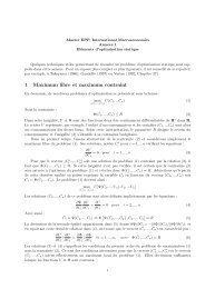
Figure 1: U.S., Terms of Trade and Trade-Weighted Real Exchange Rates
0
Manufacturing PPI-based RER
-5
Manufacturing Terms of Trade
Tradeables CPI-based RER
-10
-15
% cumulative change
-20
-25
-30
-35
-40
-45
1986 1988 1990 1992 1994 1996 1998 2000 2002 2004 2006
Sources: Manufactured X and M price indices from the BLS. RERs defined as US price over
Source of data: BLS, Source OECD, and various national statistical agencies. See data appendix for details.
a trade-weighted average of the US trading partners’ prices. PPIs cover manufactured goods
and CPIs exclude services
ToTs are less volatile than PPI-RERs (σ ToT /σ PPI = 1/3 − 2/3)
Fluctuations in CPI-based RERs are roughly as large as for PPI-RERs
Atkeson & Burstein
GT CREST-LMA

Introduction
Model
Simulation of the model
Conclusion
Empirical motivation (3)
StDev relative to PPI /PPI ∗ Correlation with PPI /PPI ∗
PPI /EPI IPI /PPI ∗ PPI /EPI IPI /PPI ∗
USA .32 .67 .45 .82
Japan .53 .42 .87 .72
Germany .38 .69 .24 .70
France .64 .66 .70 .70
Italy .69 .72 .59 .54
UK .44 .63 .62 .86
Canada .50 .57 .63 .53
Deviations from relative PPP are 1/3 to 2/3 as large as fluctuations in
PPI-RERs and positively correlated with movements in the PPI-RER
Deviations from relative PPP also observed in disaggregated data (but
heterogeneity across sectors)
Atkeson & Burstein
GT CREST-LMA

Objective
Introduction
Model
Simulation of the model
Conclusion
Build a model of international trade and international relative prices
to account for these aggregate price observations
Deviations from aggregate relative PPP as a result of the decisions
of individual firms to PTM
Key ingredients:
Imperfect competition with variable markups (Quantity competition
à la Cournot → Markups depend on market shares) → Incentive to
price-to-market
International trade costs → Ability to price-to-market and impact on
optimal markups
Calibrate the model using data on trade volumes and market
structures
Atkeson & Burstein
GT CREST-LMA

Main results
Introduction
Model
Simulation of the model
Conclusion
Firms price-to-market in response to aggregate shocks
Large firms are more prone to PTM → At the aggregate level,
pass-through is lower in sectors with a high dispersion of costs.
Calibration results show that the model is able to reproduce
i) movements in the ToTs that are smaller than corresponding
movements in the PPI-based RER for manufactures, and
ii) movements in the CPI-based RER that are similar to corresponding
movements in the PPI-based RER.
Both variable markups and international trade costs are crucial in
generating these results:
Without variable markups, shocks to the marginal cost of production
leave the ratio of export to producer prices unchanged
Without international trade costs, the extent of competition is
identical in both markets and markups move identically following a
cost shock
International trade costs also justify imports form a small share of
the CPI, which is at the root of the good match of CPI and PPI
volatilities.
Atkeson & Burstein
GT CREST-LMA

Introduction
Model
Simulation of the model
Conclusion
Hypotheses of the model: Households
Two symmetric countries (indexed by i = 1, 2) produce and trade a
continuum of goods subject to frictions in international goods
markets.
Aggregate shocks to productivity as the driving force behind
fluctuations in international relative prices.
Preferences in country i:
∑
∞
E 0
t=0
β t u(c it , 1 − l it )
where β is the discount factor, and u(c, 1 − l) = log[c µ (1 − l) 1−µ ]
with c it final consumption and l it working hours of the representative
household.
Households in each country trade a complete set of international
assets ⇒ Nominal consumptions are always equalized across
countries.
Atkeson & Burstein
GT CREST-LMA

Introduction
Model
Simulation of the model
Conclusion
Hypotheses of the model: Firms
In each country i and sector j, there are K domestic firms and an
additional K foreign firms that may, in equilibrium, sell goods in that
sector. Firms k ∈ [1, K] are domestic and k ∈ [K + 1, 2K] are
foreign. K taken as exogenous (no decision to enter the market) and
assumed small (oligopolistic competition).
Output in each sector is given by:
y ijt =
[ 2K∑
k=1
q
ρ−1
ρ
ijkt
] ρ
ρ−1
, ρ < ∞
where q ijkt denotes sales in country i of firm k in sector j.
Sectors are then further aggregated into a consumption composite,
produced by a competitive firm using the output of sectors as input:
[∫ 1
c it =
0
η−1
η
yijt
] η
η−1
dj , 1 < η < ρ
Atkeson & Burstein
GT CREST-LMA

Introduction
Model
Simulation of the model
Conclusion
Hypotheses of the model: Firms (2)
Each firm has a constant returns to scale production function that
has labor as the only input:
y ikt = A it z k l ikt
where z k differs across firms but is fixed over time and A it denotes
aggregate productivity that affects all firms based in country i. z is
drawn from a log-normal distribution, N(0, θ) (sector-specific).
In addition to the production costs, there are costs of international
trade:
International trade is prohibitively costly for final consumption.
The output of firms can be traded, under two type of costs: a fixed
labor cost F to export and an iceberg type marginal cost of
exporting τ.
Firms play a static game of quantity competition: choose quantities
q ijkt taking as given the quantities chosen by other firms, the
domestic wage W i , the final consumption price P i and the aggregate
quantity c i but recognizing that sectoral prices P ij and quantities y ij
are endogenous to their choice.
Atkeson & Burstein
GT CREST-LMA

Introduction
Model
Simulation of the model
Conclusion
Household’s program
{ maxcis ,l is ,b is+1
E 0
∑ ∞
t=0 βt u(c it , 1 − l it )
u.c.
P it c it + b it+1 = W it l it + (1 + r)b it
⇒ Intratemporal arbitrage condition between consumption and leisure:
⇒ Euler equation:
1 − µ
µ
c it
1 − l it
= W it
P it
β P it
P it+1
(1 + r)u ′ c(c it+1 , 1 − l it+1 ) = u ′ c(c it , 1 − l it )
⇒ Under complete markets:
P 1t c 1t = P 2t c 2t
Atkeson & Burstein
GT CREST-LMA

Introduction
Model
Simulation of the model
Conclusion
Optimal demands
At the sectoral level:
Max c it s.t. budget constraint
⇒ y ijt =
At the firm level:
Max y ijt s.t. budget constraint
(
Pijt
[∫ 1
P it =
⇒ q ijkt =
P ijt =
P it
) −η
c it
0
P 1−η
ijt
dj
] 1
1−η
(
Pijkt
P ijt
) −ρ
y ijt
[ 2K∑
k=1
P 1−ρ
ijkt
] 1
1−ρ
Atkeson & Burstein
GT CREST-LMA

Introduction
Model
Simulation of the model
Conclusion
Firms’ behaviour without trade
Suppose for now that only the K domestic firms in each
country/sector sell goods
Equilibrium prices and quantities obtained from:
⎧
]
max Pijkt ,q ijkt
[P ijkt q ijkt − W it
z k A it
q ijkt
Optimal prices:
where s ijkt ≡
⎪⎨
⎪⎩
s.t.
country i and ε(s ijkt ) ≡
P ijkt
P it
=
(
qijkt
) −1/ρ (
yijt
y ijt
[ ∑
ρ−1
y ijt =
k q ρ
ijkt
ε(s ijkt)
c it
) −1/η
] ρ
ρ−1
W it
P ijkt =
ε(s ijkt ) − 1 z k A it
P ijktq ijkt
Pk P ijktq ijkt
= dy ijt/y ijt
dq ijkt /q ijkt
elasticity of demand.
Optimal quantities come immediately
is the firm’s market share in
[
−1
1
ρ (1 − s ijkt) + 1 η ijkt] s is the perceived
Atkeson & Burstein
GT CREST-LMA

Introduction
Model
Simulation of the model
Conclusion
Firms’ behaviour without trade (2)
Limit cases:
K → ∞ ⇒ s → 0 ⇒ ε(s) = ρ: the firm only perceives the sectoral
elasticity of demand ρ and chooses a markup equal to ρ/(ρ − 1).
s → 1 ⇒ ε(s) = η: the firm only perceives the (lower) elasticity of
demand across sectors and sets a higher markup equal to η/(η − 1)
η = ρ: the model reduces to the standard model of monopolistic
competition with a constant markup of price over marginal cost
given by ρ/(ρ − 1) (Ghironi & Mélitz, 2005).
When ρ > η, firms with a sectoral market share between zero and
one choose a markup that increases smoothly with that market share
(rq: idem under Bertrand competition).
⇒ Prices and costs are not linearly related in the model → incomplete
pass-through of changes in cost: an increase in a firm’s relative
marginal cost induces a market share loss and a markup reduction.
⇒ PTM will naturally arise if a change in costs for one firm leads to a
change in markups that is different in each market in which this firm
competes → Requires international trade costs (lower market share
in the export market)
Atkeson & Burstein
GT CREST-LMA

Export decisions
Introduction
Model
Simulation of the model
Conclusion
To determine how many foreign firms pay the fixed trade cost to
supply the domestic market, an iterative procedure is used: foreign
firms consider entry sequentially in reverse order of unit costs (the
lowest cost producer k + 1 enters, if it still makes profits, the second
lowest cost producer k + 2 enters, etc.)
Optimal price of the lowest cost foreign firm:
P ijK+1t =
ε(s ijK+1t) τW i ′ t
ε(s ijK+1t ) − 1 z K+1 A i ′ t
⇒ Used to compute the sectoral quantity and price and the demand
addressed to the firm → Expected profits from foreign sales →
Entry if profits are higher than the fixed cost W i ′
tF
if her aggregate profit is strictly positive, the second lowest cost
producer is likely to enter market i as well.
⇒ Iterating over firms gives a set of equilibrium prices P ijkt and a
number of foreign firms supplying the domestic market in sector j,
given fixed aggregate prices, wages, and quantities.
Atkeson & Burstein
GT CREST-LMA

Introduction
Model
Simulation of the model
Conclusion
General equilibrium
W 2 chosen as numéraire
1. Solve for the number of firms and prices in every sector in both
countries for given P 1 , P 2 , c 1 , c 2 and W 1
2. Use individual prices to get aggregate and sectoral prices
3. Use quantities produced by each firm and the amount of fixed costs
to get aggregate labor demand
4. Combine the labor-market equilibrium together with the household’s
first order conditions to get a fixed point in the aggregate variables
{P i , W i , c i , l i } 2 i=1
Atkeson & Burstein
GT CREST-LMA

Calibration
Introduction
Model
Simulation of the model
Conclusion
Objective: Study the response of international relative prices to an
exogenous shock to aggregate productivity in a calibrated version of
the model
Parameters of the utility function set at standard values: β = .96,
µ = 2/3
20,000 sectors (more disaggregated than the 10-digit level of the
NAICS nomenclature) and 20 firms per sector
η ≃ 1 (Cobb-Douglas), ρ = 10
θ, τ and F matching observations in the US economy on the overall
volume of trade, the fraction of firms that export and a measure of
industry concentration at the sectoral level (symmetric equilibrium
A 1 = A 2 ): θ = .385, τ = 1.45, share of labor force in export fixed
effects=.08%
Atkeson & Burstein
GT CREST-LMA

Calibration (2)
Introduction
Model
Simulation of the model
Conclusion
Alternative parameter settings: i) ρ = η = 3 (constant markups), ii)
τ = 1 and F = 0 (frictionless trade)
Shock: one percent increase in relative aggregate costs
(W 1 /A 1 )/(W 2 /A 2 )
Construct sectoral and aggregate PPI, IPI, EPI, CPI: price indices
using the predicted sales (or expenditures) as weights
Remark: Treat the problem of extensive effects by attributing a price
change equal to the overall change in the index for goods that
switch export or import status as a result of the shock
Atkeson & Burstein
GT CREST-LMA

Introduction
Model
Simulation of the model
Conclusion
Calibration results
Table: Impact of a 1% shock on relative production costs
Complete Constant Frictionless
Model Markups Trade
PPI-based RER (decomposition %)
Terms-of-trade, country 1 53.4% 100% 100%
PPI/Export price, country 1 23.1% 0% 0%
Export price/PPI, country 2 23.6% 0% 0%
PPI, country 1 0.86% 1% 0.76%
Export price, country 1 0.69% 1% 0.76%
Import price, country 1 0.31% 0% 0.23%
PPI, country 2 0.14% 0% 0.23%
CPI-RER/PPI-RER 82.3% 66.9% 0%
Source: Atkeson & Burstein (2008). Benchmark calibration.
Atkeson & Burstein
GT CREST-LMA

Introduction
Model
Simulation of the model
Conclusion
Calibration results (2): Terms-of-Trade
Movements in the ToT are 53% as large as movements in the
PPI-RER ⇒ Reproduces the first fact
Explanation: Large deviations from relative PPP due to individual
decisions to PTM: g PPI > g EPI and g IPI > g PPI ∗⇒ Positive
correlation in the movements of PPI /EPI and IPI /PPI ∗ with
PPI /PPI ∗
Both variable markups and trade costs are necessary to get this
result:
Constant markups → Complete pass-through → Relative PPP at the
good level and no impact at the extensive margin
Frictionless trade → market shares are identical in the domestic and
foreign markets and all firms serve both markets → Incomplete
pass-through but equal in both countries → No PTM
Atkeson & Burstein
GT CREST-LMA

Introduction
Model
Simulation of the model
Conclusion
Calibration results (3): CPI-based RER
Movements in the CPI-based RER are 83% as large as movements in
the PPI-based RER
Explanation: Low (calibrated) share of imports + deviations from
relative PPP
Relative volatility of CPI-RERs much lower in the constant markups
and the frictionless trade models:
Frictionless trade: relative PPP + identical consumption baskets
(s M = .5) → CPI-based RER does not move at all
Constant markups: relative PPP but different consumption baskets
(s M = .165) → Movements in the CPI-based RER are 67% as large
as movements in the PPI-based RER
Atkeson & Burstein
GT CREST-LMA

Introduction
Model
Simulation of the model
Conclusion
Adding non-traded distribution costs
In the simulation, the relative volatility of the CPI-based RER w.r.t.
the PPI-based RER is still too low
⇒ Solution: Add non-tradeable distribution costs to reduce the share of
traded goods in the CPI
Final consumption requires adding distribution services in the form
of non-tradeable goods (labor inputs in the model):
[∫ 1 (
c it =
0
y 1−φ
ijt
d φ
ijt
) η−1
η
] η
η−1
dj , 1 < η < ρ
⇒ Distribution costs account for a constant share of retail prices for
each individual good → Do not change PTM behaviors
When φ is calibrated to 0.5, changes in the CPI-based RER are
111% as large as changes in the PPI-based RER
Role of distribution costs: Reduce s M + Amplify fluctuations in CPIs
as fluctuations in the relative price of distribution are larger than
fluctuations in the PPI-based RER (no incomplete pass-through)
Atkeson & Burstein
GT CREST-LMA

Introduction
Model
Simulation of the model
Conclusion
Individual PTM behaviors
Firms PTM by adjusting their markup to changes in their market
share
⇒ Extent of PTM depends on the exact configuration of costs across
firms in the sector
⇒ Productivity heterogeneity generates price heterogeneity
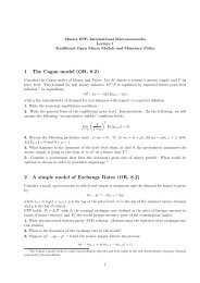
In the simulations, PPI raises in comparison to EPI because large
firms PTM and dominate the index
Atkeson & Burstein
GT CREST-LMA

Introduction
Model
Simulation of the model
Conclusion
Individual PTM behaviors (2)
Sources: Atkeson & Burstein (2008). Simulation of a 1% increase in country 1’s productivity
Atkeson & Burstein
GT CREST-LMA

Introduction
Model
Simulation of the model
Conclusion
Individual PTM behaviors (3)
More productive firms are more prone to PTM:
ˆP 1k − ˆP 2k = Γ(s 1k )ŝ 1k − Γ(s 2k )ŝ
2k
1
=
1 + Γ(s 1k )(ρ − 1) − 1
(ŵ 1k − ˆP 1) + Γ(s 2k (ρ − 1)
1 + Γ(s 2k )(ρ − 1)
1 + Γ(s 2k )(ρ − 1) (ˆP 1 − ˆP 2)
where Γ(s 1k ) is the elasticity of the markup w.r.t. market share,
which is increasing and convex on s
The first term captures the direct effect of a change in the firm’s
costs and induces a relative raise in the firm’s export (as s 1k > s 2k
⇒ Γ(s 1k ) > Γ(s 2k ))
The second term captures the indirect effect coming from strategic
interactions between firms which induces a relative drop in the firm’s
export: As the foreign sectoral price decreases w.r.t. the domestic
price, the firm reduces its foreign markup
The second effect dominates for more productive firms
Atkeson & Burstein
GT CREST-LMA

Introduction
Model
Simulation of the model
Conclusion
Individual PTM behaviors (4)
Heterogeneity in PTM behaviors across firms may explain
heterogeneity in the magnitude of PT across countries and sectors
In the simulations, sectors are homogeneous except for the
configuration of cost realizations → Heterogeneity in the deviations
PPI ˆ j −EPI ˆ j
from relative PPP as measured by
PPI −PPI
: mean=14%,
∗
StDev=16%
Remark: Without heterogeneity in productivity or export
participation, PTM goes in the wrong direction: Following a relative
cost shock, firms raise export prices w.r.t. domestic prices →
negative comovement of PPI /EPI and the PPI-based RER
Atkeson & Burstein
GT CREST-LMA

Introduction
Model
Simulation of the model
Conclusion
Sensitivity analysis
Increasing the number of firms per sector:
Does not necessarily reduce PPP deviations as the productivities of
the few more productive must grow to match evidence on the
Herfindahl index
Reducing the gap between ρ and η:
Reduces aggregate deviations from relative PPP but international
price moveme,ts are still substantial
Using an exponential distribution of productivities (Eaton &
Kortum, 2002):
Movements in the ToT are smoother
Variant with no variable trade cost but home bias in consumption:
Similar implications
Atkeson & Burstein
GT CREST-LMA

Conclusion
Introduction
Model
Simulation of the model
Conclusion
Model that helps reproducing empirical evidence on international
relative prices
Explanation based on real factors: Firms have an incentive to PTM
under imperfect competition and costly trade ⇒ Allows reproducing
persistent deviations from PPP (≠ PTM models based on price
stickiness)
Structure of the model may be used to analyze other sources of
international relative cost shocks (monetary shocks with nominal
rigidities, limited participation, etc.)
In the model, optimal PTM is obtained thanks to oligopolistic
competition between heterogeneous firms → Possible testable
predictions using firm-level data
Atkeson & Burstein
GT CREST-LMA