Numerical simulation of ice-ocean variability in the Barents Sea region
Numerical simulation of ice-ocean variability in the Barents Sea region
Numerical simulation of ice-ocean variability in the Barents Sea region

Create successful ePaper yourself
Turn your PDF publications into a flip-book with our unique Google optimized e-Paper software.
Ocean Dynamics manuscript No.<br />
(will be <strong>in</strong>serted by <strong>the</strong> editor)<br />
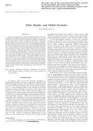
<strong>Numerical</strong> <strong>simulation</strong> <strong>of</strong> <strong>ice</strong>-<strong>ocean</strong> <strong>variability</strong> <strong>in</strong> <strong>the</strong> <strong>Barents</strong> <strong>Sea</strong><br />
<strong>region</strong><br />
Towards dynamical downscal<strong>in</strong>g<br />
W.P. Budgell<br />
Institute <strong>of</strong> Mar<strong>in</strong>e Research and Bjerknes Centre for Climate Research, Postboks 1870, Nordnes, 5817 Bergen, Norway<br />
e-mail: paul.budgell@imr.no<br />
Received: 17 December 2004<br />
Abstract. A dynamic-<strong>the</strong>rmodynamic sea <strong>ice</strong> model has<br />
been coupled to a three-dimensional <strong>ocean</strong> general circulation<br />
model for <strong>the</strong> purpose <strong>of</strong> conduct<strong>in</strong>g climate dynamical<br />
downscal<strong>in</strong>g experiments for <strong>the</strong> <strong>Barents</strong> <strong>Sea</strong> <strong>region</strong>. To assess<br />
model performance and suitability for such an application,<br />
<strong>the</strong> coupled model has been used to conduct a h<strong>in</strong>dcast<br />
for <strong>the</strong> period 1990–2002. A comparison with available observations<br />
shows that <strong>the</strong> model successfully tracks seasonal<br />
and <strong>in</strong>terannual <strong>variability</strong> <strong>in</strong> <strong>the</strong> <strong>ocean</strong> temperature field and<br />
that <strong>the</strong> simulated horizontal and vertical distribution <strong>of</strong> temperature<br />
are <strong>in</strong> good agreement with observations. The model<br />
results follow <strong>the</strong> seasonal and <strong>in</strong>terannual <strong>variability</strong> <strong>in</strong> sea<br />
<strong>ice</strong> cover <strong>in</strong> <strong>the</strong> <strong>the</strong> <strong>region</strong>, with <strong>the</strong> exception that <strong>the</strong> model<br />
results show too much <strong>ice</strong> melt<strong>in</strong>g <strong>in</strong> <strong>the</strong> nor<strong>the</strong>rn <strong>Barents</strong> <strong>Sea</strong><br />
dur<strong>in</strong>g summer. The spatial distribution <strong>of</strong> <strong>the</strong> w<strong>in</strong>ter simulated<br />
sea <strong>ice</strong> cover is <strong>in</strong> close agreement with observations.<br />
Salt release dur<strong>in</strong>g <strong>the</strong> freez<strong>in</strong>g process <strong>in</strong> <strong>the</strong> numerical <strong>simulation</strong><br />
exhibits considerable <strong>in</strong>terannual <strong>variability</strong> and tends<br />
to vary <strong>in</strong> an opposite manner to <strong>the</strong> net <strong>in</strong>flow volume flux at<br />
<strong>the</strong> western entrance <strong>of</strong> <strong>the</strong> <strong>Barents</strong> <strong>Sea</strong>. Overall, <strong>the</strong> model<br />
produces realistic <strong>ice</strong>-<strong>ocean</strong> seasonal and <strong>in</strong>terannual <strong>variability</strong><br />
and should prove to be a useful tool for dynamical<br />
downscal<strong>in</strong>g applications.<br />
Key words. Ice-<strong>ocean</strong> model Comparison model-data <strong>Barents</strong><br />
<strong>Sea</strong><br />
climate change on <strong>the</strong> <strong>Barents</strong> <strong>Sea</strong> <strong>region</strong>, a dynamical downscal<strong>in</strong>g<br />
exercise has been <strong>in</strong>itiated as part <strong>of</strong> <strong>the</strong> Research<br />
Council <strong>of</strong> Norway’s RegClim (Regional Climate development<br />
under global warm<strong>in</strong>g) programme. Dynamical downscal<strong>in</strong>g<br />
is <strong>the</strong> production <strong>of</strong> high temporal and spatial resolution<br />
climate forecasts us<strong>in</strong>g <strong>region</strong>al models to ’downscale’<br />
coarsely-resolved global climate model results. In this case, a<br />
<strong>region</strong>al coupled <strong>ice</strong>-<strong>ocean</strong> model will be used to study future<br />
climate change scenarios <strong>in</strong> <strong>the</strong> <strong>Barents</strong> <strong>Sea</strong> based on results<br />
from <strong>the</strong> global Bergen Climate Model (Furevik et al., 2003).<br />
However, before future <strong>region</strong>al climate regimes can be simulated,<br />
it is necessary to demonstrate that <strong>the</strong> downscal<strong>in</strong>g<br />
model can reproduce current climate conditions with realistic<br />
seasonal and <strong>in</strong>terannual <strong>variability</strong>. That is <strong>the</strong> ma<strong>in</strong> goal <strong>of</strong><br />
this paper.<br />
Section 2 provides a description <strong>of</strong> <strong>the</strong> coupled <strong>ice</strong><strong>ocean</strong><br />
model toge<strong>the</strong>r with <strong>the</strong> configuration <strong>of</strong> <strong>the</strong> large-area<br />
(bas<strong>in</strong>-scale) and nested (<strong>region</strong>al-scale) models. The boundary<br />
and <strong>in</strong>itial conditions are def<strong>in</strong>ed and <strong>the</strong> surface forc<strong>in</strong>g<br />
fields used <strong>in</strong> <strong>the</strong> models are discussed. Section 3 conta<strong>in</strong>s<br />
<strong>the</strong> results <strong>of</strong> <strong>the</strong> validation <strong>of</strong> <strong>the</strong> <strong>region</strong>al model aga<strong>in</strong>st observations.<br />
Comparisons <strong>of</strong> model results with satellite imagery,<br />
hydrographic sections and spatially-<strong>in</strong>tegrated time series<br />
are provided. Section 4 <strong>of</strong>fers examples <strong>of</strong> <strong>the</strong> results <strong>of</strong><br />
<strong>ice</strong>-<strong>ocean</strong> <strong>in</strong>teraction <strong>in</strong> <strong>the</strong> <strong>Barents</strong> <strong>Sea</strong>. Br<strong>in</strong>e formation and<br />
meltwater production are illustrated and discussed. F<strong>in</strong>ally,<br />
<strong>the</strong> paper concludes <strong>in</strong> Section 5 with a summary and discussion<br />
<strong>of</strong> results.<br />
2 The <strong>ice</strong>-<strong>ocean</strong> model<br />
1 Introduction<br />
The <strong>Barents</strong> <strong>Sea</strong> (Figs 1 and 2), l<strong>in</strong>k<strong>in</strong>g <strong>the</strong> Nordic <strong>Sea</strong>s with<br />
<strong>the</strong> Arctic Ocean, is an important fisheries <strong>region</strong> (Sakshaug<br />
et al., 1994). The climate <strong>variability</strong> <strong>of</strong> <strong>the</strong> <strong>Barents</strong> <strong>Sea</strong> has a<br />
strong <strong>in</strong>fluence on reproduction, recruitment (Sætersdal and<br />
Loeng, 1987; Ellertsen et al., 1989), growth and distribution<br />
(Nakken and Raknes, 1987; Michalsen et al., 1998) <strong>of</strong> fish<br />
species <strong>in</strong> <strong>the</strong> <strong>region</strong>. To address <strong>the</strong> implications <strong>of</strong> future<br />
Several model studies <strong>of</strong> circulation <strong>in</strong> <strong>the</strong> <strong>Barents</strong> <strong>Sea</strong> <strong>region</strong><br />
have been carried out over <strong>the</strong> past decade or so, <strong>in</strong>clud<strong>in</strong>g<br />
those <strong>of</strong> Ådlandsvik and Loeng (1991), Stolehansen and<br />
Slagstad (1991), Harms (1992), Loeng et al. (1997), Harms<br />
(1997), Ådlandsvik and Hansen (1998), Aspl<strong>in</strong> et al. (1998),<br />
Ingvaldsen et al. (2004a) and Maslowski et al. (2004). The<br />
current study is based on a new <strong>ice</strong>-<strong>ocean</strong> model system run<br />
at high spatial resolution for a multi-year <strong>simulation</strong> validated<br />
aga<strong>in</strong>st available observations.
2<br />
120<br />
S<br />
N<br />
70<br />
F<br />
V<br />
0<br />
K<br />
60<br />
80<br />
60<br />
40<br />
Fig. 1. <strong>Barents</strong> <strong>Sea</strong> <strong>region</strong>al model doma<strong>in</strong> show<strong>in</strong>g <strong>the</strong> location <strong>of</strong> sections: FB (Fugløya-Bjørnøya), K (Kola), V (Vardø North), S (Spitzbergen<br />
Bank) and N (West Novaya Zemlya)<br />
The <strong>ocean</strong> model component is based on ROMS (Regional<br />
Ocean Modell<strong>in</strong>g System) version 2.1. ROMS is a threedimensional<br />
barocl<strong>in</strong>ic general <strong>ocean</strong> model, <strong>the</strong> development<br />
<strong>of</strong> which is described <strong>in</strong> a series <strong>of</strong> papers (Song and<br />
Haidvogel, 1994; Haidvogel and Beckmann, 1999; Haidvogel<br />
et al., 2000; Shchepetk<strong>in</strong> and McWilliams, 2003). ROMS<br />
uses a topography-follow<strong>in</strong>g coord<strong>in</strong>ate system <strong>in</strong> <strong>the</strong> vertical<br />
that permits enhanced resolution near <strong>the</strong> surface and<br />
bottom (Song and Haidvogel, 1994). Orthogonal curvil<strong>in</strong>ear<br />
coord<strong>in</strong>ates are used <strong>in</strong> <strong>the</strong> horizontal. A spl<strong>in</strong>e expansion<br />
can be used for vertical discretization which provides<br />
for an improved representation <strong>of</strong> <strong>the</strong> barocl<strong>in</strong>ic pressure gradient<br />
(Shchepetk<strong>in</strong> and McWilliams, 2003), vertical advection<br />
and vertical diffusion <strong>of</strong> momentum and tracers. ROMS<br />
has been designed from <strong>the</strong> ground up to run efficiently <strong>in</strong><br />
both distributed (MPI) and shared (OpenMP) memory parallel<br />
comput<strong>in</strong>g environments, thus enabl<strong>in</strong>g computationally<strong>in</strong>tensive<br />
dynamical downscal<strong>in</strong>g experiments to be conducted.<br />
Fig. 2. Large-area model doma<strong>in</strong> show<strong>in</strong>g <strong>the</strong> location <strong>of</strong> <strong>the</strong> nested<br />
<strong>Barents</strong> <strong>Sea</strong> <strong>region</strong>al model doma<strong>in</strong><br />
2.1 The <strong>ocean</strong> model component<br />
2.2 The <strong>ice</strong> model component<br />
Large portions <strong>of</strong> <strong>the</strong> <strong>Barents</strong> <strong>Sea</strong> are <strong>ice</strong>-covered for much<br />
<strong>of</strong> <strong>the</strong> year. Thus, it is important to <strong>in</strong>clude <strong>the</strong> effects <strong>of</strong> <strong>ice</strong><br />
drift, melt<strong>in</strong>g and freez<strong>in</strong>g upon <strong>the</strong> <strong>ocean</strong> fields. To accomplish<br />
this, a dynamic-<strong>the</strong>rmodynamicsea <strong>ice</strong> module has been<br />
developed and coupled to <strong>the</strong> <strong>ocean</strong> model. The <strong>ice</strong> dynamics<br />
are based upon an elastic-viscous-plastic (EVP) rheology<br />
after Hunke and Dukowicz (1997) and Hunke (2001). The<br />
EVP scheme is based on a time-splitt<strong>in</strong>g approach whereby<br />
short elastic time steps are used to regularize <strong>the</strong> solution<br />
when <strong>the</strong> <strong>ice</strong> exhibits nearly rigid behaviour. Because <strong>the</strong> time<br />
discretization uses explicit time-stepp<strong>in</strong>g, <strong>the</strong> <strong>ice</strong> dynamics<br />
are readily parallelizable and thus computationally efficient.<br />
Employ<strong>in</strong>g l<strong>in</strong>earization <strong>of</strong> viscosities about <strong>ice</strong> velocities at<br />
every elastic (short) time step, as recommended by Hunke
3<br />
(2001), has <strong>the</strong> desirable property <strong>of</strong> ma<strong>in</strong>ta<strong>in</strong><strong>in</strong>g <strong>the</strong> <strong>ice</strong> <strong>in</strong>ternal<br />
stress state on or <strong>in</strong> <strong>the</strong> plastic yield curve. That is, <strong>the</strong><br />
<strong>ice</strong> deforms as a plastic material unless it is <strong>in</strong> a rigid state.<br />
Ano<strong>the</strong>r desirable property <strong>of</strong> <strong>the</strong> Hunke (2001) l<strong>in</strong>earization<br />
is that <strong>the</strong> EVP <strong>ice</strong> dynmamics are found to provide a good<br />
transient response to rapidly vary<strong>in</strong>g w<strong>in</strong>ds as well as to <strong>in</strong>ertial<br />
and tidal dynamics, particularly <strong>in</strong> <strong>the</strong> marg<strong>in</strong>al <strong>ice</strong> zone.<br />
The <strong>ice</strong> <strong>the</strong>rmodynamics are based on those <strong>of</strong> Mellor and<br />
Kantha (1989) and Häkk<strong>in</strong>en and Mellor (1992). Two <strong>ice</strong> layers<br />
and a s<strong>in</strong>gle snow layer are used <strong>in</strong> solv<strong>in</strong>g <strong>the</strong> heat conduction<br />
equation. The snow layer possesses no heat content,<br />
but is, <strong>in</strong> effect, an <strong>in</strong>sulat<strong>in</strong>g layer. Surface melt ponds are<br />
<strong>in</strong>cluded <strong>in</strong> <strong>the</strong> <strong>ice</strong> <strong>the</strong>rmodynamics. A molecular sub-layer<br />
(Mellor et al., 1989) separates <strong>the</strong> bottom <strong>of</strong> <strong>the</strong> <strong>ice</strong> cover<br />
from <strong>the</strong> upper <strong>ocean</strong>. The <strong>in</strong>clusion <strong>of</strong> <strong>the</strong> molecular sublayer<br />
was found to produce much more realistic freez<strong>in</strong>g and<br />
melt<strong>in</strong>g rates than if <strong>the</strong> <strong>ice</strong>-<strong>ocean</strong> heat flux is based purely<br />
on <strong>the</strong> <strong>ice</strong> bottom - <strong>ocean</strong> upper layer temperature difference.<br />
2.3 The Large-Area model<br />
The large-area model (Fig 2) is used to supply boundary and<br />
<strong>in</strong>itial conditions to <strong>the</strong> <strong>region</strong>al <strong>Barents</strong> model. A stretched<br />
spherical coord<strong>in</strong>ate grid (Bentsen et al., 1999) is used <strong>in</strong> <strong>the</strong><br />
horizontal, with <strong>the</strong> North Pole situated <strong>in</strong> central Asia and<br />
<strong>the</strong> South Pole situated <strong>in</strong> <strong>the</strong> Pacific Ocean west <strong>of</strong> North<br />
America. In <strong>the</strong> <strong>Barents</strong> <strong>Sea</strong> <strong>region</strong>, <strong>the</strong> horizontal resolution<br />
is approximately 50 km. There were 30 generalized ¡ -<br />
coord<strong>in</strong>ate (¢ ) levels, stretched to <strong>in</strong>crease vertical resolution<br />
near <strong>the</strong> surface and bottom.<br />
A time step <strong>of</strong> 1800 s was used for both <strong>the</strong> <strong>ocean</strong> <strong>in</strong>ternal<br />
mode and <strong>ice</strong> <strong>the</strong>rmodynamic time step. A ratio <strong>of</strong> 40<br />
was used between <strong>the</strong> <strong>ocean</strong> <strong>in</strong>ternal and external mode time<br />
steps. A ratio <strong>of</strong> 60 was used between <strong>ice</strong> <strong>the</strong>rmodynamic and<br />
dynamic time steps.<br />
No tides were <strong>in</strong>cluded <strong>in</strong> <strong>the</strong> <strong>simulation</strong>. The vertical<br />
mix<strong>in</strong>g scheme employed was <strong>the</strong> LMD (Large et al., 1994)<br />
parameterization. The lateral boundaries were closed with <strong>the</strong><br />
exception that a constant volume flux <strong>of</strong> 1 Sv was <strong>in</strong>put across<br />
Ber<strong>in</strong>g Strait and <strong>the</strong> same quantity was removed along <strong>the</strong><br />
sou<strong>the</strong>rn boundary.<br />
The atmospheric forc<strong>in</strong>g was obta<strong>in</strong>ed from <strong>the</strong><br />
NCEP/NCAR reanalysis data (Kalnay et al., 1996). Daily<br />
mean w<strong>in</strong>d stress, and latent, sensible, downward shortwave<br />
radiative and net longwave radiative heat fluxes were applied<br />
as surface forc<strong>in</strong>g after correct<strong>in</strong>g for differences <strong>in</strong> model<br />
and NCEP surface conditions, such as <strong>in</strong> surface temperature<br />
and <strong>ice</strong> concentration. The flux corrections applied were<br />
developed by Bentsen and Drange (2000) and provide a<br />
feedback between <strong>the</strong> model surface temperature and applied<br />
heat fluxes, thus m<strong>in</strong>imiz<strong>in</strong>g problems with drift <strong>in</strong> model<br />
surface temperatures. Precipitation was taken from <strong>the</strong> daily<br />
mean NCEP values. Snowfall was taken to be precipitation,<br />
corrected for snow density, when air temperature was less<br />
than 0 £ C. Evaporation was computed from <strong>the</strong> latent heat<br />
flux.<br />
River run<strong>of</strong>f was computed us<strong>in</strong>g <strong>the</strong> NCEP/NCAR Reanalysis<br />
daily accumulated surface run<strong>of</strong>f values over land<br />
that were routed to <strong>ocean</strong> discharge po<strong>in</strong>ts us<strong>in</strong>g <strong>the</strong> Total<br />
Run<strong>of</strong>f Integrated Pathways (TRIP) approach <strong>of</strong> Oki and Sud<br />
Fig. 3. Typical SST field from <strong>the</strong> Large-Area model, from January<br />
3, 1994<br />
Fig. 4. Typical <strong>ice</strong> concentration field from <strong>the</strong> Large-Area model,<br />
from January 3, 1994<br />
(1998). The hydrographs were modified for areas north <strong>of</strong><br />
60 £ N to account for permafrost hydrology and storage <strong>in</strong><br />
snow cover.<br />
The model was started from rest at January 1, 1948<br />
with <strong>the</strong> January mean temperature and sal<strong>in</strong>ity from <strong>the</strong><br />
Polar Hydrographic Climatology (Steele et al., 2001). Initial<br />
sea <strong>ice</strong> concentration was obta<strong>in</strong>ed from <strong>the</strong> daily mean<br />
NCEP/NCAR Reanalysis sea <strong>ice</strong> concentration for January 1,<br />
1948. Initial average <strong>ice</strong> thickness (<strong>ice</strong> volume per unit area<br />
averaged over each grid cell) was specified by multiply<strong>in</strong>g <strong>the</strong><br />
<strong>in</strong>itial <strong>ice</strong> concentration by 2 m.<br />
A <strong>simulation</strong> was <strong>the</strong>n conducted to sp<strong>in</strong> up <strong>the</strong> model<br />
over <strong>the</strong> period 1948 to <strong>the</strong> end <strong>of</strong> 1987. The model fields at<br />
0000Z January 1, 1988 were <strong>the</strong>n used as <strong>in</strong>itial conditions<br />
for a h<strong>in</strong>dcast conducted from January 1, 1948 to <strong>the</strong> end <strong>of</strong><br />
2003.<br />
Typical results from <strong>the</strong> Large-Area Model for sea surface<br />
temperature (SST) and <strong>ice</strong> concentration at January 3, 1994<br />
are shown <strong>in</strong> Figs 3 and 4, respectively.
4<br />
The <strong>region</strong>al model doma<strong>in</strong> is shown <strong>in</strong> Fig 1. The <strong>region</strong>al<br />
model uses <strong>the</strong> same horizontal coord<strong>in</strong>ate system as <strong>the</strong><br />
Large-Area model, but at higher spatial resolution. The horizontal<br />
grid size varies between 7.8 and 10.5 km, with an average<br />
<strong>of</strong> 9.3 km. In <strong>the</strong> vertical, 32 s-coord<strong>in</strong>ate levels are used,<br />
with enhanced resolution near <strong>the</strong> surface and bottom.<br />
The time step used <strong>in</strong> <strong>the</strong> <strong>simulation</strong> was 450 s for both <strong>the</strong><br />
<strong>ocean</strong> <strong>in</strong>ternal mode and <strong>the</strong> <strong>ice</strong> <strong>the</strong>rmodynamics. The <strong>ocean</strong><br />
model is split mode explicit. The ratio <strong>of</strong> <strong>ocean</strong> <strong>in</strong>ternal to<br />
external mode time step is 45. The ratio <strong>of</strong> <strong>ice</strong> <strong>the</strong>rmodynamic<br />
to dynamic time step is 60.<br />
Fla<strong>the</strong>r (1976) and Chapman (1985) radiation open<br />
boundary conditions were prescribed for barotropic normal<br />
velocity components and <strong>the</strong> free surface, respectively. Flow<br />
relaxation scheme (Engedahl, 1995) open boundary conditions<br />
were employed for three-dimensional velocity components<br />
and tracers. The <strong>region</strong>al model was forced at <strong>the</strong><br />
boundaries with <strong>in</strong>terpolated 5-day mean fields from <strong>the</strong><br />
Large-Area model and with tidal velocities and free surface<br />
heights from 8 constituents <strong>of</strong> <strong>the</strong> Arctic Ocean Tidal Inverse<br />
Model (AOTIM) by Padman and Er<strong>of</strong>eeva (2004).<br />
Surface forc<strong>in</strong>g for <strong>the</strong> <strong>region</strong>al model was <strong>the</strong> same<br />
as that applied <strong>in</strong> <strong>the</strong> Large-Area model <strong>simulation</strong>s and<br />
described <strong>in</strong> section 2.3, but with <strong>the</strong> exception that <strong>the</strong><br />
NCEP/NCAR Reanalysis cloud cover fraction was modified<br />
to provide <strong>the</strong> same monthly mean cloud cover climatology<br />
over <strong>the</strong> period 1983–2002 as <strong>the</strong> International Satellite<br />
Cloud Climatology Project (ISCCP) cloud cover data (Schiffer<br />
and Rossow, 1985). This necessitated <strong>the</strong> modification <strong>of</strong><br />
<strong>the</strong> downward shortwave radiation and net longwave radiation<br />
fluxes to be consistent with <strong>the</strong> new cloud data. In <strong>the</strong><br />
first <strong>simulation</strong>s <strong>of</strong> <strong>Barents</strong> <strong>Sea</strong> <strong>ice</strong> cover, we found excessive<br />
melt<strong>in</strong>g <strong>of</strong> sea <strong>ice</strong> <strong>in</strong> summer by shortwave radiation due<br />
to <strong>the</strong> NCEP/NCAR Reanalysis cloud cover fraction be<strong>in</strong>g<br />
too low by a factor <strong>of</strong> approximately 0.75. This problem was<br />
largely, but not entirely, remedied by <strong>the</strong> use <strong>of</strong> ISCCP cloud<br />
cover data.<br />
Initial copnditions for <strong>the</strong> <strong>Barents</strong> <strong>region</strong>al model were<br />
obta<strong>in</strong>ed from <strong>the</strong> archived 5-day mean Large-Area model<br />
fields <strong>in</strong>terpolated to January 1, 1990. The <strong>Barents</strong> <strong>simulation</strong><br />
was conducted for <strong>the</strong> period 1990–2002.<br />
3 Model-data comparison<br />
Fig. 5. Typical sea surface height field from <strong>the</strong> Large-Area model,<br />
from January 3, 1994<br />
From <strong>the</strong> map <strong>of</strong> sea surface height from <strong>the</strong> Large-Area<br />
model on <strong>the</strong> same date shown <strong>in</strong> Fig 5, it can be seen that<br />
even though <strong>the</strong> model resolution <strong>in</strong> <strong>the</strong> Gulf Stream <strong>region</strong><br />
<strong>in</strong> <strong>the</strong> western Atlantic is coarse at ¤ 80 km, <strong>the</strong> Gulf Stream<br />
separates from <strong>the</strong> western boundary at <strong>the</strong> correct location -<br />
Cape Hatteras, 35 £ N. The bas<strong>in</strong>-scale circulation and temperature<br />
patterns are realistic and are suitable for use <strong>in</strong> boundary<br />
forc<strong>in</strong>g <strong>of</strong> <strong>the</strong> <strong>region</strong>al model.<br />
2.4 The <strong>Barents</strong> <strong>region</strong>al model<br />
Model results are compared with data from a variety <strong>of</strong><br />
sources, <strong>in</strong>clud<strong>in</strong>g satellite SST and passive micowave, hydrographic<br />
sections and time series <strong>of</strong> <strong>in</strong>tegral quantities.<br />
3.1 Ocean data<br />
3.1.1 Satellite SST An <strong>in</strong>dication <strong>of</strong> <strong>the</strong> spatial structure <strong>of</strong><br />
<strong>the</strong> sea surface temperature can be obta<strong>in</strong>ed from SST derived<br />
from satellite Advanced Very High Resolution Radiometer<br />
(AVHRR) by <strong>the</strong> Pathf<strong>in</strong>der programme at <strong>the</strong> NASA Physical<br />
Oceanography Distributed Active Archive Center (PO-<br />
DAAC). Monthly-mean, 4-km resolution, best fields from ascend<strong>in</strong>g<br />
(day-time) orbits are compared with <strong>the</strong> correspond<strong>in</strong>g<br />
model values for March and September, 1993 <strong>in</strong> Fig 6.<br />
The PODAAC SST fields are <strong>in</strong>terpolated on to <strong>the</strong> model<br />
grid us<strong>in</strong>g nearest neighbour <strong>in</strong>terpolation.<br />
It can be seen that, <strong>in</strong> March, <strong>the</strong> model produces a realistic<br />
transport <strong>of</strong> warm water northward west <strong>of</strong> Spitzbergen<br />
<strong>in</strong> <strong>the</strong> West Spitzbergen Current and that <strong>the</strong> <strong>region</strong> encompassed<br />
by <strong>the</strong> 2 degree iso<strong>the</strong>rm matches <strong>the</strong> satellite SST<br />
distribution, but <strong>the</strong> model results are ¤ 2 degrees too cold <strong>in</strong><br />
<strong>the</strong> middle <strong>of</strong> <strong>the</strong> Norwegian <strong>Sea</strong> near <strong>the</strong> left-hand (sou<strong>the</strong>rn)<br />
boundary. The model results for September show good<br />
agreement with <strong>the</strong> satellite SST field.<br />
3.1.2 Hydrographic sections Model results were compared<br />
with two hydrographic sections: <strong>the</strong> Fugløya– Bjørnøya and<br />
Vardø North sections (sections FB and V, respectively, <strong>in</strong><br />
Fig 1). Shown <strong>in</strong> Fig 7 are modelled and observed temperatures<br />
from March <strong>in</strong> <strong>the</strong> years 1992–1994. Given that <strong>the</strong><br />
modelled fields are only averaged over a day and are compared<br />
to (¤ a 2 day) nearly-synoptic hydrographic section,<br />
<strong>the</strong> agreement is remarkably good. The model results show<br />
good placement <strong>of</strong> <strong>the</strong> Polar Front along <strong>the</strong> Bjørnøya (nor<strong>the</strong>rn)<br />
slope. The model results ¤ are 1 degree too warm at <strong>the</strong><br />
surface near Bjørnøya at <strong>the</strong> nor<strong>the</strong>rn end <strong>of</strong> <strong>the</strong> section.<br />
The results for temperatures <strong>in</strong> September are even better<br />
than those from March, as can be seen from Fig 8. The GLS<br />
mix<strong>in</strong>g scheme produces mixed layers <strong>of</strong> <strong>the</strong> right thickness<br />
dur<strong>in</strong>g <strong>the</strong> stratified late summer conditions. The modelled<br />
temperatures are still too warm <strong>in</strong> <strong>the</strong> immediate vic<strong>in</strong>ity <strong>of</strong><br />
Bjørnøya.
5<br />
Fig. 6. Modelled vs. Pathf<strong>in</strong>der AVHRR monthly-mean SST. The top row is from March, 1993, <strong>the</strong> lower row is from September, 1993. The<br />
left-hand column conta<strong>in</strong>s <strong>the</strong> model fields, <strong>the</strong> right-hand panel conta<strong>in</strong>s <strong>the</strong> Pathf<strong>in</strong>der AVHRR fields.<br />
Sal<strong>in</strong>ity is a much more difficult property to represent correctly,<br />
as can be seen from Figs 9 and 10.<br />
The modelled Atlantic Water <strong>in</strong>flow, situated roughly <strong>in</strong><br />
<strong>the</strong> middle <strong>of</strong> <strong>the</strong> section, is ¤ 0.05–0.1 too low. The modelled<br />
coastal current at <strong>the</strong> sou<strong>the</strong>rn end <strong>of</strong> <strong>the</strong> section is too<br />
narrow, and is 0.5 too sal<strong>in</strong>e. The fresher, colder Arctic Surface<br />
Water outflow jet along <strong>the</strong> slope south <strong>of</strong> Bjørnøya at<br />
<strong>the</strong> nor<strong>the</strong>rn end <strong>of</strong> <strong>the</strong> section is miss<strong>in</strong>g completely <strong>in</strong> <strong>the</strong><br />
model results. Both <strong>the</strong> temperature and sal<strong>in</strong>ity figures show<br />
that <strong>the</strong> modelled vertical structure <strong>in</strong> March tends to be more<br />
homogeneous than <strong>in</strong> <strong>the</strong> observations.<br />
A model-data comparison was also conducted for <strong>the</strong><br />
Vardø North section. Shown <strong>in</strong> Figs 11 and 12 are <strong>the</strong> modelled<br />
and observed temperatures for March and September,<br />
respectively, for 1992–1994.<br />
Aga<strong>in</strong>, <strong>the</strong> modelled temperatures are <strong>in</strong> good agreement<br />
with <strong>the</strong> observations, but at this section <strong>the</strong> agreement between<br />
modelled and observed sal<strong>in</strong>ities is much better. The<br />
model results tend to be too vertically well-mixed at <strong>the</strong><br />
sou<strong>the</strong>rn end <strong>of</strong> <strong>the</strong> section.<br />
3.1.3 Kola section time series Temperatures at <strong>the</strong> Kola section<br />
(denoted K <strong>in</strong> Fig 1), have been monitored back to 1900<br />
(Ozhig<strong>in</strong>, pers. comm.). The Kola section temperatures have<br />
been averaged over <strong>the</strong> upper 200 m and along <strong>the</strong> section<br />
between 70.5 to 72.5 £ N at 33.5 £ E. The Kola section temperature<br />
time series has been shown to be related to cod stock<br />
recruitment and is a useful <strong>in</strong>dicator <strong>of</strong> climatic <strong>variability</strong> <strong>in</strong><br />
<strong>the</strong> <strong>Barents</strong> <strong>Sea</strong> (Dippner and Ottersen, 2001). Thus, <strong>the</strong> Kola<br />
section temperature series is a good validation data set for<br />
comparison with model results. Shown <strong>in</strong> Fig 15 is a comparison<br />
<strong>of</strong> modelled and observed values <strong>of</strong> monthly mean Kola<br />
section temperatures for <strong>the</strong> period 1990–2001. A constant<br />
value <strong>of</strong> 0.7 degrees C has been subtracted from <strong>the</strong> displayed<br />
model temperatures to account for <strong>the</strong> bias <strong>of</strong> +0.66 degrees<br />
<strong>in</strong> <strong>the</strong> model results relative to <strong>the</strong> observations over <strong>the</strong> period<br />
1992–2001 (ignor<strong>in</strong>g <strong>the</strong> first two years as sp<strong>in</strong>-up).<br />
It can be seen that <strong>the</strong> model results track <strong>the</strong> seasonal and<br />
<strong>in</strong>terannual variations <strong>in</strong> <strong>the</strong> Kola section temperatures very<br />
well. The cause <strong>of</strong> <strong>the</strong> 0.66 degree bias <strong>in</strong> <strong>the</strong> model results<br />
is not clear at this time. Possible candidates <strong>in</strong>clude too high<br />
<strong>in</strong>flow <strong>of</strong> Atlantic Water and systematic errors <strong>in</strong> <strong>the</strong> radiative<br />
heat flux used to drive <strong>the</strong> model.
6<br />
Fig. 7. Modelled vs. observed temperatures from <strong>the</strong> Fugløya– Bjørnøya section for March, 1992–1994. The top row is from 1992, <strong>the</strong> middle<br />
row is from 1993 and <strong>the</strong> bottom row is from 1994. The left-hand column conta<strong>in</strong>s <strong>the</strong> daily-mean modelled temperatures, <strong>the</strong> right-hand<br />
panel conta<strong>in</strong>s <strong>the</strong> temperatures from CTD (conductivity-temperature-depth) pr<strong>of</strong>iles.<br />
3.1.4 <strong>Barents</strong> <strong>in</strong>flow The <strong>in</strong>flow <strong>of</strong> warmer Atlantic Water<br />
through <strong>the</strong> western entrance <strong>of</strong> <strong>the</strong> <strong>Barents</strong> <strong>Sea</strong> plays an important<br />
role <strong>in</strong> determ<strong>in</strong><strong>in</strong>g <strong>the</strong> temperature and <strong>ice</strong> distribution<br />
<strong>in</strong> <strong>the</strong> <strong>Barents</strong> (Ådlandsvik and Loeng, 1991; Loeng et<br />
al., 1997). Shown <strong>in</strong> Fig 16 is <strong>the</strong> net <strong>in</strong>flow volume flux<br />
across <strong>the</strong> Fugløya-Bjørnøya section. It can be seen that <strong>the</strong><br />
seasonal <strong>variability</strong> is an order <strong>of</strong> magnitude higher than <strong>the</strong><br />
<strong>in</strong>ter-annual <strong>variability</strong>.<br />
Over <strong>the</strong> period 1992–2002, <strong>the</strong> mean net volume flux <strong>of</strong><br />
<strong>in</strong>flow to <strong>the</strong> <strong>Barents</strong> across <strong>the</strong> Fugløya-Bjørnøya section is<br />
computed to be 3.2 Sv ( ¥§¦©¨¥ ). Across <strong>the</strong> full<br />
<strong>Barents</strong> entrance between nor<strong>the</strong>rn Norway and <strong>the</strong> sou<strong>the</strong>rn<br />
tip <strong>of</strong> Spitzbergen, <strong>the</strong> net <strong>in</strong>flow over <strong>the</strong> period 1992–2002<br />
is computed to be 3.6 Sv <strong>in</strong> this study. Maslowski et al. (2004)<br />
computed a value <strong>of</strong> 3.3 Sv net <strong>in</strong>flow across <strong>the</strong> same section<br />
<strong>in</strong> <strong>the</strong>ir study. From fixed current meter moor<strong>in</strong>g arrays,<br />
Ingvaldsen et al. (2004b) estimated net Atlantic Water <strong>in</strong>flow<br />
to <strong>the</strong> <strong>Barents</strong> through <strong>the</strong> Fugløya-Bjørnøya section to be<br />
1.5 Sv, averaged over <strong>the</strong> period August 1, 1997 through July<br />
31, 2001. If Atlantic Water is taken to be water warmer than<br />
3 £ C with sal<strong>in</strong>ity greater than 34.9, <strong>the</strong>n on <strong>the</strong> same section,<br />
over <strong>the</strong> same period, a value <strong>of</strong> 2.5 Sv is obta<strong>in</strong>ed <strong>in</strong> this<br />
modell<strong>in</strong>g study.<br />
3.1.5 Satellite <strong>ice</strong> concentration <strong>Sea</strong> <strong>ice</strong> concentration <strong>in</strong> <strong>the</strong><br />
<strong>Barents</strong> <strong>Sea</strong> can exhibit considerable variation both seasonally<br />
and <strong>in</strong>ter-annually (Gloersen et al., 1992). Typical <strong>ice</strong><br />
concentration distributions from <strong>the</strong> maximum and m<strong>in</strong>imum<br />
<strong>ice</strong> extent periods dur<strong>in</strong>g <strong>the</strong> year are shown <strong>in</strong> Fig 17. Given<br />
that <strong>the</strong> fields shown are daily-maen values and, thus, effectively<br />
snap shots <strong>of</strong> <strong>ice</strong> distributions, <strong>the</strong> agreement between<br />
model fields and observations is remarkably good. The SSM/I<br />
(Special Sensor Microwave/Imager) data has a spatial resolution<br />
<strong>of</strong> 25 km, whereas <strong>the</strong> model resolution is ¤ 9 km.<br />
The saltellite values are l<strong>in</strong>early <strong>in</strong>terpolated on to <strong>the</strong> model<br />
grid and will appear somewhat smoo<strong>the</strong>r than <strong>the</strong> modelled<br />
values. The modelled concentrations from March display <strong>the</strong><br />
same polynya and <strong>ice</strong> build-up locations found <strong>in</strong> <strong>the</strong> satellite<br />
imagery. The September model results are <strong>in</strong> good general<br />
agreement with <strong>the</strong> observations, but show too much <strong>ice</strong><br />
melt. The modelled <strong>ice</strong> edge is too far to <strong>the</strong> north.<br />
To obta<strong>in</strong> an <strong>in</strong>tegral estimate <strong>of</strong> model performance, <strong>the</strong><br />
monthly-mean total areal <strong>ice</strong> cover has been tabulated from<br />
model results and from SSM/I satellite data. Fig 18 shows<br />
that <strong>the</strong> model results successfully track <strong>the</strong> seasonal and<br />
<strong>in</strong>ter-annual <strong>variability</strong>, but that <strong>the</strong>re is a systematic underestimation<br />
<strong>of</strong> summer <strong>ice</strong> cover, consistent with <strong>the</strong> September<br />
results shown <strong>in</strong> Fig 17.<br />
4 Ice-<strong>ocean</strong> <strong>in</strong>teraction<br />
Ice freez<strong>in</strong>g and melt<strong>in</strong>g processes have <strong>the</strong> potential to modify<br />
water mass characteristics through br<strong>in</strong>e rejection and<br />
subsequent <strong>in</strong>termediate and deep water formation dur<strong>in</strong>g <strong>the</strong>
7<br />
Fig. 8. As <strong>in</strong> Fig 7, but for September.<br />
Fig. 9. As <strong>in</strong> Fig 7, but for sal<strong>in</strong>ity.
8<br />
Fig. 10. As <strong>in</strong> Fig 9, but for September.<br />
Fig. 11. As <strong>in</strong> Fig 7, but for Vardø North.
9<br />
Fig. 12. As <strong>in</strong> Fig 11, but for September.<br />
Fig. 13. As <strong>in</strong> Fig 11, but for sal<strong>in</strong>ity.
10<br />
Fig. 14. As <strong>in</strong> Fig 13, but for September.<br />
freez<strong>in</strong>g process and through freshen<strong>in</strong>g <strong>of</strong> surface layers dur<strong>in</strong>g<br />
<strong>the</strong> melt<strong>in</strong>g process. The total <strong>ice</strong> formation <strong>in</strong> meters <strong>of</strong><br />
<strong>ice</strong> produced for <strong>the</strong> year 1993 as estimated from <strong>the</strong> model<br />
results is shown <strong>in</strong> Fig 19. The <strong>ice</strong> production is highest<br />
along coastal polynyas <strong>in</strong> <strong>the</strong> Kara <strong>Sea</strong> and polynyas situated<br />
around <strong>the</strong> islands <strong>of</strong> <strong>the</strong> nor<strong>the</strong>rn <strong>Barents</strong>. Broad areas <strong>of</strong> <strong>ice</strong><br />
production exist <strong>in</strong> <strong>the</strong> Kara <strong>Sea</strong>, over <strong>the</strong> banks <strong>of</strong> <strong>the</strong> nor<strong>the</strong>rn<br />
half <strong>of</strong> <strong>the</strong> <strong>Barents</strong> <strong>Sea</strong> and <strong>in</strong> <strong>the</strong> White and Pechora <strong>Sea</strong>s<br />
along <strong>the</strong> south coast <strong>of</strong> <strong>the</strong> model doma<strong>in</strong>.<br />
The distribution <strong>of</strong> total <strong>ice</strong> melt for 1993, shown <strong>in</strong><br />
Fig 20, is very different from that <strong>of</strong> <strong>ice</strong> formation. While<br />
most <strong>ice</strong> melt<strong>in</strong>g occurs <strong>in</strong> a <strong>region</strong> encompass<strong>in</strong>g <strong>the</strong> summer<br />
<strong>ice</strong> edge <strong>in</strong> <strong>the</strong> nor<strong>the</strong>rn <strong>Barents</strong>, discont<strong>in</strong>uous l<strong>in</strong>es <strong>of</strong><br />
high total <strong>ice</strong> melt are distributed throughout <strong>the</strong> portion <strong>of</strong><br />
<strong>the</strong> model doma<strong>in</strong> which encounters <strong>ice</strong> cover. A sample time<br />
series <strong>of</strong> <strong>ice</strong> melt rates at at one location situation on a high<br />
<strong>ice</strong>-melt l<strong>in</strong>e is shown <strong>in</strong> Fig 21. The melt<strong>in</strong>g is concentrated<br />
<strong>in</strong> a 5–8 day period <strong>in</strong> early June, with no o<strong>the</strong>r appreciable<br />
melt activity occurr<strong>in</strong>g over <strong>the</strong> rest <strong>of</strong> <strong>the</strong> year. The rapid<br />
melt<strong>in</strong>g event corresponds to <strong>the</strong> transport <strong>of</strong> <strong>the</strong> <strong>ice</strong> edge<br />
<strong>in</strong>to surface waters previously warmed by shortwave radiation.<br />
The melt<strong>in</strong>g occurs largely through lateral ablation. As<br />
can be seen from Fig 19, <strong>the</strong> Spitzbergen Bank (section S<br />
<strong>in</strong> Fig 1) is a zone <strong>of</strong> significant <strong>ice</strong> production. When <strong>ice</strong><br />
forms, br<strong>in</strong>es are ejected. These br<strong>in</strong>es enhance <strong>the</strong> surface<br />
sal<strong>in</strong>ity and <strong>in</strong>crease <strong>the</strong> density <strong>of</strong> <strong>the</strong> surface water which<br />
<strong>the</strong>n s<strong>in</strong>ks to form a dense, sal<strong>in</strong>e layer at <strong>the</strong> bottom. The<br />
dra<strong>in</strong>age <strong>of</strong> br<strong>in</strong>e-enriched waters down <strong>the</strong> slopes <strong>of</strong> <strong>the</strong> Spitbergen<br />
Bank is shown <strong>in</strong> Fig 22. Plumes <strong>of</strong> br<strong>in</strong>e-enhanced<br />
sal<strong>in</strong>ity can be seen dra<strong>in</strong><strong>in</strong>g down both sides <strong>of</strong> <strong>the</strong> bank.<br />
The plume on <strong>the</strong> north (left) side <strong>of</strong> <strong>the</strong> bank forms a th<strong>in</strong><br />
bottom layer <strong>in</strong> <strong>the</strong> Storfjord Trough. The br<strong>in</strong>e dra<strong>in</strong>age on<br />
<strong>the</strong> south (right) side <strong>of</strong> <strong>the</strong> bank is more diffuse, due to <strong>the</strong><br />
stronger tidal mix<strong>in</strong>g on <strong>the</strong> south side. Over <strong>the</strong> shallowest<br />
portion on <strong>the</strong> bank, <strong>the</strong> water column is vertically homogeneous,<br />
with <strong>the</strong> temperature at <strong>the</strong> freez<strong>in</strong>g po<strong>in</strong>t. The warm<br />
core over <strong>the</strong> nor<strong>the</strong>rn portion <strong>of</strong> <strong>the</strong> Stordfjord Trough (far<br />
left <strong>of</strong> figure) is due to an <strong>in</strong>trusion from <strong>the</strong> West Spitzbergen<br />
Current.<br />
Ano<strong>the</strong>r high <strong>ice</strong> production <strong>region</strong> is situated west <strong>of</strong> Novaya<br />
Zemlya along section N <strong>in</strong> Fig 1. Shown <strong>in</strong> Fig 23 are<br />
<strong>the</strong> simulated daily mean temperature and sal<strong>in</strong>ity from that<br />
section for February 28, 1994. A column <strong>of</strong> br<strong>in</strong>e-enriched<br />
water is situated over <strong>the</strong> shallowest portion <strong>of</strong> <strong>the</strong> bank.<br />
O<strong>the</strong>r, weaker br<strong>in</strong>e-enhanced columns exist <strong>in</strong> deeper waters<br />
<strong>in</strong> <strong>the</strong> western (left-hand) portion <strong>of</strong> <strong>the</strong> section. The<br />
weaker columns <strong>in</strong> deeper water is attributable to <strong>the</strong> hydrostatic<br />
property <strong>of</strong> ROMS: convection is represented as a vertical<br />
mix<strong>in</strong>g process. Thus <strong>the</strong>re is likely to be more dilution <strong>of</strong><br />
br<strong>in</strong>es with<strong>in</strong> ROMS <strong>in</strong> deeper waters than occurs <strong>in</strong> nature<br />
where br<strong>in</strong>es can s<strong>in</strong>k to <strong>the</strong> bottom with much less entra<strong>in</strong>ment<br />
<strong>of</strong> surround<strong>in</strong>g water masses.<br />
Along <strong>the</strong> western slope <strong>of</strong> <strong>the</strong> ma<strong>in</strong> bank at <strong>the</strong> centre <strong>of</strong><br />
<strong>the</strong> section <strong>the</strong> last vestige <strong>of</strong> Atlantic Water <strong>in</strong>flow appears<br />
as <strong>the</strong> warmer, less sal<strong>in</strong>e core <strong>of</strong> a northward-flow<strong>in</strong>g alongslope<br />
jet.<br />
An <strong>in</strong>tegrated annual estimate <strong>of</strong> salt production from<br />
br<strong>in</strong>e rejection <strong>in</strong> <strong>the</strong> freez<strong>in</strong>g process provides a good <strong>in</strong>-
11<br />
6<br />
5.5<br />
5<br />
4.5<br />
4<br />
3.5<br />
3<br />
2.5<br />
2<br />
1990 1992 1994 1996 1998 2000 2002<br />
Fig. 15. Modelled (red) and observed (blue) monthly mean time series <strong>of</strong> <strong>the</strong> mean Kola section temperatures. Note that <strong>the</strong> model values<br />
shown have been reduced by a constant 0.7 degrees C.<br />
dication <strong>of</strong> <strong>the</strong> year-to-year variation <strong>in</strong> water mass formation<br />
and modification. Dramatic variations <strong>in</strong> salt production<br />
<strong>in</strong> <strong>the</strong> north-central <strong>Barents</strong> can be seen <strong>in</strong> <strong>the</strong> time series<br />
<strong>of</strong> Fig 24. With <strong>the</strong> exception <strong>of</strong> 1996, <strong>the</strong>re is a clear correspondence<br />
between years <strong>of</strong> high salt release and low <strong>Barents</strong><br />
<strong>in</strong>flow. This is consistent with lower <strong>ice</strong> production dur<strong>in</strong>g<br />
years <strong>of</strong> higher <strong>in</strong>flow <strong>of</strong> warmer Atlantic Water.<br />
5 Conclud<strong>in</strong>g remarks<br />
The ma<strong>in</strong> goals <strong>of</strong> this study are to assess model performance<br />
<strong>in</strong> <strong>the</strong> light <strong>of</strong> available observations and determ<strong>in</strong>e <strong>the</strong><br />
model’s utility for dynamical downscal<strong>in</strong>g applications. The<br />
agreement between simulated and observed temperautures is,<br />
<strong>in</strong> general, excellent. The notable exception is <strong>the</strong> +0.7 £ C<br />
bias <strong>in</strong> model results at <strong>the</strong> Kola section. Possible candidates<br />
for <strong>the</strong> cause <strong>of</strong> this bias error <strong>in</strong>clude excessive <strong>in</strong>flow <strong>of</strong><br />
warm Atlantic Water at <strong>the</strong> <strong>Barents</strong> western entrance and excessive<br />
<strong>in</strong>com<strong>in</strong>g shortwave radiation dur<strong>in</strong>g summer. In sensitivity<br />
calculations (not shown here) it was found that reduc<strong>in</strong>g<br />
net <strong>in</strong>com<strong>in</strong>g shortwave by 50 percent was enough to<br />
reduce <strong>the</strong> mean temperature over <strong>the</strong> Kola section by 1.5 £ C.<br />
If <strong>the</strong> net <strong>in</strong>com<strong>in</strong>g shortwave radiation were ¤ 25 percent too<br />
high, it might be enough to account for <strong>the</strong> model bias <strong>in</strong> <strong>the</strong><br />
Kola section temperatures.<br />
The agreement between modelled and observed sal<strong>in</strong>ities<br />
is not as close as with temperature, particularly at<br />
<strong>the</strong> Fugløya-Bjørnøya section. There, <strong>the</strong> model produces a<br />
weaker, more sal<strong>in</strong>e coastal current. This error is largely attributable<br />
to <strong>the</strong> relatively low sal<strong>in</strong>ity Norwegian Coastal<br />
Current not be<strong>in</strong>g adequately spatially resolved at <strong>the</strong> sou<strong>the</strong>rn<br />
open boundary with forc<strong>in</strong>g from <strong>the</strong> 50 km resolution<br />
Large Area model. The more sal<strong>in</strong>e, less stratified model results<br />
near Bjørnøya may be caused by <strong>the</strong> simulated <strong>ice</strong> edge<br />
ly<strong>in</strong>g a few kilometers too far too <strong>the</strong> north.<br />
The agreement between simulated and observed sea <strong>ice</strong><br />
dur<strong>in</strong>g 10 months <strong>of</strong> <strong>the</strong> year is excellent. Dur<strong>in</strong>g summer,<br />
however, <strong>the</strong> model results show excessive melt<strong>in</strong>g <strong>of</strong> sea <strong>ice</strong><br />
occurr<strong>in</strong>g <strong>in</strong> <strong>the</strong> nor<strong>the</strong>rn <strong>Barents</strong>. While it was found that,<br />
as noted by Serreze et al. (1998), NCEP/NCAR Reanalysis<br />
cloud fraction is too low and that ISCCP cloud cover data is<br />
more realistic at high latitudes, it is clear from <strong>the</strong> Makshtas<br />
and Korsnes (2001) study that <strong>the</strong> ISCCP cloud fraction <strong>in</strong> <strong>the</strong><br />
nor<strong>the</strong>rn <strong>Barents</strong> marg<strong>in</strong>al <strong>ice</strong> zone <strong>in</strong> summer is still too low.<br />
An improved parameterization for <strong>the</strong> effect <strong>of</strong> low cloud/fog<br />
over <strong>the</strong> <strong>Barents</strong> summer marg<strong>in</strong>al <strong>ice</strong> zone on <strong>the</strong> radiation<br />
budget is required if <strong>the</strong> summer <strong>ice</strong> melt<strong>in</strong>g is to be reduced.
12<br />
8<br />
7<br />
6<br />
Net Inflow (Sv)<br />
5<br />
4<br />
3<br />
2<br />
1<br />
1990 1992 1994 1996 1998 2000 2002 2004<br />
Fig. 16. Monthly (th<strong>in</strong> l<strong>in</strong>e) and annual (thick l<strong>in</strong>e) mean time series <strong>of</strong> <strong>the</strong> computed net <strong>in</strong>flow across <strong>the</strong> Fugløya-Bjørnøya section<br />
The computed net <strong>in</strong>flow volume flux across <strong>the</strong> <strong>Barents</strong><br />
Open<strong>in</strong>g is with<strong>in</strong> 10 percent <strong>of</strong> that <strong>of</strong> <strong>the</strong> Maslowski<br />
et al. (2004) study, <strong>in</strong> which very different forc<strong>in</strong>g fields<br />
were used. However, <strong>the</strong> computed Atlantic Water net <strong>in</strong>flow<br />
<strong>in</strong> this study is 1.67 times that estimated by Ingvaldsen et<br />
al. (2004b) from current meter moor<strong>in</strong>gs. This discrepancy<br />
could be partly attributable to undersampl<strong>in</strong>g <strong>of</strong> <strong>the</strong> <strong>Barents</strong><br />
<strong>in</strong>flow with coarse resolution moor<strong>in</strong>g arrays as well as to<br />
uncerta<strong>in</strong>ty <strong>in</strong> <strong>the</strong> w<strong>in</strong>d forc<strong>in</strong>g fields <strong>in</strong> <strong>the</strong> western <strong>Barents</strong>/eastern<br />
Norwegian <strong>Sea</strong>. The sensitivity <strong>of</strong> <strong>the</strong> modelled<br />
<strong>Barents</strong> <strong>in</strong>flow to different forc<strong>in</strong>g data sets is be<strong>in</strong>g exam<strong>in</strong>ed<br />
<strong>in</strong> a study currently be<strong>in</strong>g conducted.<br />
The coupled model can be used to exam<strong>in</strong>e <strong>the</strong> role <strong>of</strong><br />
<strong>ice</strong> freez<strong>in</strong>g and melt<strong>in</strong>g processes <strong>in</strong> water mass formation<br />
and modification. The spatial distribution <strong>of</strong> <strong>ice</strong> freez<strong>in</strong>g and<br />
melt<strong>in</strong>g zones is quite different with freez<strong>in</strong>g tak<strong>in</strong>g place<br />
largely over banks and <strong>in</strong> shallow <strong>region</strong>s and melt<strong>in</strong>g occurr<strong>in</strong>g<br />
<strong>in</strong> <strong>the</strong> summer marg<strong>in</strong>al <strong>ice</strong> zone and at <strong>the</strong> <strong>ice</strong> edge.<br />
Lateral ablation at <strong>the</strong> <strong>ice</strong> edge is very episodic over 5–8 day<br />
periods and along discont<strong>in</strong>uous l<strong>in</strong>es. Br<strong>in</strong>es released dur<strong>in</strong>g<br />
<strong>the</strong> freez<strong>in</strong>g process are found to dra<strong>in</strong> from <strong>the</strong> banks<br />
<strong>in</strong> plumes, form<strong>in</strong>g a br<strong>in</strong>e-enhanced high-sal<strong>in</strong>ity layer <strong>in</strong><br />
troughs and depressions. The salt released dur<strong>in</strong>g freez<strong>in</strong>g exhibits<br />
considerable <strong>in</strong>terannual <strong>variability</strong> and tends to follow<br />
<strong>the</strong> opposite trend to <strong>the</strong> net <strong>in</strong>flow volume flux at <strong>the</strong> <strong>Barents</strong><br />
western entrance.<br />
Overall, <strong>the</strong> coupled model produces realistic seasonal<br />
and <strong>in</strong>terannual <strong>ice</strong>-<strong>ocean</strong> <strong>variability</strong>. The discrepancies with<br />
observations can largely be accounted for by uncerta<strong>in</strong>ties <strong>in</strong><br />
<strong>the</strong> prescribed forc<strong>in</strong>g fields. Thus, <strong>the</strong> model is demonstrated<br />
to be a viable tool for climate dynamical downscal<strong>in</strong>g purposes.<br />
Acknowledgements. This work was supported by <strong>the</strong> Research<br />
Council <strong>of</strong> Norway Regional Climate development under global<br />
warm<strong>in</strong>g programme. The author wishes to thank Randi Ingvaldsen<br />
for mak<strong>in</strong>g available her processed hydrographic section data<br />
and Jens Debernard and Øyv<strong>in</strong>d Sætra for mak<strong>in</strong>g available <strong>the</strong>ir<br />
elastic-viscous-plastic <strong>ice</strong> dynamics code.<br />
References<br />
Aspl<strong>in</strong> L, Ingvaldsen R, Loeng H, Ådlandsvik B (1998) Description<br />
and validation <strong>of</strong> a 3-dimensional numerical model <strong>of</strong> <strong>the</strong><br />
Nordic and <strong>Barents</strong> <strong>Sea</strong>s. Fisken og Havet Rep 10. Inst <strong>of</strong> Mar<br />
Res, Bergen, Norway<br />
Bentsen M, Evensen G, Jenk<strong>in</strong>s AD, (1999) Coord<strong>in</strong>ate Transformation<br />
on a Sphere us<strong>in</strong>g Conformal Mapp<strong>in</strong>g. Mon Wea Rev<br />
127:2733–2740<br />
Bentsen M, Drange H 2000 Parameteriz<strong>in</strong>g surface fluxes <strong>in</strong> <strong>ocean</strong><br />
models us<strong>in</strong>g <strong>the</strong> NCEP/NCAR reanalysis data. In RegClim General<br />
Technical Report No 4, Norwegian Institute for Air Research,<br />
Kjeller, Norway, 44–57
13<br />
Fig. 17. Modelled vs. SSM/I (Special Sensor Microwave/Imager) daily mean <strong>ice</strong> concentrations. The top row is from March 20, 1993, <strong>the</strong><br />
lower row is from September 20, 1993. The left-hand column conta<strong>in</strong>s <strong>the</strong> model fields, <strong>the</strong> right-hand panel conta<strong>in</strong>s <strong>the</strong> SSM/I fields.<br />
Chapman DC (1985) <strong>Numerical</strong> treatment <strong>of</strong> cross-shelf open<br />
boundaries <strong>in</strong> a barotropic coastal <strong>ocean</strong> model. J Phys Oceanogr<br />
15: 1060-1075<br />
Dippner JW, Ottersen G (2001) Cod and climate <strong>variability</strong> <strong>in</strong> <strong>the</strong><br />
<strong>Barents</strong> <strong>Sea</strong>. Climate Res 17(1): 73–82<br />
Ellertsen B, Fossum P, Solemdal P, Sundby S (1989) Relations between<br />
temperature and survival <strong>of</strong> eggs and first feed<strong>in</strong>g larvae <strong>of</strong><br />
<strong>the</strong> North-East Arctic cod (Gadus morhua L.). Rapports et Procsverbaux<br />
des Runions du Conseil <strong>in</strong>ternational pour lExploration<br />
de la Mer 191: 209–219<br />
Engedahl H (1995) Use <strong>of</strong> <strong>the</strong> flow relaxation scheme <strong>in</strong> a threedimensional<br />
barocl<strong>in</strong>ic <strong>ocean</strong> model with realistic topography.<br />
Tellus 47A: 365–382<br />
Fla<strong>the</strong>r RA (1976) A tidal model <strong>of</strong> <strong>the</strong> northwest European cont<strong>in</strong>ental<br />
shelf. Mem Soc Roy Sci Liege, Ser 6(10): 141-164<br />
Furevik T, Bentsen M, Drange H, K<strong>in</strong>dem IKT, Kvamstø NG, Sorteberg<br />
A (2003) Description and evaluation <strong>of</strong> <strong>the</strong> Bergen Climate<br />
Model: ARPEGE coupled with MICOM. Clim Dyn 21: 27–51<br />
Gloersen P, Campbell WJ, Cavalieri DJ, Comiso JC, Park<strong>in</strong>son CL,<br />
Zwally HJ (1992) Arctic and Antarctic <strong>Sea</strong> Ice, 1978–1987:<br />
Satellite Passive-Microwave Observation and Analysis. NASA<br />
Scientific and Technical Information Program, National Aeronautics<br />
and Space Adm<strong>in</strong>istration, Wash<strong>in</strong>gton, D.C.<br />
Haidvogel DB, Beckmann A (1999) <strong>Numerical</strong> Ocean Modell<strong>in</strong>g.<br />
Imperial College Press, London<br />
Haidvogel DB, Arango HG, Hedström K, Beckmann A, Malanotte-<br />
Rizzoli P, Shchepetk<strong>in</strong> AF (2000) Model evaluation experiments<br />
<strong>in</strong> <strong>the</strong> North Atlantic Bas<strong>in</strong>: Simulations <strong>in</strong> nonl<strong>in</strong>ear terra<strong>in</strong>follow<strong>in</strong>g<br />
coord<strong>in</strong>ates. Dyn Atmos Oceans 32: 239–281<br />
Harms IH (1992) A numerical model <strong>of</strong> <strong>the</strong> barotropic circulation <strong>in</strong><br />
<strong>the</strong> <strong>Barents</strong> and Kara <strong>Sea</strong>s. Cont Shelf Res 12(9): 1043–1058<br />
Harms IH (1997) Water mass transformation <strong>in</strong> <strong>the</strong> <strong>Barents</strong> <strong>Sea</strong><br />
- Application <strong>of</strong> <strong>the</strong> Hamburg shelf <strong>ocean</strong> model (HamSOM).<br />
ICES J Mar Sci 54(3): 351–365<br />
Hunke E (2001) Viscous-plastic sea <strong>ice</strong> dynamics with <strong>the</strong> EVP<br />
model: L<strong>in</strong>earization issues. J Comput Phys 170: 18–38<br />
Hunke E, Dukowicz J (1997) An elastic-viscous-plastic model for<br />
sea <strong>ice</strong> dynamics. J Comput Phys 27: 1849-1867<br />
Ha˙.kk<strong>in</strong>en S, Mellor GL (1992) Modell<strong>in</strong>g <strong>the</strong> seasonal <strong>variability</strong><br />
<strong>of</strong> a coupled arctic <strong>ice</strong>-<strong>ocean</strong> system. J Geophys Res 97: 20285–<br />
20304<br />
Ingvaldsen R, Aspl<strong>in</strong> L, Loeng H (2004a) Velocity field <strong>of</strong><br />
<strong>the</strong> western entrance to <strong>the</strong> <strong>Barents</strong> <strong>Sea</strong>. J Geophys Res<br />
109(C030201),doi:10.1029/2003JC001811<br />
Ingvaldsen R, Aspl<strong>in</strong> L, Loeng H (2004b) The seasonal cycle <strong>in</strong> <strong>the</strong><br />
Atlantic transport to <strong>the</strong> <strong>Barents</strong> <strong>Sea</strong> dur<strong>in</strong>g <strong>the</strong> years 1997-2001.<br />
Cont Shelf Res 24: 1015–1032<br />
Kalnay E, Kanamitsu M, Kistler R, Coll<strong>in</strong>s W, Deaven D, Gand<strong>in</strong><br />
L, Iredell M, Saha S, White G, Woollen J, Zhu Y, Chelliah M,<br />
Ebisuzaki W, Higg<strong>in</strong>s W, Janowiak J, Mo KC, Ropelewski C,<br />
Wang J, Leetma A, Reynolds R, Jenne R, Joseph D (1996) The
14<br />
3.5 x 10⁶<br />
3<br />
2.5<br />
Ice−covered Area km 2<br />
2<br />
1.5<br />
1<br />
0.5<br />
0<br />
1990 1992 1994 1996 1998 2000 2002 2004<br />
Fig. 18. Monthly mean modelled (red) and SSM/I (blue) time series <strong>of</strong> <strong>the</strong> <strong>ice</strong>-covered area <strong>in</strong> <strong>the</strong> model doma<strong>in</strong><br />
1 2 3 4 5 6 7 8 9<br />
Fig. 19. Distribution <strong>of</strong> total <strong>ice</strong> production (m) for <strong>the</strong> year 1993 as estimated from <strong>the</strong> model results
15<br />
1 2 3 4 5 6 7 8 9<br />
Fig. 20. Distribution <strong>of</strong> total <strong>ice</strong> melt (m) for <strong>the</strong> year 1993 as estimated from <strong>the</strong> model results. The grey diamond marks <strong>the</strong> location <strong>of</strong> <strong>the</strong><br />
<strong>ice</strong> melt time series <strong>of</strong> Fig 21<br />
.<br />
NCEP/NCAR 40-year reanalysis project. Bull Amer Met Soc<br />
77(3): 437–471<br />
Large WG, McWilliams JC, Doney SC (1994) Oceanic vertical mix<strong>in</strong>g:<br />
A review and a model with a nonlocal boundary layer parameterization.<br />
Rev Geophys 32: 10937–10954<br />
Loeng H, Ozhig<strong>in</strong> V, Ådlandsvik B (1997) Water fluxes through <strong>the</strong><br />
<strong>Barents</strong> <strong>Sea</strong>. ICES J Mar Sci 54(3): 310–317<br />
Makshtas AP, Korsnes R (2001) Distribution <strong>of</strong> solar radiation <strong>in</strong><br />
<strong>the</strong> <strong>Barents</strong> <strong>Sea</strong> marg<strong>in</strong>al <strong>ice</strong> zone dur<strong>in</strong>g summer. J Geophys<br />
Res 106(C2): 2531–2543<br />
Maslowski W, Marble D, Walczowski W, Schauer U, Clement<br />
JL, Semtner AJ (2004) On climatological mass, heat, and salt<br />
transports through <strong>the</strong> <strong>Barents</strong> <strong>Sea</strong> and Fram Strait from a<br />
pan-Arctic coupled <strong>ice</strong>-<strong>ocean</strong> model <strong>simulation</strong>. J Geophys Res<br />
109(C03032), doi:10.1029/2001JC001039<br />
Mellor GL, Kantha L (1989) An <strong>ice</strong>-<strong>ocean</strong> coupled model. J Geophys<br />
Res 94: 10937–10954<br />
Mellor GL, Yamada T (1982) Development <strong>of</strong> a turbulence closuremodel<br />
for geophysical fluid problems. Rev Geophys 20(4): 851–<br />
875<br />
Michalsen K, Ottersen G, Nakken O (1998) Growth <strong>of</strong> North-east<br />
Arctic cod (Gadus morhua L.) <strong>in</strong> relation to ambient temperature.<br />
ICES J Mar Sci 55:863–877<br />
Nakken O, Raknes A (1987) The distribution and growth <strong>of</strong> Nor<strong>the</strong>ast<br />
Arctic cod <strong>in</strong> relation to bottom temperatures <strong>in</strong> <strong>the</strong> <strong>Barents</strong><br />
<strong>Sea</strong>, 1978-1984. Fisheries Research 5: 243–252<br />
Oki T, Sud YC (1998) Design <strong>of</strong> Total Run<strong>of</strong>f Integrat<strong>in</strong>g Pathways<br />
(TRIP): A global river channel network. Earth Interactions 2<br />
Padman L, Er<strong>of</strong>eeva S (2004) A barotropic <strong>in</strong>verse tidal model<br />
for <strong>the</strong> Arctic Ocean. Geophysical Research Letters doi:<br />
10.1029/2003GL019003<br />
Steele M, Morley R, Ermold W (2001) A global <strong>ocean</strong> hydrography<br />
with a high quality Arctic Ocean. J Climate 14: 2079–2087<br />
Sakshaug E, Bjorge A, Gulliksen B, Loeng H, Mehlum F (1994)<br />
Structure, biomass distribution, and energetics <strong>of</strong> <strong>the</strong> pelagic<br />
ecosystem <strong>in</strong> <strong>the</strong> <strong>Barents</strong> <strong>Sea</strong> - A synopsis. Polar Biology 14(6):<br />
405–411<br />
Shchepetk<strong>in</strong>, AF, McWilliams JC (2003) A method for comput<strong>in</strong>g<br />
horizontal pressure-gradient force <strong>in</strong> an <strong>ocean</strong>ic model<br />
with a nonaligned vertical coord<strong>in</strong>ate. J Geophys Res<br />
108(C3),doi:10.1029/2001JC001047<br />
Song Y, Haidvogel D (1994) A semi-implicit <strong>ocean</strong> circulation<br />
model us<strong>in</strong>g a generalized topography-follow<strong>in</strong>g coord<strong>in</strong>ate system.<br />
J Comput Phys 115: 228–244<br />
Mellor GL, McPhee MG, Steele M (1986) Ice seawater turbulent<br />
boundary-layer <strong>in</strong>teraction with melt<strong>in</strong>g or freez<strong>in</strong>g. J Phys<br />
Oceanogr 16(11): 1829–1846<br />
Schiffer RA, Rossow WB (1985) ISCCP global radiance data set -<br />
a new resource for climate research. Bull Am Met Soc 66(12):<br />
1498–1505<br />
Serreze MC, Key JR, Box JE, Maslanik JA, Steffen K (1998) A<br />
new monthly climatology <strong>of</strong> global radiation for <strong>the</strong> Arctic and<br />
comparisons with NCEP-NCAR reanalysis and ISCCP-C2 fields<br />
Stolehansen K, Slagstad D (1991) Simulation <strong>of</strong> currents, <strong>ice</strong> melt<strong>in</strong>g<br />
and vertical mix<strong>in</strong>g <strong>in</strong> <strong>the</strong> <strong>Barents</strong> <strong>Sea</strong> us<strong>in</strong>g a 3-d barocl<strong>in</strong>ic<br />
model. Polar res 10(1): 33–44<br />
Sætersdal G, Loeng H (1987) Ecological adaptation <strong>of</strong> reproduction<br />
<strong>in</strong> Nor<strong>the</strong>ast Arctic cod. Fisheries Reserach 5: 253–270<br />
Warner JC, Sherwood CR, Arango HG, Signell RP (2005) Performance<br />
<strong>of</strong> four turbulence closure methods implemented us<strong>in</strong>g a<br />
generic length scale method. Ocean Modell<strong>in</strong>g 8: 81–113<br />
Ådlandsvik B, Loeng H (1991) A study <strong>of</strong> <strong>the</strong> climate system <strong>in</strong> <strong>the</strong><br />
<strong>Barents</strong> <strong>Sea</strong>. Polar Res 10(1): 45–49<br />
Ådlandsvik B, Hansen R (1998) <strong>Numerical</strong> <strong>simulation</strong> <strong>of</strong> <strong>the</strong> circulation<br />
<strong>in</strong> <strong>the</strong> Svalbardbanken area <strong>in</strong> <strong>the</strong> <strong>Barents</strong> <strong>Sea</strong>. Cont Shelf<br />
Res 18: 341–355
16<br />
4.5<br />
4<br />
3.5<br />
3<br />
Ice Melt (m/day)<br />
2.5<br />
2<br />
1.5<br />
1<br />
0.5<br />
0<br />
−0.5<br />
0 50 100 150 200 250 300 350<br />
1993<br />
Fig. 21. Daily mean time series <strong>of</strong> <strong>ice</strong> melt rates (m/day) for 1993 at <strong>the</strong> location marked <strong>in</strong> Fig 20<br />
Fig. 22. Daily-mean simulated sal<strong>in</strong>ity (top panel) and temperature (bottom panel) for March 31, 1993 at <strong>the</strong> Spitzbergen Bank section<br />
(section S <strong>in</strong> Fig 1)
17<br />
Fig. 23. Daily-mean simulated sal<strong>in</strong>ity (top panel) and temperature (bottom panel) for February 28, 1994 at <strong>the</strong> West Novaya Zemlya section<br />
(section N <strong>in</strong> Fig 1)<br />
9.5<br />
4.2<br />
9<br />
4.1<br />
8.5<br />
4<br />
Annual salt release (x 10 12 kg)<br />
8<br />
7.5<br />
7<br />
6.5<br />
6<br />
3.9<br />
3.8<br />
3.7<br />
3.6<br />
3.5<br />
Annual mean net <strong>in</strong>flow (Sv)<br />
5.5<br />
3.4<br />
5<br />
3.3<br />
4.5<br />
1990 1992 1994 1996 1998 2000 2002 2004 3.2<br />
Fig. 24. Salt release (red) and net volume <strong>in</strong>flow across <strong>the</strong> Fugløya-Bjørnøya section (blue) times series. Salt release is computed for <strong>the</strong><br />
<strong>region</strong> between 71 and 82 N and 25 to 45 E <strong>in</strong> <strong>the</strong> <strong>Barents</strong> <strong>Sea</strong>.