v2009.01.01 - Convex Optimization

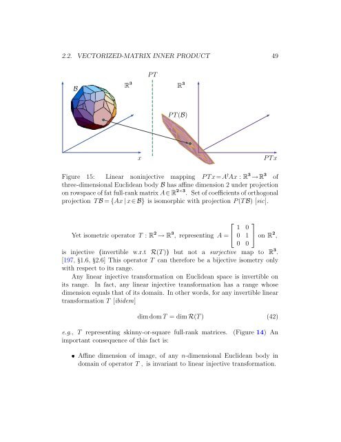
2.2. VECTORIZED-MATRIX INNER PRODUCT 49
B
R 3
PT
R 3
PT(B)
x
PTx
Figure 15: Linear noninjective mapping PTx=A † Ax : R 3 →R 3 of
three-dimensional Euclidean body B has affine dimension 2 under projection
on rowspace of fat full-rank matrix A∈ R 2×3 . Set of coefficients of orthogonal
projection T B = {Ax |x∈ B} is isomorphic with projection P(T B) [sic].
Yet isometric operator T : R 2 → R 3 , representing A = ⎣
⎡
1 0
0 1
0 0
⎤
⎦ on R 2 ,
is injective (invertible w.r.t R(T)) but not a surjective map to R 3 .
[197,1.6,2.6] This operator T can therefore be a bijective isometry only
with respect to its range.
Any linear injective transformation on Euclidean space is invertible on
its range. In fact, any linear injective transformation has a range whose
dimension equals that of its domain. In other words, for any invertible linear
transformation T [ibidem]
dim domT = dim R(T) (42)
e.g., T representing skinny-or-square full-rank matrices. (Figure 14) An
important consequence of this fact is:
Affine dimension of image, of any n-dimensional Euclidean body in
domain of operator T , is invariant to linear injective transformation.