v2009.01.01 - Convex Optimization
v2009.01.01 - Convex Optimization v2009.01.01 - Convex Optimization
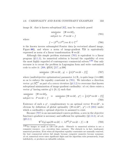
332 CHAPTER 4. SEMIDEFINITE PROGRAMMING vec −1 f Figure 88: Aliasing of Shepp-Logan phantom in Figure 86 resulting from k-space subsampling pattern in Figure 87. This image is real because binary mask Φ is vertically and horizontally symmetric. It is remarkable that the phantom can be reconstructed, by convex iteration, given only U 0 = vec −1 f . Express an image-gradient estimate ⎡ U ∆ ∇U = ∆ ⎢ U ∆ T ⎣ ∆ U ∆ T U ⎤ ⎥ ⎦ ∈ R4n×n (763) that is a simple first-order difference of neighboring pixels (Figure 89) to the right, left, above, and below. 4.49 ByA.1.1 no.25, its vectorization: for Ψ i ∈ R n2 ×n 2 vec ∇U = ⎡ ⎢ ⎣ ⎤ ∆ T ⊗ I ∆ ⊗ I I ⊗ ∆ I ⊗ ∆ T ⎥ ⎦ vec U ∆ = ⎡ ⎢ ⎣ Ψ 1 Ψ T 1 Ψ 2 Ψ T 2 ⎤ ⎥ ⎦ vec U ∆ = Ψ vec U ∈ R 4n2 (764) where Ψ∈ R 4n2 ×n 2 . A total-variation minimization for reconstructing MRI 4.49 There is significant improvement in reconstruction quality by augmentation of a normally two-dimensional image-gradient to a four-dimensional estimate per pixel by inclusion of two polar directions. We find small improvement on real-life images, ≈1dB empirically, by further augmentation with diagonally adjacent pixel differences.
4.6. CARDINALITY AND RANK CONSTRAINT EXAMPLES 333 image U , that is known suboptimal [62], may be concisely posed where minimize ‖Ψ vec U‖ 1 U subject to P vec U = f (765) f = (F H ⊗F H ) vec K ∈ C n2 (766) is the known inverse subsampled Fourier data (a vectorized aliased image, Figure 88), and where a norm of image-gradient ∇U is equivalently expressed as norm of a linear transformation Ψ vec U . Although this simple problem statement (765) is equivalent to a linear program (3.1.3), its numerical solution is beyond the capability of even the most highly regarded of contemporary commercial solvers. 4.50 Our only recourse is to recast the problem in Lagrangian form and write customized code to solve it: [308,IIIA] [217, p.398] minimize 〈|Ψ vec U| , y〉 + 1λ‖P vec U − U 2 f‖2 2 (767) where (multiobjective optimization) parameter λ∈ R + is quite large (λ≈1E8) so as to enforce the equality constraint in (765). We introduce a direction vector y ∈ R 4n2 + as part of a convex iteration (4.5.2) to overcome that known suboptimal minimization of image-gradient cardinality: id est, there exists a vector y ⋆ having entries yi ⋆ ∈ {0, 1} such that minimize ‖Ψ vec U‖ 0 U subject to P vec U = f ≡ minimize U 〈|Ψ vec U| , y ⋆ 〉 + 1 2 λ‖P vec U − f‖2 2 (768) Existence of such a y ⋆ , complementary to an optimal vector Ψ vec U ⋆ , is obvious by definition of global optimality 〈|Ψ vec U ⋆ | , y ⋆ 〉= 0 (683) under which a cardinality-c optimal objective is assumed to exist. Because (767) is an unconstrained convex problem, a zero in the objective function’s gradient is necessary and sufficient for optimality (2.13.3); id est, (D.2.1) Ψ T δ(y) sgn(Ψ vec U) + λP H (P vec U − f) = 0 (769) 4.50 for images as small as 128×128 pixels. Obstacle to numerical solution is not a computer resource: e.g., execution time, memory. The obstacle is, in fact, inadequate numerical precision. Even when all dependent equality constraints are manually removed, the best commercial solvers fail simply because computer numerics become nonsense; id est, numerical errors enter significant digits and the algorithm exits prematurely, loops indefinitely, or produces an infeasible solution.
- Page 281 and 282: 4.4. RANK-CONSTRAINED SEMIDEFINITE
- Page 283 and 284: 4.4. RANK-CONSTRAINED SEMIDEFINITE
- Page 285 and 286: 4.4. RANK-CONSTRAINED SEMIDEFINITE
- Page 287 and 288: 4.4. RANK-CONSTRAINED SEMIDEFINITE
- Page 289 and 290: 4.4. RANK-CONSTRAINED SEMIDEFINITE
- Page 291 and 292: 4.4. RANK-CONSTRAINED SEMIDEFINITE
- Page 293 and 294: 4.4. RANK-CONSTRAINED SEMIDEFINITE
- Page 295 and 296: 4.5. CONSTRAINING CARDINALITY 295 m
- Page 297 and 298: 4.5. CONSTRAINING CARDINALITY 297 m
- Page 299 and 300: 4.5. CONSTRAINING CARDINALITY 299 a
- Page 301 and 302: 4.5. CONSTRAINING CARDINALITY 301 f
- Page 303 and 304: 4.5. CONSTRAINING CARDINALITY 303 n
- Page 305 and 306: 4.5. CONSTRAINING CARDINALITY 305 W
- Page 307 and 308: 4.5. CONSTRAINING CARDINALITY 307 t
- Page 309 and 310: 4.6. CARDINALITY AND RANK CONSTRAIN
- Page 311 and 312: 4.6. CARDINALITY AND RANK CONSTRAIN
- Page 313 and 314: 4.6. CARDINALITY AND RANK CONSTRAIN
- Page 315 and 316: 4.6. CARDINALITY AND RANK CONSTRAIN
- Page 317 and 318: 4.6. CARDINALITY AND RANK CONSTRAIN
- Page 319 and 320: 4.6. CARDINALITY AND RANK CONSTRAIN
- Page 321 and 322: 4.6. CARDINALITY AND RANK CONSTRAIN
- Page 323 and 324: 4.6. CARDINALITY AND RANK CONSTRAIN
- Page 325 and 326: 4.6. CARDINALITY AND RANK CONSTRAIN
- Page 327 and 328: 4.6. CARDINALITY AND RANK CONSTRAIN
- Page 329 and 330: 4.6. CARDINALITY AND RANK CONSTRAIN
- Page 331: 4.6. CARDINALITY AND RANK CONSTRAIN
- Page 335 and 336: 4.6. CARDINALITY AND RANK CONSTRAIN
- Page 337 and 338: 4.6. CARDINALITY AND RANK CONSTRAIN
- Page 339 and 340: 4.6. CARDINALITY AND RANK CONSTRAIN
- Page 341 and 342: 4.7. CONVEX ITERATION RANK-1 341 fi
- Page 343 and 344: 4.7. CONVEX ITERATION RANK-1 343 Gi
- Page 345 and 346: Chapter 5 Euclidean Distance Matrix
- Page 347 and 348: 5.2. FIRST METRIC PROPERTIES 347 co
- Page 349 and 350: 5.3. ∃ FIFTH EUCLIDEAN METRIC PRO
- Page 351 and 352: 5.3. ∃ FIFTH EUCLIDEAN METRIC PRO
- Page 353 and 354: 5.4. EDM DEFINITION 353 The collect
- Page 355 and 356: 5.4. EDM DEFINITION 355 5.4.2 Gram-
- Page 357 and 358: 5.4. EDM DEFINITION 357 D ∈ EDM N
- Page 359 and 360: 5.4. EDM DEFINITION 359 5.4.2.2.1 E
- Page 361 and 362: 5.4. EDM DEFINITION 361 ten affine
- Page 363 and 364: 5.4. EDM DEFINITION 363 spheres: Th
- Page 365 and 366: 5.4. EDM DEFINITION 365 By eliminat
- Page 367 and 368: 5.4. EDM DEFINITION 367 where Φ ij
- Page 369 and 370: 5.4. EDM DEFINITION 369 5.4.2.2.6 D
- Page 371 and 372: 5.4. EDM DEFINITION 371 10 5 ˇx 4
- Page 373 and 374: 5.4. EDM DEFINITION 373 corrected b
- Page 375 and 376: 5.4. EDM DEFINITION 375 by translat
- Page 377 and 378: 5.4. EDM DEFINITION 377 Crippen & H
- Page 379 and 380: 5.4. EDM DEFINITION 379 where ([√
- Page 381 and 382: 5.4. EDM DEFINITION 381 because (A.
4.6. CARDINALITY AND RANK CONSTRAINT EXAMPLES 333<br />
image U , that is known suboptimal [62], may be concisely posed<br />
where<br />
minimize ‖Ψ vec U‖ 1<br />
U<br />
subject to P vec U = f<br />
(765)<br />
f = (F H ⊗F H ) vec K ∈ C n2 (766)<br />
is the known inverse subsampled Fourier data (a vectorized aliased image,<br />
Figure 88), and where a norm of image-gradient ∇U is equivalently<br />
expressed as norm of a linear transformation Ψ vec U .<br />
Although this simple problem statement (765) is equivalent to a linear<br />
program (3.1.3), its numerical solution is beyond the capability of even<br />
the most highly regarded of contemporary commercial solvers. 4.50 Our only<br />
recourse is to recast the problem in Lagrangian form and write customized<br />
code to solve it: [308,IIIA] [217, p.398]<br />
minimize 〈|Ψ vec U| , y〉 + 1λ‖P vec U −<br />
U<br />
2 f‖2 2 (767)<br />
where (multiobjective optimization) parameter λ∈ R + is quite large (λ≈1E8)<br />
so as to enforce the equality constraint in (765). We introduce a direction<br />
vector y ∈ R 4n2<br />
+ as part of a convex iteration (4.5.2) to overcome that known<br />
suboptimal minimization of image-gradient cardinality: id est, there exists a<br />
vector y ⋆ having entries yi ⋆ ∈ {0, 1} such that<br />
minimize ‖Ψ vec U‖ 0<br />
U<br />
subject to P vec U = f<br />
≡<br />
minimize<br />
U<br />
〈|Ψ vec U| , y ⋆ 〉 + 1 2 λ‖P vec U − f‖2 2<br />
(768)<br />
Existence of such a y ⋆ , complementary to an optimal vector Ψ vec U ⋆ , is<br />
obvious by definition of global optimality 〈|Ψ vec U ⋆ | , y ⋆ 〉= 0 (683) under<br />
which a cardinality-c optimal objective is assumed to exist.<br />
Because (767) is an unconstrained convex problem, a zero in the objective<br />
function’s gradient is necessary and sufficient for optimality (2.13.3); id est,<br />
(D.2.1)<br />
Ψ T δ(y) sgn(Ψ vec U) + λP H (P vec U − f) = 0 (769)<br />
4.50 for images as small as 128×128 pixels. Obstacle to numerical solution is not a<br />
computer resource: e.g., execution time, memory. The obstacle is, in fact, inadequate<br />
numerical precision. Even when all dependent equality constraints are manually removed,<br />
the best commercial solvers fail simply because computer numerics become nonsense;<br />
id est, numerical errors enter significant digits and the algorithm exits prematurely, loops<br />
indefinitely, or produces an infeasible solution.


