A. Linear Algebra - Meboo Publishing featured book, Convex ...

Appendix A
Linear algebra
A.1 Main-diagonal δ operator, λ , trace, vec
We introduce notation δ denoting the main-diagonal linear self-adjoint
operator. When linear function δ operates on a square matrix A∈ R N×N ,
δ(A) returns a vector composed of all the entries from the main diagonal in
the natural order;
δ(A) ∈ R N (1391)
Operating on a vector y ∈ R N , δ naturally returns a diagonal matrix;
δ(y) ∈ S N (1392)
Operating recursively on a vector Λ∈ R N or diagonal matrix Λ∈ S N ,
δ(δ(Λ)) returns Λ itself;
δ 2 (Λ) ≡ δ(δ(Λ)) Λ (1393)
Defined in this manner, main-diagonal linear operator δ is self-adjoint
[222,3.10,9.5-1]; A.1 videlicet, (2.2)
δ(A) T y = 〈δ(A), y〉 = 〈A , δ(y)〉 = tr ( A T δ(y) ) (1394)
A.1 Linear operator T : R m×n → R M×N is self-adjoint when, for each and every
X 1 , X 2 ∈ R m×n 〈T(X 1 ), X 2 〉 = 〈X 1 , T(X 2 )〉
2001 Jon Dattorro. co&edg version 2010.01.05. All rights reserved.
citation: Dattorro, Convex Optimization & Euclidean Distance Geometry,
Mεβoo Publishing USA, 2005, v2010.01.05.
581

582 APPENDIX A. LINEAR ALGEBRA
A.1.1
Identities
This δ notation is efficient and unambiguous as illustrated in the following
examples where: A ◦ B denotes Hadamard product [198] [155,1.1.4] of
matrices of like size, ⊗ Kronecker product [162] (D.1.2.1), y a vector, X
a matrix, e i the i th member of the standard basis for R n , S N h the symmetric
hollow subspace, σ(A) a vector of (nonincreasingly) ordered singular values,
and λ(A) a vector of nonincreasingly ordered eigenvalues of matrix A :
1. δ(A) = δ(A T )
2. tr(A) = tr(A T ) = δ(A) T 1 = 〈I, A〉
3. δ(cA) = cδ(A) c∈R
4. tr(cA) = c tr(A) = c1 T λ(A) c∈R
5. vec(cA) = c vec(A) c∈R
6. A ◦ cB = cA ◦ B c∈R
7. A ⊗ cB = cA ⊗ B c∈R
8. δ(A + B) = δ(A) + δ(B)
9. tr(A + B) = tr(A) + tr(B)
10. vec(A + B) = vec(A) + vec(B)
11. (A + B) ◦ C = A ◦ C + B ◦ C
A ◦ (B + C) = A ◦ B + A ◦ C
12. (A + B) ⊗ C = A ⊗ C + B ⊗ C
A ⊗ (B + C) = A ⊗ B + A ⊗ C
13. sgn(c)λ(|c|A) = cλ(A) c∈R
14. sgn(c)σ(|c|A) = cσ(A) c∈R
15. tr(c √ A T A) = c tr √ A T A = c1 T σ(A) c∈R
16. π(δ(A)) = λ(I ◦A) where π is the presorting function.
17. δ(AB) = (A ◦ B T )1 = (B T ◦ A)1
18. δ(AB) T = 1 T (A T ◦ B) = 1 T (B ◦ A T )

A.1. MAIN-DIAGONAL δ OPERATOR, λ , TRACE, VEC 583
⎡ ⎤
u 1 v 1
19. δ(uv T ⎢ ⎥
) = ⎣ . ⎦ = u ◦ v ,
u N v N
u,v ∈ R N
20. tr(A T B) = tr(AB T ) = tr(BA T ) = tr(B T A)
= 1 T (A ◦ B)1 = 1 T δ(AB T ) = δ(A T B) T 1 = δ(BA T ) T 1 = δ(B T A) T 1
21. D = [d ij ] ∈ S N h , H = [h ij ] ∈ S N h , V = I − 1 N 11T ∈ S N (conferB.4.2 no.20)
N tr(−V (D ◦ H)V ) = tr(D T H) = 1 T (D ◦ H)1 = tr(11 T (D ◦ H)) = ∑ d ij h ij
i,j
22. tr(ΛA) = δ(Λ) T δ(A), δ 2 (Λ) Λ ∈ S N
23. y T Bδ(A) = tr ( Bδ(A)y T) = tr ( δ(B T y)A ) = tr ( Aδ(B T y) )
= δ(A) T B T y = tr ( yδ(A) T B T) = tr ( A T δ(B T y) ) = tr ( δ(B T y)A T)
24. δ 2 (A T A) = ∑ i
e i e T iA T Ae i e T i
25. δ ( δ(A)1 T) = δ ( 1δ(A) T) = δ(A)
26. δ(A1)1 = δ(A11 T ) = A1 , δ(y)1 = δ(y1 T ) = y
27. δ(I1) = δ(1) = I
28. δ(e i e T j 1) = δ(e i ) = e i e T i
29. For ζ =[ζ i ]∈ R k and x=[x i ]∈ R k ,
30.
∑
ζ i /x i = ζ T δ(x) −1 1
vec(A ◦ B) = vec(A) ◦ vec(B) = δ(vecA) vec(B)
= vec(B) ◦ vec(A) = δ(vecB) vec(A)
31. vec(AXB) = (B T ⊗ A) vec X
32. vec(BXA) = (A T ⊗ B) vec X
i
(42)(1747)
(
not
H )
33.
34.
tr(AXBX T ) = vec(X) T vec(AXB) = vec(X) T (B T ⊗ A) vec X [162]
= δ ( vec(X) vec(X) T (B T ⊗ A) ) T
1
tr(AX T BX) = vec(X) T vec(BXA) = vec(X) T (A T ⊗ B) vec X
= δ ( vec(X) vec(X) T (A T ⊗ B) ) T
1

584 APPENDIX A. LINEAR ALGEBRA
35. For any permutation matrix Ξ and dimensionally compatible vector y
or matrix A
δ(Ξy) = Ξδ(y) Ξ T (1395)
δ(ΞAΞ T ) = Ξδ(A) (1396)
So given any permutation matrix Ξ and any dimensionally compatible
matrix B , for example,
δ 2 (B) = Ξδ 2 (Ξ T B Ξ)Ξ T (1397)
36. A ⊗ 1 = 1 ⊗ A = A
37. A ⊗ (B ⊗ C) = (A ⊗ B) ⊗ C
38. (A ⊗ B)(C ⊗ D) = AC ⊗ BD
39. For A a vector, (A ⊗ B) = (A ⊗ I)B
40. For B a row vector, (A ⊗ B) = A(I ⊗ B)
41. (A ⊗ B) T = A T ⊗ B T
42. (A ⊗ B) −1 = A −1 ⊗ B −1
43. tr(A ⊗ B) = trA trB
44. For A∈ R m×m , B ∈ R n×n , det(A ⊗ B) = det n (A) det m (B)
45. There exist permutation matrices Ξ 1 and Ξ 2 such that [162, p.28]
A ⊗ B = Ξ 1 (B ⊗ A)Ξ 2 (1398)
46. For eigenvalues λ(A)∈ C n and eigenvectors v(A)∈ C n×n such that
A = vδ(λ)v −1 ∈ R n×n
λ(A ⊗ B) = λ(A) ⊗ λ(B) , v(A ⊗ B) = v(A) ⊗ v(B) (1399)
47. Given analytic function [80] f : C n×n → C n×n , then f(I ⊗A)= I ⊗f(A)
and f(A ⊗ I) = f(A) ⊗ I [162, p.28]

A.1. MAIN-DIAGONAL δ OPERATOR, λ , TRACE, VEC 585
A.1.2
Majorization
A.1.2.0.1 Theorem. (Schur) Majorization. [386,7.4] [198,4.3]
[199,5.5] Let λ∈ R N denote a given vector of eigenvalues and let
δ ∈ R N denote a given vector of main diagonal entries, both arranged in
nonincreasing order. Then
and conversely
∃A∈ S N λ(A)=λ and δ(A)= δ ⇐ λ − δ ∈ K ∗ λδ (1400)
A∈ S N ⇒ λ(A) − δ(A) ∈ K ∗ λδ (1401)
The difference belongs to the pointed polyhedral cone of majorization (empty
interior, confer (291))
K ∗ λδ K ∗ M+ ∩ {ζ1 | ζ ∈ R} ∗ (1402)
where K ∗ M+ is the dual monotone nonnegative cone (413), and where the
dual of the line is a hyperplane; ∂H = {ζ1 | ζ ∈ R} ∗ = 1 ⊥ .
⋄
Majorization cone K ∗ λδ is naturally consequent to the definition of
majorization; id est, vector y ∈ R N majorizes vector x if and only if
k∑
x i ≤
i=1
k∑
y i ∀ 1 ≤ k ≤ N (1403)
i=1
and
1 T x = 1 T y (1404)
Under these circumstances, rather, vector x is majorized by vector y .
In the particular circumstance δ(A)=0 we get:
A.1.2.0.2 Corollary. Symmetric hollow majorization.
Let λ∈ R N denote a given vector of eigenvalues arranged in nonincreasing
order. Then
∃A∈ S N h λ(A)=λ ⇐ λ ∈ K ∗ λδ (1405)
and conversely
where K ∗ λδ
is defined in (1402).
⋄
A∈ S N h ⇒ λ(A) ∈ K ∗ λδ (1406)

586 APPENDIX A. LINEAR ALGEBRA
A.2 Semidefiniteness: domain of test
The most fundamental necessary, sufficient, and definitive test for positive
semidefiniteness of matrix A ∈ R n×n is: [199,1]
x T Ax ≥ 0 for each and every x ∈ R n such that ‖x‖ = 1 (1407)
Traditionally, authors demand evaluation over broader domain; namely,
over all x ∈ R n which is sufficient but unnecessary. Indeed, that standard
textbook requirement is far over-reaching because if x T Ax is nonnegative for
particular x = x p , then it is nonnegative for any αx p where α∈ R . Thus,
only normalized x in R n need be evaluated.
Many authors add the further requirement that the domain be complex;
the broadest domain. By so doing, only Hermitian matrices (A H = A where
superscript H denotes conjugate transpose) A.2 are admitted to the set of
positive semidefinite matrices (1410); an unnecessary prohibitive condition.
A.2.1
Symmetry versus semidefiniteness
We call (1407) the most fundamental test of positive semidefiniteness. Yet
some authors instead say, for real A and complex domain {x∈ C n } , the
complex test x H Ax≥0 is most fundamental. That complex broadening of the
domain of test causes nonsymmetric real matrices to be excluded from the set
of positive semidefinite matrices. Yet admitting nonsymmetric real matrices
or not is a matter of preference A.3 unless that complex test is adopted, as we
shall now explain.
Any real square matrix A has a representation in terms of its symmetric
and antisymmetric parts; id est,
A = (A +AT )
2
+ (A −AT )
2
(53)
Because, for all real A , the antisymmetric part vanishes under real test,
x T(A −AT )
2
x = 0 (1408)
A.2 Hermitian symmetry is the complex analogue; the real part of a Hermitian matrix
is symmetric while its imaginary part is antisymmetric. A Hermitian matrix has real
eigenvalues and real main diagonal.
A.3 Golub & Van Loan [155,4.2.2], for example, admit nonsymmetric real matrices.

A.2. SEMIDEFINITENESS: DOMAIN OF TEST 587
only the symmetric part of A , (A +A T )/2, has a role determining positive
semidefiniteness. Hence the oft-made presumption that only symmetric
matrices may be positive semidefinite is, of course, erroneous under (1407).
Because eigenvalue-signs of a symmetric matrix translate unequivocally to
its semidefiniteness, the eigenvalues that determine semidefiniteness are
always those of the symmetrized matrix. (A.3) For that reason, and
because symmetric (or Hermitian) matrices must have real eigenvalues,
the convention adopted in the literature is that semidefinite matrices are
synonymous with symmetric semidefinite matrices. Certainly misleading
under (1407), that presumption is typically bolstered with compelling
examples from the physical sciences where symmetric matrices occur within
the mathematical exposition of natural phenomena. A.4 [137,52]
Perhaps a better explanation of this pervasive presumption of symmetry
comes from Horn & Johnson [198,7.1] whose perspective A.5 is the complex
matrix, thus necessitating the complex domain of test throughout their
treatise. They explain, if A∈C n×n
...and if x H Ax is real for all x ∈ C n , then A is Hermitian.
Thus, the assumption that A is Hermitian is not necessary in the
definition of positive definiteness. It is customary, however.
Their comment is best explained by noting, the real part of x H Ax comes
from the Hermitian part (A +A H )/2 of A ;
rather,
re(x H Ax) = x
HA +AH
x (1409)
2
x H Ax ∈ R ⇔ A H = A (1410)
because the imaginary part of x H Ax comes from the anti-Hermitian part
(A −A H )/2 ;
im(x H Ax) = x
HA −AH
x (1411)
2
that vanishes for nonzero x if and only if A = A H . So the Hermitian
symmetry assumption is unnecessary, according to Horn & Johnson, not
A.4 Symmetric matrices are certainly pervasive in the our chosen subject as well.
A.5 A totally complex perspective is not necessarily more advantageous. The positive
semidefinite cone, for example, is not selfdual (2.13.5) in the ambient space of Hermitian
matrices. [192,II]

588 APPENDIX A. LINEAR ALGEBRA
because nonHermitian matrices could be regarded positive semidefinite,
rather because nonHermitian (includes nonsymmetric real) matrices are not
comparable on the real line under x H Ax . Yet that complex edifice is
dismantled in the test of real matrices (1407) because the domain of test
is no longer necessarily complex; meaning, x T Ax will certainly always be
real, regardless of symmetry, and so real A will always be comparable.
In summary, if we limit the domain of test to all x in R n as in (1407),
then nonsymmetric real matrices are admitted to the realm of semidefinite
matrices because they become comparable on the real line. One important
exception occurs for rank-one matrices Ψ=uv T where u and v are real
vectors: Ψ is positive semidefinite if and only if Ψ=uu T . (A.3.1.0.7)
We might choose to expand the domain of test to all x in C n so that only
symmetric matrices would be comparable. The alternative to expanding
domain of test is to assume all matrices of interest to be symmetric; that
is commonly done, hence the synonymous relationship with semidefinite
matrices.
A.2.1.0.1 Example. Nonsymmetric positive definite product.
Horn & Johnson assert and Zhang agrees:
If A,B ∈ C n×n are positive definite, then we know that the
product AB is positive definite if and only if AB is Hermitian.
[198,7.6, prob.10] [386,6.2,3.2]
Implicitly in their statement, A and B are assumed individually Hermitian
and the domain of test is assumed complex.
We prove that assertion to be false for real matrices under (1407) that
adopts a real domain of test.
A T = A =
⎡
⎢
⎣
3 0 −1 0
0 5 1 0
−1 1 4 1
0 0 1 4
⎤
⎥
⎦ ,
⎡
λ(A) = ⎢
⎣
5.9
4.5
3.4
2.0
⎤
⎥
⎦ (1412)
B T = B =
⎡
⎢
⎣
4 4 −1 −1
4 5 0 0
−1 0 5 1
−1 0 1 4
⎤
⎥
⎦ ,
⎡
λ(B) = ⎢
⎣
8.8
5.5
3.3
0.24
⎤
⎥
⎦ (1413)

A.3. PROPER STATEMENTS 589
(AB) T ≠ AB =
⎡
⎢
⎣
13 12 −8 −4
19 25 5 1
−5 1 22 9
−5 0 9 17
⎤
⎥
⎦ ,
⎡
λ(AB) = ⎢
⎣
36.
29.
10.
0.72
⎤
⎥
⎦ (1414)
1
(AB + 2 (AB)T ) =
⎡
⎢
⎣
13 15.5 −6.5 −4.5
15.5 25 3 0.5
−6.5 3 22 9
−4.5 0.5 9 17
⎤
⎥
⎦ , λ( 1
2 (AB + (AB)T ) ) =
⎡
⎢
⎣
36.
30.
10.
0.014
(1415)
Whenever A∈ S n + and B ∈ S n + , then λ(AB)=λ( √ AB √ A) will always
be a nonnegative vector by (1439) and Corollary A.3.1.0.5. Yet positive
definiteness of product AB is certified instead by the nonnegative eigenvalues
λ ( 1
2 (AB + (AB)T ) ) in (1415) (A.3.1.0.1) despite the fact that AB is not
symmetric. A.6 Horn & Johnson and Zhang resolve the anomaly by choosing
to exclude nonsymmetric matrices and products; they do so by expanding
the domain of test to C n .
⎤
⎥
⎦
A.3 Proper statements
of positive semidefiniteness
Unlike Horn & Johnson and Zhang, we never adopt a complex domain of test
with real matrices. So motivated is our consideration of proper statements
of positive semidefiniteness under real domain of test. This restriction,
ironically, complicates the facts when compared to corresponding statements
for the complex case (found elsewhere [198] [386]).
We state several fundamental facts regarding positive semidefiniteness of
real matrix A and the product AB and sum A +B of real matrices under
fundamental real test (1407); a few require proof as they depart from the
standard texts, while those remaining are well established or obvious.
A.6 It is a little more difficult to find a counter-example in R 2×2 or R 3×3 ; which may
have served to advance any confusion.

590 APPENDIX A. LINEAR ALGEBRA
A.3.0.0.1 Theorem. Positive (semi)definite matrix.
A∈ S M is positive semidefinite if and only if for each and every vector x∈ R M
of unit norm, ‖x‖ = 1 , A.7 we have x T Ax ≥ 0 (1407);
A ≽ 0 ⇔ tr(xx T A) = x T Ax ≥ 0 ∀xx T (1416)
Matrix A ∈ S M is positive definite if and only if for each and every ‖x‖ = 1
we have x T Ax > 0 ;
A ≻ 0 ⇔ tr(xx T A) = x T Ax > 0 ∀xx T , xx T ≠ 0 (1417)
Proof. Statements (1416) and (1417) are each a particular instance
of dual generalized inequalities (2.13.2) with respect to the positive
semidefinite cone; videlicet, [353]
⋄
A ≽ 0 ⇔ 〈xx T , A〉 ≥ 0 ∀xx T (≽ 0)
A ≻ 0 ⇔ 〈xx T , A〉 > 0 ∀xx T (≽ 0), xx T ≠ 0
(1418)
This says: positive semidefinite matrix A must belong to the normal side
of every hyperplane whose normal is an extreme direction of the positive
semidefinite cone. Relations (1416) and (1417) remain true when xx T is
replaced with “for each and every” positive semidefinite matrix X ∈ S M +
(2.13.5) of unit norm, ‖X‖= 1, as in
A ≽ 0 ⇔ tr(XA) ≥ 0 ∀X ∈ S M +
A ≻ 0 ⇔ tr(XA) > 0 ∀X ∈ S M + , X ≠ 0
(1419)
But that condition is more than what is necessary. By the discretized
membership theorem in2.13.4.2.1, the extreme directions xx T of the positive
semidefinite cone constitute a minimal set of generators necessary and
sufficient for discretization of dual generalized inequalities (1419) certifying
membership to that cone.
A.7 The traditional condition requiring all x∈ R M for defining positive (semi)definiteness
is actually more than what is necessary. The set of norm-1 vectors is necessary and
sufficient to establish positive semidefiniteness; actually, any particular norm and any
nonzero norm-constant will work.

A.3. PROPER STATEMENTS 591
A.3.1
Semidefiniteness, eigenvalues, nonsymmetric
When A∈ R n×n , let λ ( 1
2 (A +AT ) ) ∈ R n denote eigenvalues of the
symmetrized matrix A.8 arranged in nonincreasing order.
By positive semidefiniteness of A∈ R n×n we mean, A.9 [266,1.3.1]
(conferA.3.1.0.1)
x T Ax ≥ 0 ∀x∈ R n ⇔ A +A T ≽ 0 ⇔ λ(A +A T ) ≽ 0 (1420)
(2.9.0.1)
A ≽ 0 ⇒ A T = A (1421)
A ≽ B ⇔ A −B ≽ 0 A ≽ 0 or B ≽ 0 (1422)
x T Ax≥0 ∀x A T = A (1423)
Matrix symmetry is not intrinsic to positive semidefiniteness;
A T = A, λ(A) ≽ 0 ⇒ x T Ax ≥ 0 ∀x (1424)
If A T = A thenλ(A) ≽ 0 ⇐ A T = A, x T Ax ≥ 0 ∀x (1425)
λ(A) ≽ 0 ⇔ A ≽ 0 (1426)
meaning, matrix A belongs to the positive semidefinite cone in the
subspace of symmetric matrices if and only if its eigenvalues belong to
the nonnegative orthant.
〈A , A〉 = 〈λ(A), λ(A)〉 (45)
For µ∈ R , A∈ R n×n , and vector λ(A)∈ C n holding the ordered
eigenvalues of A
λ(µI + A) = µ1 + λ(A) (1427)
Proof: A=MJM −1 and µI + A = M(µI + J)M −1 where J
is the Jordan form for A ; [325,5.6, App.B] id est, δ(J) = λ(A) ,
so λ(µI + A) = δ(µI + J) because µI + J is also a Jordan form.
A.8 The symmetrization of A is (A +A T )/2. λ ( 1
2 (A +AT ) ) = λ(A +A T )/2.
A.9 Strang agrees [325, p.334] it is not λ(A) that requires observation. Yet he is mistaken
by proposing the Hermitian part alone x H (A+A H )x be tested, because the anti-Hermitian
part does not vanish under complex test unless A is Hermitian. (1411)

592 APPENDIX A. LINEAR ALGEBRA
By similar reasoning,
λ(I + µA) = 1 + λ(µA) (1428)
For vector σ(A) holding the singular values of any matrix A
σ(I + µA T A) = π(|1 + µσ(A T A)|) (1429)
σ(µI + A T A) = π(|µ1 + σ(A T A)|) (1430)
where π is the nonlinear permutation-operator sorting its vector
argument into nonincreasing order.
For A∈ S M and each and every ‖w‖= 1 [198,7.7, prob.9]
w T Aw ≤ µ ⇔ A ≼ µI ⇔ λ(A) ≼ µ1 (1431)
[198,2.5.4] (confer (44))
A is normal matrix ⇔ ‖A‖ 2 F = λ(A) T λ(A) (1432)
For A∈ R m×n A T A ≽ 0, AA T ≽ 0 (1433)
because, for dimensionally compatible vector x , x T A T Ax = ‖Ax‖ 2 2 ,
x T AA T x = ‖A T x‖ 2 2 .
For A∈ R n×n and c∈R
tr(cA) = c tr(A) = c1 T λ(A)
(A.1.1 no.4)
For m a nonnegative integer, (1828)
det(A m ) =
tr(A m ) =
n∏
λ(A) m i (1434)
i=1
n∑
λ(A) m i (1435)
i=1

A.3. PROPER STATEMENTS 593
For A diagonalizable (A.5), A = SΛS −1 , (confer [325, p.255])
rankA = rankδ(λ(A)) = rank Λ (1436)
meaning, rank is equal to the number of nonzero eigenvalues in vector
by the 0 eigenvalues theorem (A.7.3.0.1).
(Ky Fan) For A,B∈ S n [53,1.2] (confer (1703))
λ(A) δ(Λ) (1437)
tr(AB) ≤ λ(A) T λ(B) (1689)
with equality (Theobald) when A and B are simultaneously
diagonalizable [198] with the same ordering of eigenvalues.
For A∈ R m×n and B ∈ R n×m
tr(AB) = tr(BA) (1438)
and η eigenvalues of the product and commuted product are identical,
including their multiplicity; [198,1.3.20] id est,
λ(AB) 1:η = λ(BA) 1:η , ηmin{m , n} (1439)
Any eigenvalues remaining are zero. By the 0 eigenvalues theorem
(A.7.3.0.1),
rank(AB) = rank(BA), AB and BA diagonalizable (1440)
For any compatible matrices A,B [198,0.4]
min{rankA, rankB} ≥ rank(AB) (1441)
For A,B ∈ S n +
rankA + rankB ≥ rank(A + B) ≥ min{rankA, rankB} ≥ rank(AB)
(1442)
For linearly independent matrices A,B ∈ S n + (2.1.2, R(A) ∩ R(B)=0,
R(A T ) ∩ R(B T )=0,B.1.1),
rankA + rankB = rank(A + B) > min{rankA, rankB} ≥ rank(AB)
(1443)

594 APPENDIX A. LINEAR ALGEBRA
Because R(A T A)= R(A T ) and R(AA T )= R(A) (p.624), for any
A∈ R m×n rank(AA T ) = rank(A T A) = rankA = rankA T (1444)
For A∈ R m×n having no nullspace, and for any B ∈ R n×k
rank(AB) = rank(B) (1445)
Proof. For any compatible matrix C , N(CAB)⊇ N(AB)⊇ N(B)
is obvious. By assumption ∃A † A † A = I . Let C = A † , then
N(AB)= N(B) and the stated result follows by conservation of
dimension (1549).
For A∈ S n and any nonsingular matrix Y
inertia(A) = inertia(YAY T ) (1446)
a.k.a, Sylvester’s law of inertia. (1489) [110,2.4.3]
For A,B∈R n×n square, [198,0.3.5]
Yet for A∈ R m×n and B ∈ R n×m [75, p.72]
det(AB) = det(BA) (1447)
det(AB) = detA detB (1448)
det(I + AB) = det(I + BA) (1449)
For A,B ∈ S n , product AB is symmetric if and only if AB is
commutative;
(AB) T = AB ⇔ AB = BA (1450)
Proof. (⇒) Suppose AB=(AB) T . (AB) T =B T A T =BA .
AB=(AB) T ⇒ AB=BA .
(⇐) Suppose AB=BA . BA=B T A T =(AB) T . AB=BA ⇒
AB=(AB) T .
Commutativity alone is insufficient for symmetry of the product.
[325, p.26]

A.3. PROPER STATEMENTS 595
Diagonalizable matrices A,B∈R n×n commute if and only if they are
simultaneously diagonalizable. [198,1.3.12] A product of diagonal
matrices is always commutative.
For A,B ∈ R n×n and AB = BA
x T Ax ≥ 0, x T Bx ≥ 0 ∀x ⇒ λ(A+A T ) i λ(B+B T ) i ≥ 0 ∀i x T ABx ≥ 0 ∀x
(1451)
the negative result arising because of the schism between the product
of eigenvalues λ(A + A T ) i λ(B + B T ) i and the eigenvalues of the
symmetrized matrix product λ(AB + (AB) T ) i
. For example, X 2 is
generally not positive semidefinite unless matrix X is symmetric; then
(1433) applies. Simply substituting symmetric matrices changes the
outcome:
For A,B ∈ S n and AB = BA
A ≽ 0, B ≽ 0 ⇒ λ(AB) i =λ(A) i λ(B) i ≥0 ∀i ⇔ AB ≽ 0 (1452)
Positive semidefiniteness of A and B is sufficient but not a necessary
condition for positive semidefiniteness of the product AB .
Proof. Because all symmetric matrices are diagonalizable, (A.5.1)
[325,5.6] we have A=SΛS T and B=T∆T T , where Λ and ∆ are
real diagonal matrices while S and T are orthogonal matrices. Because
(AB) T =AB , then T must equal S , [198,1.3] and the eigenvalues of
A are ordered in the same way as those of B ; id est, λ(A) i =δ(Λ) i and
λ(B) i =δ(∆) i correspond to the same eigenvector.
(⇒) Assume λ(A) i λ(B) i ≥0 for i=1... n . AB=SΛ∆S T is
symmetric and has nonnegative eigenvalues contained in diagonal
matrix Λ∆ by assumption; hence positive semidefinite by (1420). Now
assume A,B ≽0. That, of course, implies λ(A) i λ(B) i ≥0 for all i
because all the individual eigenvalues are nonnegative.
(⇐) Suppose AB=SΛ∆S T ≽ 0. Then Λ∆≽0 by (1420),
and so all products λ(A) i λ(B) i must be nonnegative; meaning,
sgn(λ(A))= sgn(λ(B)). We may, therefore, conclude nothing about
the semidefiniteness of A and B .

596 APPENDIX A. LINEAR ALGEBRA
For A,B ∈ S n and A ≽ 0, B ≽ 0 (Example A.2.1.0.1)
AB = BA ⇒ λ(AB) i =λ(A) i λ(B) i ≥ 0 ∀i ⇒ AB ≽ 0 (1453)
AB = BA ⇒ λ(AB) i ≥ 0, λ(A) i λ(B) i ≥ 0 ∀i ⇔ AB ≽ 0 (1454)
For A,B ∈ S n [199,4.2.13]
A ≽ 0, B ≽ 0 ⇒ A ⊗ B ≽ 0 (1455)
A ≻ 0, B ≻ 0 ⇒ A ⊗ B ≻ 0 (1456)
and the Kronecker product is symmetric.
For A,B ∈ S n [386,6.2]
A ≽ 0 ⇒ trA ≥ 0 (1457)
A ≽ 0, B ≽ 0 ⇒ trA trB ≥ tr(AB) ≥ 0 (1458)
Because A ≽ 0, B ≽ 0 ⇒ λ(AB) = λ( √ AB √ A) ≽ 0 by (1439) and
Corollary A.3.1.0.5, then we have tr(AB) ≥ 0.
A ≽ 0 ⇔ tr(AB)≥ 0 ∀B ≽ 0 (356)
For A,B,C ∈ S n (Löwner)
A ≼ B , B ≼ C ⇒ A ≼ C
A ≼ B ⇔ A + C ≼ B + C
A ≼ B , A ≽ B ⇒ A = B
A ≼ A
A ≼ B , B ≺ C ⇒ A ≺ C
A ≺ B ⇔ A + C ≺ B + C
(transitivity)
(additivity)
(antisymmetry)
(reflexivity)
(strict transitivity)
(strict additivity)
(1459)
(1460)
For A,B ∈ R n×n x T Ax ≥ x T Bx ∀x ⇒ trA ≥ trB (1461)
Proof. x T Ax≥x T Bx ∀x ⇔ λ((A −B) + (A −B) T )/2 ≽ 0 ⇒
tr(A+A T −(B+B T ))/2 = tr(A −B)≥0. There is no converse.

A.3. PROPER STATEMENTS 597
For A,B ∈ S n [386,6.2] (Theorem A.3.1.0.4)
A ≽ B ⇒ trA ≥ trB (1462)
A ≽ B ⇒ δ(A) ≽ δ(B) (1463)
There is no converse, and restriction to the positive semidefinite cone
does not improve the situation. All-strict versions hold.
A ≽ B ≽ 0 ⇒ rankA ≥ rankB (1464)
A ≽ B ≽ 0 ⇒ detA ≥ detB ≥ 0 (1465)
A ≻ B ≽ 0 ⇒ detA > detB ≥ 0 (1466)
For A,B ∈ int S n + [33,4.2] [198,7.7.4]
A ≽ B ⇔ A −1 ≼ B −1 , A ≻ 0 ⇔ A −1 ≻ 0 (1467)
For A,B ∈ S n [386,6.2]
A ≽ B ≽ 0 ⇒ √ A ≽ √ B (1468)
For A,B ∈ S n and AB = BA [386,6.2, prob.3]
A ≽ B ≽ 0 ⇒ A k ≽ B k , k=1, 2,... (1469)
A.3.1.0.1 Theorem. Positive semidefinite ordering of eigenvalues.
For A,B∈ R M×M , place the eigenvalues of each symmetrized matrix into
the respective vectors λ ( 1
(A 2 +AT ) ) , λ ( 1
(B 2 +BT ) ) ∈ R M . Then, [325,6]
x T Ax ≥ 0 ∀x ⇔ λ ( A +A T) ≽ 0 (1470)
x T Ax > 0 ∀x ≠ 0 ⇔ λ ( A +A T) ≻ 0 (1471)
because x T (A −A T )x=0. (1408) Now arrange the entries of λ ( 1
(A 2 +AT ) )
and λ ( 1
(B 2 +BT ) ) in nonincreasing order so λ ( 1
(A 2 +AT ) ) holds the
1
largest eigenvalue of symmetrized A while λ ( 1
(B 2 +BT ) ) holds the largest
1
eigenvalue of symmetrized B , and so on. Then [198,7.7, prob.1, prob.9]
for κ ∈ R
x T Ax ≥ x T Bx ∀x ⇒ λ ( A +A T) ≽ λ ( B +B T)
x T Ax ≥ x T Ixκ ∀x ⇔ λ ( 1
2 (A +AT ) ) ≽ κ1
(1472)

598 APPENDIX A. LINEAR ALGEBRA
Now let A,B ∈ S M have diagonalizations A=QΛQ T and B =UΥU T with
λ(A)=δ(Λ) and λ(B)=δ(Υ) arranged in nonincreasing order. Then
where S = QU T . [386,7.5]
A ≽ B ⇔ λ(A−B) ≽ 0 (1473)
A ≽ B ⇒ λ(A) ≽ λ(B) (1474)
A ≽ B λ(A) ≽ λ(B) (1475)
S T AS ≽ B ⇐ λ(A) ≽ λ(B) (1476)
A.3.1.0.2 Theorem. (Weyl) Eigenvalues of sum. [198,4.3.1]
For A,B∈ R M×M , place the eigenvalues of each symmetrized matrix into
the respective vectors λ ( 1
(A 2 +AT ) ) , λ ( 1
(B 2 +BT ) ) ∈ R M in nonincreasing
order so λ ( 1
(A 2 +AT ) ) holds the largest eigenvalue of symmetrized A while
1
λ ( 1
(B 2 +BT ) ) holds the largest eigenvalue of symmetrized B , and so on.
1
Then, for any k ∈{1... M }
λ ( A +A T) k + λ( B +B T) M ≤ λ( (A +A T ) + (B +B T ) ) k ≤ λ( A +A T) k + λ( B +B T) 1
⋄
(1477)
Weyl’s theorem establishes: concavity of the smallest λ M and convexity
of the largest eigenvalue λ 1 of a symmetric matrix, via (475), and positive
semidefiniteness of a sum of positive semidefinite matrices; for A,B∈ S M +
λ(A) k + λ(B) M ≤ λ(A + B) k ≤ λ(A) k + λ(B) 1 (1478)
Because S M + is a convex cone (2.9.0.0.1), then by (166)
A,B ≽ 0 ⇒ ζA + ξB ≽ 0 for all ζ,ξ ≥ 0 (1479)
A.3.1.0.3 Corollary. Eigenvalues of sum and difference. [198,4.3]
For A∈ S M and B ∈ S M + , place the eigenvalues of each matrix into the
respective vectors λ(A), λ(B)∈ R M in nonincreasing order so λ(A) 1 holds
the largest eigenvalue of A while λ(B) 1 holds the largest eigenvalue of B ,
and so on. Then, for any k ∈{1... M}
λ(A − B) k ≤ λ(A) k ≤ λ(A +B) k (1480)
⋄
⋄

A.3. PROPER STATEMENTS 599
When B is rank-one positive semidefinite, the eigenvalues interlace; id est,
for B = qq T
λ(A) k−1 ≤ λ(A − qq T ) k ≤ λ(A) k ≤ λ(A + qq T ) k ≤ λ(A) k+1 (1481)
A.3.1.0.4 Theorem. Positive (semi)definite principal submatrices. A.10
A∈ S M is positive semidefinite if and only if all M principal submatrices
of dimension M−1 are positive semidefinite and detA is nonnegative.
A ∈ S M is positive definite if and only if any one principal submatrix
of dimension M −1 is positive definite and detA is positive. ⋄
If any one principal submatrix of dimension M−1 is not positive definite,
conversely, then A can neither be. Regardless of symmetry, if A∈ R M×M is
positive (semi)definite, then the determinant of each and every principal
submatrix is (nonnegative) positive. [266,1.3.1]
A.3.1.0.5
[198, p.399]
Corollary. Positive (semi)definite symmetric products.
If A∈ S M is positive definite and any particular dimensionally
compatible matrix Z has no nullspace, then Z T AZ is positive definite.
If matrix A∈ S M is positive (semi)definite then, for any matrix Z of
compatible dimension, Z T AZ is positive semidefinite.
A∈ S M is positive (semi)definite if and only if there exists a nonsingular
Z such that Z T AZ is positive (semi)definite.
If A∈ S M is positive semidefinite and singular it remains possible, for
some skinny Z ∈ R M×N with N

600 APPENDIX A. LINEAR ALGEBRA
We can deduce from these, given nonsingular matrix Z and any particular
dimensionally
[ ]
compatible Y : matrix A∈ S M is positive semidefinite if and
Z
T
only if
Y T A[Z Y ] is positive semidefinite. In other words, from the
Corollary it follows: for dimensionally compatible Z
A ≽ 0 ⇔ Z T AZ ≽ 0 and Z T has a left inverse
Products such as Z † Z and ZZ † are symmetric and positive semidefinite
although, given A ≽ 0, Z † AZ and ZAZ † are neither necessarily symmetric
or positive semidefinite.
A.3.1.0.6 Theorem. Symmetric projector semidefinite. [20,III]
[21,6] [217, p.55] For symmetric idempotent matrices P and R
P,R ≽ 0
P ≽ R ⇔ R(P ) ⊇ R(R) ⇔ N(P ) ⊆ N(R)
(1482)
Projector P is never positive definite [327,6.5, prob.20] unless it is the
identity matrix.
⋄
A.3.1.0.7 Theorem. Symmetric positive semidefinite.
Given real matrix Ψ with rank Ψ = 1
Ψ ≽ 0 ⇔ Ψ = uu T (1483)
where u is some real vector; id est, symmetry is necessary and sufficient for
positive semidefiniteness of a rank-1 matrix.
⋄
Proof. Any rank-one matrix must have the form Ψ = uv T . (B.1)
Suppose Ψ is symmetric; id est, v = u . For all y ∈ R M , y T uu T y ≥ 0.
Conversely, suppose uv T is positive semidefinite. We know that can hold if
and only if uv T + vu T ≽ 0 ⇔ for all normalized y ∈ R M , 2y T uv T y ≥ 0 ;
but that is possible only if v = u .
The same does not hold true for matrices of higher rank, as Example A.2.1.0.1
shows.

A.4. SCHUR COMPLEMENT 601
A.4 Schur complement
Consider Schur-form partitioned matrix G : Given A T = A and C T = C ,
then [57]
[ ] A B
G =
B T ≽ 0
C
(1484)
⇔ A ≽ 0, B T (I −AA † ) = 0, C −B T A † B ≽ 0
⇔ C ≽ 0, B(I −CC † ) = 0, A−BC † B T ≽ 0
where A † denotes the Moore-Penrose (pseudo)inverse (E). In the first
instance, I − AA † is a symmetric projection matrix orthogonally projecting
on N(A T ). (1870) It is apparently required
R(B) ⊥ N(A T ) (1485)
which precludes A = 0 when B is any nonzero matrix. Note that A ≻ 0 ⇒
A † =A −1 ; thereby, the projection matrix vanishes. Likewise, in the second
instance, I − CC † projects orthogonally on N(C T ). It is required
R(B T ) ⊥ N(C T ) (1486)
which precludes C =0 for B nonzero. Again, C ≻ 0 ⇒ C † = C −1 . So we
get, for A or C nonsingular,
[ ] A B
G =
B T ≽ 0
C
⇔
A ≻ 0, C −B T A −1 B ≽ 0
or
C ≻ 0, A−BC −1 B T ≽ 0
(1487)
When A is full-rank then, for all B of compatible dimension, R(B) is in
R(A). Likewise, when C is full-rank, R(B T ) is in R(C). Thus the flavor,
for A and C nonsingular,
[ ] A B
G =
B T ≻ 0
C
⇔ A ≻ 0, C −B T A −1 B ≻ 0
⇔ C ≻ 0, A−BC −1 B T ≻ 0
(1488)
where C − B T A −1 B is called the Schur complement of A in G , while the
Schur complement of C in G is A − BC −1 B T . [148,4.8]

602 APPENDIX A. LINEAR ALGEBRA
Origin of the term Schur complement is from complementary inertia:
[110,2.4.4] Define
inertia ( G∈ S M) {p,z,n} (1489)
where p,z,n respectively represent number of positive, zero, and negative
eigenvalues of G ; id est,
M = p + z + n (1490)
Then, when A is invertible,
and when C is invertible,
inertia(G) = inertia(A) + inertia(C − B T A −1 B) (1491)
inertia(G) = inertia(C) + inertia(A − BC −1 B T ) (1492)
When A=C =0, denoting by σ(B)∈ R m + the nonincreasingly ordered
singular values of matrix B ∈ R m×m , then we have the eigenvalues
[53,1.2, prob.17]
and
([ 0 B
λ(G) = λ
B T 0
])
=
[
σ(B)
−Ξσ(B)
]
(1493)
inertia(G) = inertia(B T B) + inertia(−B T B) (1494)
where Ξ is the order-reversing permutation matrix defined in (1690).
A.4.0.0.1 Example. Nonnegative polynomial. [33, p.163]
Schur-form positive semidefiniteness is sufficient for quadratic polynomial
convexity in x , but it is necessary and sufficient for nonnegativity; videlicet,
for all compatible x
[x T 1] [ A b
b T c
][ x
1
]
≥ 0 ⇔ x T Ax + 2b T x + c ≥ 0 (1495)
if and only if it can be expressed as a sum of squares of polynomials.
[33, p.157] Sublevel set {x | x T Ax + 2b T x + c ≤ 0} is convex if A ≽ 0, but
the quadratic polynomial is a convex function if and only if A ≽ 0.

A.4. SCHUR COMPLEMENT 603
A.4.0.0.2 Example. Schur conditions.
From (1457),
[ A B
B T C
]
≽ 0 ⇒ tr(A + C) ≥ 0
⇕
[ A 0
0 T C −B T A −1 B
]
≽ 0 ⇒ tr(C −B T A −1 B) ≥ 0
(1496)
⇕
[ A−BC −1 B T 0
0 T C
]
≽ 0 ⇒ tr(A−BC −1 B T ) ≥ 0
Since tr(C −B T A −1 B)≥ 0 ⇔ trC ≥ tr(B T A −1 B) ≥ 0 for example, then
minimization of trC is necessary and sufficient [ for minimization ] of
A B
tr(C −B T A −1 B) when both are under constraint
B T ≽ 0.
C
A.4.0.0.3 Example. Sparse Schur conditions.
Setting matrix A to the identity simplifies the Schur conditions.
consequence relates the definiteness of three quantities:
[ ] I B
B T ≽ 0 ⇔
C
C − B T B ≽ 0 ⇔
[ I 0
0 T C −B T B
One
]
≽ 0 (1497)
A.4.0.0.4 Exercise. Eigenvalues λ of sparse Schur-form.
Prove: given C −B T B = 0, for B ∈ R m×n and C ∈ S n
([ I B
λ
B T C
])
i
=
⎧
⎪⎨
⎪⎩
1 + λ(C) i , 1 ≤ i ≤ n
1, n < i ≤ m
0, otherwise
(1498)

604 APPENDIX A. LINEAR ALGEBRA
A.4.0.0.5 Theorem. Rank of partitioned matrices.
When symmetric matrix A is invertible and C is symmetric,
[ ] [ ]
A B A 0
rank
B T = rank
C 0 T C −B T A −1 B
= rankA + rank(C −B T A −1 B)
(1499)
equals rank of a block on the main diagonal plus rank of its Schur complement
[386,2.2, prob.7]. Similarly, when symmetric matrix C is invertible and A
is symmetric,
[ ] [ ]
A B A − BC
rank
B T = rank
−1 B T 0
C
0 T C
(1500)
= rank(A − BC −1 B T ) + rankC
Proof. The first assertion (1499) holds if and only if [198,0.4.6(c)]
[ A B
∃ nonsingular X,Y X
B T C
] [ A 0
Y =
0 T C −B T A −1 B
]
⋄
(1501)
Let [198,7.7.6]
Y = X T =
[ I −A −1 B
0 T I
]
(1502)
A.4.0.0.6 Lemma. Rank of Schur-form block. [133] [131]
Matrix B ∈ R m×n has rankB≤ ρ if and only if there exist matrices A∈ S m
and C ∈ S n such that
[ ]
[ ]
A 0
A B
rank
0 T ≤ 2ρ and G =
C
B T ≽ 0 (1503)
C
Schur-form positive semidefiniteness alone implies rankA ≥ rankB and
rankC ≥ rankB . But, even in absence of semidefiniteness, we must always
have rankG ≥ rankA, rankB, rankC by fundamental linear algebra.
⋄

A.4. SCHUR COMPLEMENT 605
A.4.1
Determinant
[ ] A B
G =
B T C
(1504)
We consider again a matrix G partitioned like (1484), but not necessarily
positive (semi)definite, where A and C are symmetric.
When A is invertible,
When C is invertible,
detG = detA det(C − B T A −1 B) (1505)
detG = detC det(A − BC −1 B T ) (1506)
When B is full-rank and skinny, C = 0, and A ≽ 0, then [59,10.1.1]
detG ≠ 0 ⇔ A + BB T ≻ 0 (1507)
When B is a (column) vector, then for all C ∈ R and all A of dimension
compatible with G
detG = det(A)C − B T A T cofB (1508)
while for C ≠ 0
detG = C det(A − 1 C BBT ) (1509)
where A cof is the matrix of cofactors [325,4] corresponding to A .
When B is full-rank and fat, A = 0, and C ≽ 0, then
detG ≠ 0 ⇔ C + B T B ≻ 0 (1510)
When B is a row-vector, then for A ≠ 0 and all C of dimension
compatible with G
while for all A∈ R
detG = A det(C − 1 A BT B) (1511)
detG = det(C)A − BC T cofB T (1512)
where C cof is the matrix of cofactors corresponding to C .

606 APPENDIX A. LINEAR ALGEBRA
A.5 Eigenvalue decomposition
When a square matrix X ∈ R m×m is diagonalizable, [325,5.6] then
X = SΛS −1 = [ s 1 · · · s m ] Λ⎣
⎡
w T1
.
w T m
⎤
⎦ =
m∑
λ i s i wi T (1513)
where {s i ∈ N(X − λ i I)⊆ C m } are l.i. (right-)eigenvectors A.12 constituting
the columns of S ∈ C m×m defined by
i=1
XS = SΛ (1514)
{w i ∈ N(X T − λ i I)⊆ C m } are linearly independent left-eigenvectors of X
(eigenvectors of X T ) constituting the rows of S −1 defined by [198]
and where {λ i ∈ C} are eigenvalues (1437)
S −1 X = ΛS −1 (1515)
δ(λ(X)) = Λ ∈ C m×m (1516)
corresponding to both left and right eigenvectors; id est, λ(X) = λ(X T ).
There is no connection between diagonalizability and invertibility of X .
[325,5.2] Diagonalizability is guaranteed by a full set of linearly independent
eigenvectors, whereas invertibility is guaranteed by all nonzero eigenvalues.
distinct eigenvalues ⇒ l.i. eigenvectors ⇔ diagonalizable
not diagonalizable ⇒ repeated eigenvalue
(1517)
A.5.0.0.1 Theorem. Real eigenvector.
Eigenvectors of a real matrix corresponding to real eigenvalues must be real.
⋄
Proof. Ax = λx . Given λ=λ ∗ , x H Ax = λx H x = λ‖x‖ 2 = x T Ax ∗
x = x ∗ , where x H =x ∗T . The converse is equally simple.
⇒
A.12 Eigenvectors must, of course, be nonzero. The prefix eigen is from the German; in
this context meaning, something akin to “characteristic”. [322, p.14]

A.5. EIGENVALUE DECOMPOSITION 607
A.5.0.1
Uniqueness
From the fundamental theorem of algebra, [214] which guarantees existence
of zeros for a given polynomial, it follows: eigenvalues, including their
multiplicity, for a given square matrix are unique; meaning, there is no other
set of eigenvalues for that matrix. (Conversely, many different matrices may
share the same unique set of eigenvalues; e.g., for any X , λ(X) = λ(X T ).)
Uniqueness of eigenvectors, in contrast, disallows multiplicity of the same
direction:
A.5.0.1.1 Definition. Unique eigenvectors.
When eigenvectors are unique, we mean: unique to within a real nonzero
scaling, and their directions are distinct.
△
If S is a matrix of eigenvectors of X as in (1513), for example, then −S
is certainly another matrix of eigenvectors decomposing X with the same
eigenvalues.
For any square matrix, the eigenvector corresponding to a distinct
eigenvalue is unique; [322, p.220]
distinct eigenvalues ⇒ eigenvectors unique (1518)
Eigenvectors corresponding to a repeated eigenvalue are not unique for a
diagonalizable matrix;
repeated eigenvalue ⇒ eigenvectors not unique (1519)
Proof follows from the observation: any linear combination of distinct
eigenvectors of diagonalizable X , corresponding to a particular eigenvalue,
produces another eigenvector. For eigenvalue λ whose multiplicity A.13
dim N(X −λI) exceeds 1, in other words, any choice of independent
vectors from N(X −λI) (of the same multiplicity) constitutes eigenvectors
corresponding to λ .
A.13 A matrix is diagonalizable iff algebraic multiplicity (number of occurrences of same
eigenvalue) equals geometric multiplicity dim N(X −λI) = m − rank(X −λI) [322, p.15]
(number of Jordan blocks w.r.t λ or number of corresponding l.i. eigenvectors).

608 APPENDIX A. LINEAR ALGEBRA
Caveat diagonalizability insures linear independence which implies
existence of distinct eigenvectors. We may conclude, for diagonalizable
matrices,
distinct eigenvalues ⇔ eigenvectors unique (1520)
A.5.0.2
Invertible matrix
When diagonalizable matrix X ∈ R m×m is nonsingular (no zero eigenvalues),
then it has an inverse obtained simply by inverting eigenvalues in (1513):
A.5.0.3
eigenmatrix
X −1 = SΛ −1 S −1 (1521)
The (right-)eigenvectors {s i } (1513) are naturally orthogonal w T i s j =0
to left-eigenvectors {w i } except, for i=1... m , w T i s i =1 ; called a
biorthogonality condition [358,2.2.4] [198] because neither set of left or right
eigenvectors is necessarily an orthogonal set. Consequently, each dyad from a
diagonalization is an independent (B.1.1) nonorthogonal projector because
s i w T i s i w T i = s i w T i (1522)
(whereas the dyads of singular value decomposition are not inherently
projectors (confer (1529))).
Dyads of eigenvalue decomposition can be termed eigenmatrices because
Sum of the eigenmatrices is the identity;
A.5.1
X s i w T i = λ i s i w T i (1523)
m∑
s i wi T = I (1524)
i=1
Symmetric matrix diagonalization
The set of normal matrices is, precisely, that set of all real matrices having
a complete orthonormal set of eigenvectors; [386,8.1] [327, prob.10.2.31]
id est, any matrix X for which XX T = X T X ; [155,7.1.3] [322, p.3]
e.g., orthogonal and circulant matrices [164]. All normal matrices are
diagonalizable.

A.5. EIGENVALUE DECOMPOSITION 609
A symmetric matrix is a special normal matrix whose eigenvalues Λ
must be real A.14 and whose eigenvectors S can be chosen to make a real
orthonormal set; [327,6.4] [325, p.315] id est, for X ∈ S m
s T1
X = SΛS T = [s 1 · · · s m ] Λ⎣
.
⎡
s T m
⎤
⎦ =
m∑
λ i s i s T i (1525)
where δ 2 (Λ) = Λ∈ S m (A.1) and S −1 = S T ∈ R m×m (orthogonal matrix,
B.5) because of symmetry: SΛS −1 = S −T ΛS T . By the 0 eigenvalues
theorem (A.7.3.0.1),
i=1
R{s i |λ i ≠0} = R(A) = R(A T )
R{s i |λ i =0} = N(A T ) = N(A)
(1526)
A.5.1.1
Diagonal matrix diagonalization
Because arrangement of eigenvectors and their corresponding eigenvalues is
arbitrary, we almost always arrange eigenvalues in nonincreasing order as
is the convention for singular value decomposition. Then to diagonalize a
symmetric matrix that is already a diagonal matrix, orthogonal matrix S
becomes a permutation matrix.
A.5.1.2
Invertible symmetric matrix
When symmetric matrix X ∈ S m is nonsingular (invertible), then its inverse
(obtained by inverting eigenvalues in (1525)) is also symmetric:
A.5.1.3
X −1 = SΛ −1 S T ∈ S m (1527)
Positive semidefinite matrix square root
When X ∈ S m + , its unique positive semidefinite matrix square root is defined
√
X S
√
ΛS T ∈ S m + (1528)
where the square root of nonnegative diagonal matrix √ Λ is taken entrywise
and positive. Then X = √ X √ X .
A.14 Proof. Suppose λ i is an eigenvalue corresponding to eigenvector s i of real A=A T .
Then s H i As i= s T i As∗ i (by transposition) ⇒ s ∗T
i λ i s i = s T i λ∗ i s∗ i because (As i ) ∗ = (λ i s i ) ∗ by
assumption. So we have λ i ‖s i ‖ 2 = λ ∗ i ‖s i‖ 2 . There is no converse.

610 APPENDIX A. LINEAR ALGEBRA
A.6 Singular value decomposition, SVD
A.6.1
Compact SVD
[155,2.5.4] For any A∈ R m×n
q T1
A = UΣQ T = [ u 1 · · · u η ] Σ⎣
.
⎡
⎤
∑
⎦ = η σ i u i qi
T
qη
T i=1
(1529)
U ∈ R m×η , Σ ∈ R η×η , Q ∈ R n×η
where U and Q are always skinny-or-square each having orthonormal
columns, and where
η min{m , n} (1530)
Square matrix Σ is diagonal (A.1.1)
δ 2 (Σ) = Σ ∈ R η×η (1531)
holding the singular values {σ i ∈ R} of A which are always arranged in
nonincreasing order by convention and are related to eigenvalues λ by A.15
⎧√ ⎨ λ(AT A)
σ(A) i = σ(A T i = √ (√ )
λ(AA T ) i = λ AT A)
= λ(√
AA
T
> 0, 1 ≤ i ≤ ρ
) i =
i
i
⎩
0, ρ < i ≤ η
(1532)
of which the last η −ρ are 0 , A.16 where
ρ rankA = rank Σ (1533)
A point sometimes lost: Any real matrix may be decomposed in terms of
its real singular values σ(A)∈ R η and real matrices U and Q as in (1529),
where [155,2.5.3]
R{u i |σ i ≠0} = R(A)
R{u i |σ i =0} ⊆ N(A T )
R{q i |σ i ≠0} = R(A T (1534)
)
R{q i |σ i =0} ⊆ N(A)
A.15 When matrix A is normal,
√
σ(A) = |λ(A)|.
)
[386,8.1]
A.16 For η = n , σ(A) = λ(A T A) = λ(√
AT A .
√
)
For η = m , σ(A) = λ(AA T ) = λ(√
AA
T
.

A.6. SINGULAR VALUE DECOMPOSITION, SVD 611
A.6.2
Subcompact SVD
Some authors allow only nonzero singular values. In that case the compact
decomposition can be made smaller; it can be redimensioned in terms of
rank ρ because, for any A∈ R m×n
ρ = rankA = rank Σ = max {i∈{1... η} | σ i ≠ 0} ≤ η (1535)
There are η singular values. For any flavor SVD, rank is equivalent to
the number of nonzero singular values on the main diagonal of Σ.
Now
⎡
q T1
A = UΣQ T = [ u 1 · · · u ρ ] Σ⎣
.
⎤
∑
⎦ = ρ σ i u i qi
T
qρ
T i=1
(1536)
U ∈ R m×ρ , Σ ∈ R ρ×ρ , Q ∈ R n×ρ
where the main diagonal of diagonal matrix Σ has no 0 entries, and
R{u i } = R(A)
R{q i } = R(A T )
(1537)
A.6.3
Full SVD
Another common and useful expression of the SVD makes U and Q
square; making the decomposition larger than compact SVD. Completing
the nullspace bases in U and Q from (1534) provides what is called the
full singular value decomposition of A∈ R m×n [325, App.A]. Orthonormal
matrices U and Q become orthogonal matrices (B.5):
R{u i |σ i ≠0} = R(A)
R{u i |σ i =0} = N(A T )
R{q i |σ i ≠0} = R(A T )
R{q i |σ i =0} = N(A)
(1538)

612 APPENDIX A. LINEAR ALGEBRA
For any matrix A having rank ρ (= rank Σ)
⎡
q T1
A = UΣQ T = [ u 1 · · · u m ] Σ⎣
.
q T n
⎤
∑
⎦ = η σ i u i qi
T
⎡
σ 1
= [ m×ρ basis R(A) m×m−ρ basis N(A T ) ] σ 2
⎢
⎣
...
i=1
⎤
⎡ ( n×ρ basis R(A T ) ) ⎤
T
⎥⎣
⎦
⎦
(n×n−ρ basis N(A)) T
U ∈ R m×m , Σ ∈ R m×n , Q ∈ R n×n (1539)
where upper limit of summation η is defined in (1530). Matrix Σ is no
longer necessarily square, now padded with respect to (1531) by m−η
zero rows or n−η zero columns; the nonincreasingly ordered (possibly 0)
singular values appear along its main diagonal as for compact SVD (1532).
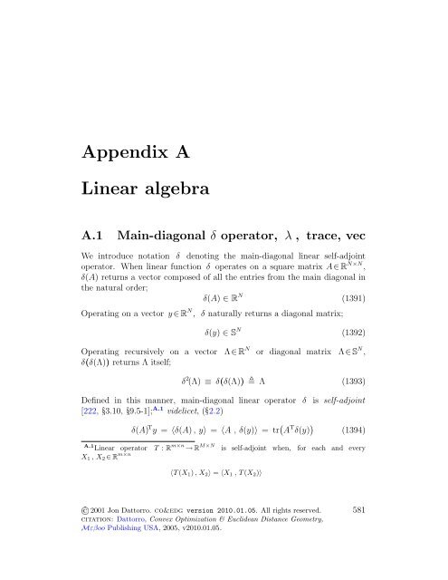
An important geometrical interpretation of SVD is given in Figure 152
for m = n = 2 : The image of the unit sphere under any m × n matrix
multiplication is an ellipse. Considering the three factors of the SVD
separately, note that Q T is a pure rotation of the circle. Figure 152 shows
how the axes q 1 and q 2 are first rotated by Q T to coincide with the coordinate
axes. Second, the circle is stretched by Σ in the directions of the coordinate
axes to form an ellipse. The third step rotates the ellipse by U into its
final position. Note how q 1 and q 2 are rotated to end up as u 1 and u 2 , the
principal axes of the final ellipse. A direct calculation shows that Aq j = σ j u j .
Thus q j is first rotated to coincide with the j th coordinate axis, stretched by
a factor σ j , and then rotated to point in the direction of u j . All of this
is beautifully illustrated for 2 ×2 matrices by the Matlab code eigshow.m
(see [328]).
A direct consequence of the geometric interpretation is that the largest
singular value σ 1 measures the “magnitude” of A (its 2-norm):
‖A‖ 2 = sup ‖Ax‖ 2 = σ 1 (1540)
‖x‖ 2 =1
This means that ‖A‖ 2 is the length of the longest principal semiaxis of the
ellipse.

A.6. SINGULAR VALUE DECOMPOSITION, SVD 613
Σ
q 2
q
q 2
1
Q T
q 1
q 2 u 2
U
u 1
q 1
Figure 152: Geometrical interpretation of full SVD [265]: Image of circle
{x∈ R 2 | ‖x‖ 2 =1} under matrix multiplication Ax is, in general, an ellipse.
For the example illustrated, U [u 1 u 2 ]∈ R 2×2 , Q[q 1 q 2 ]∈ R 2×2 .

614 APPENDIX A. LINEAR ALGEBRA
Expressions for U , Q , and Σ follow readily from (1539),
AA T U = UΣΣ T and A T AQ = QΣ T Σ (1541)
demonstrating that the columns of U are the eigenvectors of AA T and the
columns of Q are the eigenvectors of A T A. −Muller, Magaia, & Herbst [265]
A.6.4
Pseudoinverse by SVD
Matrix pseudoinverse (E) is nearly synonymous with singular value
decomposition because of the elegant expression, given A = UΣQ T ∈ R m×n
A † = QΣ †T U T ∈ R n×m (1542)
that applies to all three flavors of SVD, where Σ † simply inverts nonzero
entries of matrix Σ .
Given symmetric matrix A∈ S n and its diagonalization A = SΛS T
(A.5.1), its pseudoinverse simply inverts all nonzero eigenvalues:
A † = SΛ † S T ∈ S n (1543)
A.6.5
SVD of symmetric matrices
From (1532) and (1528) for A = A T
⎧√ (√
⎨ λ(A2 ) i = λ A 2)
= |λ(A) i | > 0, 1 ≤ i ≤ ρ
σ(A) i =
i
⎩
0, ρ < i ≤ η
(1544)
A.6.5.0.1 Definition. Step function. (confer4.3.2.0.1)
Define the signum-like quasilinear function ψ : R n → R n that takes value 1
corresponding to a 0-valued entry in its argument:
[
ψ(a)
lim
x i →a i
x i
|x i | = { 1, ai ≥ 0
−1, a i < 0 , i=1... n ]
∈ R n (1545)
△

A.7. ZEROS 615
Eigenvalue signs of a symmetric matrix having diagonalization
A = SΛS T (1525) can be absorbed either into real U or real Q from the
full SVD; [343, p.34] (conferC.4.2.1)
or
A = SΛS T = Sδ(ψ(δ(Λ))) |Λ|S T U ΣQ T ∈ S n (1546)
A = SΛS T = S|Λ|δ(ψ(δ(Λ)))S T UΣ Q T ∈ S n (1547)
where matrix of singular values Σ = |Λ| denotes entrywise absolute value of
diagonal eigenvalue matrix Λ .
A.7 Zeros
A.7.1
norm zero
For any given norm, by definition,
‖x‖ l
= 0 ⇔ x = 0 (1548)
Consequently, a generally nonconvex constraint in x like ‖Ax − b‖ = κ
becomes convex when κ = 0.
A.7.2
0 entry
If a positive semidefinite matrix A = [A ij ] ∈ R n×n has a 0 entry A ii on its
main diagonal, then A ij + A ji = 0 ∀j . [266,1.3.1]
Any symmetric positive semidefinite matrix having a 0 entry on its main
diagonal must be 0 along the entire row and column to which that 0 entry
belongs. [155,4.2.8] [198,7.1, prob.2]
A.7.3 0 eigenvalues theorem
This theorem is simple, powerful, and widely applicable:
A.7.3.0.1 Theorem. Number of 0 eigenvalues.
For any matrix A∈ R m×n
rank(A) + dim N(A) = n (1549)

616 APPENDIX A. LINEAR ALGEBRA
by conservation of dimension. [198,0.4.4]
For any square matrix A∈ R m×m , the number of 0 eigenvalues is at least
equal to dim N(A)
dim N(A) ≤ number of 0 eigenvalues ≤ m (1550)
while the eigenvectors corresponding to those 0 eigenvalues belong to N(A).
[325,5.1] A.17
For diagonalizable matrix A (A.5), the number of 0 eigenvalues is
precisely dim N(A) while the corresponding eigenvectors span N(A). The
real and imaginary parts of the eigenvectors remaining span R(A).
(TRANSPOSE.)
Likewise, for any matrix A∈ R m×n
rank(A T ) + dim N(A T ) = m (1551)
For any square A∈ R m×m , the number of 0 eigenvalues is at least equal
to dim N(A T ) = dim N(A) while the left-eigenvectors (eigenvectors of A T )
corresponding to those 0 eigenvalues belong to N(A T ).
For diagonalizable A , the number of 0 eigenvalues is precisely
dim N(A T ) while the corresponding left-eigenvectors span N(A T ). The real
and imaginary parts of the left-eigenvectors remaining span R(A T ). ⋄
Proof. First we show, for a diagonalizable matrix, the number of 0
eigenvalues is precisely the dimension of its nullspace while the eigenvectors
corresponding to those 0 eigenvalues span the nullspace:
Any diagonalizable matrix A∈ R m×m must possess a complete set of
linearly independent eigenvectors. If A is full-rank (invertible), then all
m=rank(A) eigenvalues are nonzero. [325,5.1]
A.17 We take as given the well-known fact that the number of 0 eigenvalues cannot be less
than dimension of the nullspace. We offer an example of the converse:
⎡ ⎤
1 0 1 0
A = ⎢ 0 0 1 0
⎥
⎣ 0 0 0 0 ⎦
1 0 0 0
dim N(A) = 2, λ(A) = [0 0 0 1] T ; three eigenvectors in the nullspace but only two are
independent. The right-hand side of (1550) is tight for nonzero matrices; e.g., (B.1) dyad
uv T ∈ R m×m has m 0-eigenvalues when u ∈ v ⊥ .

A.7. ZEROS 617
Suppose rank(A)< m . Then dim N(A) = m−rank(A). Thus there is
a set of m−rank(A) linearly independent vectors spanning N(A). Each
of those can be an eigenvector associated with a 0 eigenvalue because
A is diagonalizable ⇔ ∃ m linearly independent eigenvectors. [325,5.2]
Eigenvectors of a real matrix corresponding to 0 eigenvalues must be real. A.18
Thus A has at least m−rank(A) eigenvalues equal to 0.
Now suppose A has more than m−rank(A) eigenvalues equal to 0.
Then there are more than m−rank(A) linearly independent eigenvectors
associated with 0 eigenvalues, and each of those eigenvectors must be in
N(A). Thus there are more than m−rank(A) linearly independent vectors
in N(A) ; a contradiction.
Diagonalizable A therefore has rank(A) nonzero eigenvalues and exactly
m−rank(A) eigenvalues equal to 0 whose corresponding eigenvectors
span N(A).
By similar argument, the left-eigenvectors corresponding to 0 eigenvalues
span N(A T ).
Next we show when A is diagonalizable, the real and imaginary parts of
its eigenvectors (corresponding to nonzero eigenvalues) span R(A) :
The (right-)eigenvectors of a diagonalizable matrix A∈ R m×m are linearly
independent if and only if the left-eigenvectors are. So, matrix A has
a representation in terms of its right- and left-eigenvectors; from the
diagonalization (1513), assuming 0 eigenvalues are ordered last,
A =
m∑
λ i s i wi T =
i=1
k∑
≤ m
i=1
λ i ≠0
λ i s i w T i (1552)
From the linearly independent dyads theorem (B.1.1.0.2), the dyads {s i w T i }
must be independent because each set of eigenvectors are; hence rankA = k ,
the number of nonzero eigenvalues. Complex eigenvectors and eigenvalues
are common for real matrices, and must come in complex conjugate pairs for
the summation to remain real. Assume that conjugate pairs of eigenvalues
appear in sequence. Given any particular conjugate pair from (1552), we get
the partial summation
λ i s i w T i + λ ∗ i s ∗ iw ∗T
i = 2re(λ i s i w T i )
= 2 ( res i re(λ i w T i ) − im s i im(λ i w T i ) ) (1553)
A.18 Proof. Let ∗ denote complex conjugation. Suppose A=A ∗ and As i =0. Then
s i = s ∗ i ⇒ As i =As ∗ i ⇒ As ∗ i =0. Conversely, As∗ i =0 ⇒ As i=As ∗ i ⇒ s i= s ∗ i .

618 APPENDIX A. LINEAR ALGEBRA
where A.19 λ ∗ i λ i+1 , s ∗ i s i+1 , and w ∗ i w i+1 . Then (1552) is
equivalently written
A = 2 ∑ i
λ ∈ C
λ i ≠0
res 2i re(λ 2i w T 2i) − im s 2i im(λ 2i w T 2i) + ∑ j
λ ∈ R
λ j ≠0
λ j s j w T j (1554)
The summation (1554) shows: A is a linear combination of real and imaginary
parts of its (right-)eigenvectors corresponding to nonzero eigenvalues. The
k vectors {re s i ∈ R m , ims i ∈ R m | λ i ≠0, i∈{1... m}} must therefore span
the range of diagonalizable matrix A .
The argument is similar regarding the span of the left-eigenvectors.
A.7.4
0 trace and matrix product
For X,A∈ R M×N
+ (39)
tr(X T A) = 0 ⇔ X ◦ A = A ◦ X = 0 (1555)
For X,A∈ S M +
[33,2.6.1, exer.2.8] [352,3.1]
tr(XA) = 0 ⇔ XA = AX = 0 (1556)
Proof. (⇐) Suppose XA = AX = 0. Then tr(XA)=0 is obvious.
(⇒) Suppose tr(XA)=0. tr(XA)= tr( √ AX √ A) whose argument is
positive semidefinite by Corollary A.3.1.0.5. Trace of any square matrix is
equivalent to the sum of its eigenvalues. Eigenvalues of a positive semidefinite
matrix can total 0 if and only if each and every nonnegative eigenvalue is 0.
The only positive semidefinite matrix, having all 0 eigenvalues, resides at the
origin; (confer (1580)) id est,
√
AX
√
A =
(√
X
√
A
) T√
X
√
A = 0 (1557)
implying √ X √ A = 0 which in turn implies √ X( √ X √ A) √ A = XA = 0.
Arguing similarly yields AX = 0.
Diagonalizable matrices A and X are simultaneously diagonalizable if and
only if they are commutative under multiplication; [198,1.3.12] id est, iff
they share a complete set of eigenvectors.
A.19 Complex conjugate of w is denoted w ∗ . Conjugate transpose is denoted w H = w ∗T .

A.7. ZEROS 619
A.7.4.0.1 Example. An equivalence in nonisomorphic spaces.
Identity (1556) leads to an unusual equivalence relating convex geometry to
traditional linear algebra: The convex sets, given A ≽ 0
{X | 〈X , A〉 = 0} ∩ {X ≽ 0} ≡ {X | N(X) ⊇ R(A)} ∩ {X ≽ 0} (1558)
(one expressed in terms of a hyperplane, the other in terms of nullspace and
range) are equivalent only when symmetric matrix A is positive semidefinite.
We might apply this equivalence to the geometric center subspace, for
example,
S M c = {Y ∈ S M | Y 1 = 0}
= {Y ∈ S M | N(Y ) ⊇ 1} = {Y ∈ S M | R(Y ) ⊆ N(1 T )}
(1957)
from which we derive (confer (970))
S M c ∩ S M + ≡ {X ≽ 0 | 〈X , 11 T 〉 = 0} (1559)
A.7.5
Zero definite
The domain over which an arbitrary real matrix A is zero definite can exceed
its left and right nullspaces. For any positive semidefinite matrix A∈ R M×M
(for A +A T ≽ 0)
{x | x T Ax = 0} = N(A +A T ) (1560)
because ∃R A+A T =R T R , ‖Rx‖=0 ⇔ Rx=0, and N(A+A T )= N(R).
Then given any particular vector x p , x T pAx p = 0 ⇔ x p ∈ N(A +A T ). For
any positive definite matrix A (for A +A T ≻ 0)
Further, [386,3.2, prob.5]
{x | x T Ax = 0} = 0 (1561)
{x | x T Ax = 0} = R M ⇔ A T = −A (1562)
while
{x | x H Ax = 0} = C M ⇔ A = 0 (1563)

620 APPENDIX A. LINEAR ALGEBRA
The positive semidefinite matrix
[ ] 1 2
A =
0 1
for example, has no nullspace. Yet
(1564)
{x | x T Ax = 0} = {x | 1 T x = 0} ⊂ R 2 (1565)
which is the nullspace of the symmetrized matrix. Symmetric matrices are
not spared from the excess; videlicet,
[ ] 1 2
B =
(1566)
2 1
has eigenvalues {−1, 3} , no nullspace, but is zero definite on A.20
X {x∈ R 2 | x 2 = (−2 ± √ 3)x 1 } (1567)
A.7.5.0.1 Proposition. (Sturm/Zhang) Dyad-decompositions. [331,5.2]
Let positive semidefinite matrix X ∈ S M + have rank ρ . Then given symmetric
matrix A∈ S M , 〈A, X〉 = 0 if and only if there exists a dyad-decomposition
ρ∑
X = x j xj T (1568)
satisfying
j=1
〈A , x j x T j 〉 = 0 for each and every j ∈ {1... ρ} (1569)
⋄
The dyad-decomposition of X proposed is generally not that obtained
from a standard diagonalization by eigenvalue decomposition, unless ρ =1
or the given matrix A is simultaneously diagonalizable (A.7.4) with X .
That means, elemental dyads in decomposition (1568) constitute a generally
nonorthogonal set. Sturm & Zhang give a simple procedure for constructing
the dyad-decomposition [Wıκımization]; matrix A may be regarded as a
parameter.
A.20 These two lines represent the limit in the union of two generally distinct hyperbolae;
id est, for matrix B and set X as defined
lim
ε→0 +{x∈ R2 | x T Bx = ε} = X

A.7. ZEROS 621
A.7.5.0.2 Example. Dyad.
The dyad uv T ∈ R M×M (B.1) is zero definite on all x for which either
x T u=0 or x T v=0;
{x | x T uv T x = 0} = {x | x T u=0} ∪ {x | v T x=0} (1570)
id est, on u ⊥ ∪ v ⊥ . Symmetrizing the dyad does not change the outcome:
{x | x T (uv T + vu T )x/2 = 0} = {x | x T u=0} ∪ {x | v T x=0} (1571)