v2001.06.18 - Convex Optimization

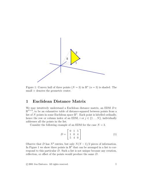
2
5
1
Figure 1: Convex hull of three points (N = 3) in R n (n = 3) is shaded. The
small × denotes the geometric center.
1 Euclidean Distance Matrix
We may intuitively understand a Euclidean distance matrix, an EDM D ∈
R N×N , to be an exhaustive table of distance-squared between points from a
list of N points in some Euclidean space R n . Each point is labelled ordinally,
hence the row or column index of an EDM, i or j ∈ {1...N}, individually
addresses all the points in the list.
Consider the following example of an EDM for the case N = 3.
⎡
D = ⎣
0 1 5
1 0 4
5 4 0
⎤
⎦ (1)
Observe that D has N 2 entries, but only N(N − 1)/2 pieces of information.
In Figure 1 we show three points in R 3 that can be arranged in a list to correspond
to this particular D. Such a list is not unique because any rotation,
reflection, or offset of the points would produce the same D.
c○ 2001 Jon Dattorro. All rights reserved. 1

1.1 Metric space requirements
If by d ij we denote the i,j th entry of the EDM D, then the distances-squared
{d ij , i,j = 1...N} must satisfy the requirements imposed by any metric
space:
1. √ d ij ≥ 0, i ≠ j (positivity)
2. d ij = 0, i = j (self-distance)
3. d ij = d ji (symmetry)
4. √ d ik + √ d kj ≥ √ d ij (triangle inequality)
where √ d ij is the Euclidean distance metric in R n . Hence an EDM must
be symmetric D = D T and its main diagonal zero, δ(D) = 0. If we assume
the points in R n are distinct, then entries off the main diagonal must be
strictly positive { √ d ij > 0, i ≠ j}. The last three metric space requirements
together imply nonnegativity of the { √ d ij }, not strict positivity, [6] but
prohibit D from having otherwise arbitrary symmetric entries off the main
diagonal. To enforce strict positivity we introduce another matrix criterion.
1.1.1 Strict positivity
The strict positivity criterion comes about when we require each x l to be
distinct; meaning, no entries of D except those along the main diagonal
δ(D) are zero. We claim that strict positivity {d ij > 0, i ≠ j} is controlled
by the strict matrix inequality −V T N DV N ≻ 0, symmetry D T = D, and the
self-distance criterion δ(D) = 0. 1
To support our claim, we introduce a full-rank skinny matrix V N having
the attribute R(V N ) = N(1 T );
⎡
⎤
−1 −1 · · · −1
V N = √ 1
1 0
1
∈ R N×N−1 (2)
N ⎢
⎥
⎣
... ⎦
0 1
1 Nonnegativity is controlled by relaxing the strict inequality.
2

If any square matrix A is positive definite, then its main diagonal δ(A) must
have all strictly positive elements. [4] For any D = D T and δ(D) = 0, it
follows that
− VNDV T N ≻ 0 ⇒ δ(−VNDV T N ) = ⎢
⎣
⎡
⎤
d 12
d 13
⎥
.
d 1N
⎦ ≻ 0 (3)
Multiplication of V N by any permutation matrix Ξ has null effect on its
range. In other words, any permutation of the rows or columns of V N produces
a basis for N(1 T ); id est, R(ΞV N ) = R(V N Ξ) = R(V N ) = N(1 T ).
Hence, the matrix inequality −VN TDV N ≻ 0 implies −VN TΞT DΞV N ≻ 0 (and
−Ξ T VN TDV NΞ ≻ 0). Various permutation matrices will sift the remaining d ij
similarly to (3) thereby proving their strict positivity. 2
♦
1.2 EDM definition
Ascribe the points in a list {x l ∈ R n , l = 1...N} to the columns of a matrix
X;
X = [x 1 · · · x N ] ∈ R n×N (4)
The entries of D are related to the points constituting the list like so:
d ij = ‖x i − x j ‖ 2 = ‖x i ‖ 2 + ‖x j ‖ 2 − 2x T i x j (5)
For D to be EDM it must be expressible in terms of some X,
D(X) = δ(X T X)1 T + 1δ T (X T X) − 2X T X (6)
where δ(A) means the column vector formed from the main diagonal of the
matrix A. When we say D is EDM, reading directly from (6), it implicitly
means D = D T and δ(D) = 0 are matrix criteria (but we already knew that).
If each x l is distinct, then {d ij > 0, i ≠ j}; in matrix terms, −V T N DV N ≻ 0.
Otherwise, −V T N DV N ≽ 0 when each x l is not distinct.
2 The rule of thumb is: if Ξ(i,1) = 1, then δ(−V T N ΞT DΞV N ) is some permutation of
the nonzero elements from the i th row or column of D.
3

1.3 Embedding Dimension
The convex hull of any list (or set) of points in Euclidean space forms a closed
(or solid) polyhedron whose vertices are the points constituting the list; [2]
conv{x l , l = 1...N} = {Xa | a T 1 = 1, a ≽ 0} (7)
The boundary and relative interior of that polyhedron constitute the convex
hull. The convex hull is the smallest convex set that contains the list. For the
particular example in Figure 1, the convex hull is the closed triangle while
its three vertices constitute the list.
The lower bound on Euclidean dimension consistent with an EDM D is
called the embedding (or affine) dimension, r. The embedding dimension r
is the dimension of the smallest hyperplane in R n that contains the convex
hull of the list in X. Dimension r is the same as the dimension of the convex
hull of the list X contains, but r is not necessarily equal to the rank of
X. 3 The fact r ≤ min {n,N − 1} can be visualized from the example in
Figure 1. There we imagine a vector from the origin to each point in the
list. Those three vectors are linearly independent in R 3 , but the embedding
dimension r equals 2 because the three points lie in a plane (the unique plane
in which the points are embedded; the plane that contains their convex hull),
the embedding plane (or affine hull). In other words, the three points are
linearly independent with respect to R 3 , but dependent with respect to the
embedding plane.
Embedding dimension is important because we lose any offset component
common to all the x l in R n when determining position given only distance
information. To calculate the embedding dimension, we first eliminate any
offset that serves to increase the dimensionality of the subspace required to
contain the convex hull; subtracting any point in the embedding plane from
every list member will work. We choose the geometric center 4 of the {x l };
c g = 1 N X1 ∈ Rn (8)
Subtracting the geometric center from all the points like so, X −c g 1 T , translates
their geometric center to the origin in R n . The embedding dimension
3 rank(X) ≤ min {n,N}
4 If we were to associate a point-mass m l with each of the points x l in a list, then their
center of mass (or gravity) would be c = ( ∑ x l m l )/ ∑ m l . The geometric center is the
same as the center of mass under the assumption of uniform mass density across points. [5]
The geometric center always lies in the convex hull.
4

is then r = rank(X − c g 1 T ). In general, we say that the {x l ∈ R n } and their
convex hull are embedded in some hyperplane, the embedding hyperplane
whose dimension is r. It is equally accurate to say that the {x l − c g } and
their convex hull are embedded in some subspace of R n whose dimension is
r.
It will become convenient to define a matrix V that arises naturally as
a consequence of translating the geometric center to the origin. Instead of
X − c g 1 T we may write XV ; viz.,
X − c g 1 T = X − 1 N X11T = X(I − 1 N 11T ) = XV ∈ R n×N (9)
Obviously,
V = V T = I − 1 N 11T ∈ R N×N (10)
so we may write the embedding dimension r more simply;
r = dim conv{x l , l = 1...N}
= rank(X − c g 1 T )
= rank(XV )
(11)
where V is an elementary matrix and a projection matrix. 5
r ≤ min {n,N − 1}
⇔
r ≤ n and r < N
(12)
5 A matrix of the form E = I − αuv T where α is a scalar and u and v are vectors
of the same dimension, is called an elementary matrix, or a rank-one modification of the
identity. [3] Any elementary matrix in R N×N has N − 1 eigenvalues equal to 1. For the
particular elementary matrix V , the remaining eigenvalue equals 0. Because V = V T
is diagonalizable, the number of zero eigenvalues must be equal to dim N(V T ) = 1, and
because V T 1 = 0, then N(V T ) = R(1). Because V = V T and V 2 = V , the elementary
matrix V is a projection matrix onto its range R(V ) = N(1 T ) having dimension N − 1.
5

1.4 Rotation, Reflection, Offset
When D is EDM, there exist an infinite number of corresponding N-point
lists in Euclidean space. All those lists are related by rotation, reflection,
and offset (translation).
If there were a common offset among all the x l , it would be cancelled in
the formation of each d ij . Knowing that offset in advance, call it c ∈ R n , we
might remove it from X by subtracting c1 T . Then by definition (6) of an
EDM, it stands to reason for any fixed offset c,
When c = c g we get
D(X − c1 T ) = D(X) (13)
D(X − c g 1 T ) = D(XV ) = D(X) (14)
In words, inter-point distances are unaffected by offset.
Rotation about some arbitrary point or reflection through some hyperplane
can be easily accomplished using an orthogonal matrix, call it Q. [9]
Again, inter-point distances are unaffected by rotation and reflection. We
rightfully expect that
D(QX − c1 T ) = D(Q(X − c1 T )) = D(QXV ) = D(QX) = D(XV ) (15)
So in the formation of the EDM D, any rotation, reflection, or offset
information is lost and there is no hope of recovering it. Reconstruction of
point position X can be guaranteed correct, therefore, only in the embedding
dimension r; id est, in relative position.
Because D(X) is insensitive to offset, we may safely ignore it and consider
only the impact of matrices that pre-multiply X; as in D(Q o X). The class
of pre-multiplying matrices for which inter-point distances are unaffected is
somewhat more broad than orthogonal matrices. Looking at definition (6),
it appears that any matrix Q o such that
X T Q T oQ o X = X T X (16)
will have the property D(Q o X) = D(X). That class includes skinny Q o having
orthonormal columns. Fat Q o are conceivable as long as (16) is satisfied.
6

2 EDM criteria
Given some arbitrary candidate matrix D, fundamental questions are: What
are the criteria for the entries of D sufficient to belong to an EDM, and what
is the minimum dimension r of the Euclidean space implied by EDM D?
2.1 Geometric condition
We continue considering the criteria necessary for a candidate matrix to be
EDM. We provide an intuitive geometric condition based upon the fact that
the convex hull of any list (or set) of points in Euclidean space R n is a closed
polyhedron.
We assert that D ∈ R N×N is a Euclidean distance matrix if and only if
distances-squared from the origin
{‖p‖ 2 = − 1 2 aT V T DV a | a T 1 = 1, a ≽ 0} (17)
are consistent with a point p ∈ R n in some closed polyhedron that is embedded
in a subspace of R n and has zero geometric center. (V as in (10).)
It is straightforward to show that the assertion is true in the forward
direction. We assume that D is indeed an EDM; id est, D comes from a list
of N unknown vertices in Euclidean space R n ; D = D(X) as in (6). Now
shift the geometric center of those unknown vertices to the origin, as in (9),
and then take any point p in their convex hull, as in (7);
{p = (X − c g 1 T )a = XV a | a T 1 = 1, a ≽ 0} (18)
Then any distance to the polyhedral convex hull can be formulated as
{p T p = ‖p‖ 2 = a T V T X T XV a | a T 1 = 1, a ≽ 0} (19)
Rearranging (6), X T X may be expressed
X T X = 1 2 (δ(XT X)1 T + 1δ T (X T X) − D) (20)
Substituting (20) into (19) yields (17) because V T 1 = 0.
To validate the assertion in the reverse direction, we must demonstrate
that if all distances-squared from the origin described by (17) are consistent
with a point p in some embedded polyhedron, then D is EDM. To show that,
7

2
1.5
1
0.5
y 2
0
−0.5
−1
−1.5
−2
−2 −1.5 −1 −0.5 0 0.5 1 1.5 2
y 1
Figure 2: Illustrated is a portion of the semi-infinite closed slab V y ≽ − 1 N 1
for N = 2 showing the inscribed ball of radius
1 √
N!
.
we must first derive an expression equivalent to (17). The condition a T 1 = 1
is equivalent to a = 1 N 1 + V y, where y ∈ RN , because R(V ) = N(1 T ).
Substituting a into (17),
{‖p‖ 2 = − 1 2 yT V T DV y | V y ≽ − 1 N 1, −V T DV ≽ 0} (21)
because V 2 = V . Because the solutions to V y ≽ − 1 1 constitute a semiinfinite
closed slab about the origin in R N (Figure 2), a ball of radius 1/ √ N!
N
centered at the origin can be fit into the interior. [10] Obviously it follows that
−V T DV must be positive semidefinite (PSD). 6 We may assume − 1V T DV is
2
symmetric 7 hence diagonalizable as QΛQ T ∈ R N×N . So, equivalent to (17) is
{‖p‖ 2 = a T QΛQ T a | a T 1 = 1, a ≽ 0, Λ ≽ 0} (22)
consistent with an embedded polyhedron by assumption. It remains to show
that D is EDM. Corresponding points {p = Λ 1/2 Q T a | a T 1 = 1, a ≽ 0, Λ ≽ 0}
∈ R N (n = N) 8 describe a polyhedron as in (7). Identify vertices XV =
6 ‖p‖ 2 ≥ 0 in all directions y, but that is not a sufficient condition for ‖p‖ 2 to be
consistent with a polyhedron.
7 The antisymmetric part (− 1 2 V T DV −(− 1 2 V T DV ) T )/2 of − 1 2 V T DV is benign in ‖p‖ 2 .
8 From (12) r < N, so we may always choose n equal to N when X is unknown.
8

Λ 1/2 Q T ∈ R N×N (X not unique, Section 1.4). Then D is EDM because it can
be expressed in the form of (6) by using the vertices we found. Applying (14),
D = D(X) = D(XV ) = D(Λ 1/2 Q T ) (23)
♦
9

2.2 Matrix criteria
In Section 2.1 we showed
D EDM
⇔
{‖p‖ 2 = − 1 2 aT V T DV a | a T 1 = 1, a ≽ 0} (17)
is consistent with some embedded polyhedron
⇒
−V T DV ≽ 0
(24)
while in Section 1.1.1 we learned that a strict matrix inequality −V T N DV N ≻ 0
{d ij > 0, i ≠ j}, −V T DV ≽ 0
⇐
D = D T , δ(D) = 0, −V T N DV N ≻ 0
(25)
yields distinction. Here we establish the necessary and sufficient conditions
for candidate D to be EDM; namely,
D EDM
⇔
D = D T , δ(D) = 0, −V T N DV N ≻ 0
(26)
We then consider the minimum dimension r of the Euclidean space implied
by EDM D.
10

Given D = D T , δ(D) = 0, and −V T DV ≻ 0, then by (24) and (25) it is
sufficient to show that (17) is consistent with some closed polyhedron that is
embedded in an r-dimensional subspace of R n and has zero geometric center.
Since − 1V T DV is assumed symmetric, it is diagonalizable as QΛQ T where
2
Q ∈ R N×N ,
[ ]
Λr 0
Λ = ∈ R N×N (27)
0 0
and where Λ r holds r strictly positive eigenvalues. As implied by (10), 1 ∈
N(− 1 2 V T DV ) ⇒ r < N like in (12), 9 so Λ must always have at least one 0
eigenvalue. Since − 1 2 V T DV is also assumed PSD, it is factorable;
− 1 2 V T DV = QΛ 1/2 Q T oQ o Λ 1/2 Q T (28)
where Q o ∈ R n×N is unknown as is its dimension n. Q o is constrained,
however, such that its first r columns are orthonormal. Its remaining columns
are arbitrary. We may then rewrite (17):
{p T p = a T QΛ 1/2 Q T oQ o Λ 1/2 Q T a | a T 1=1, a≽0, Λ 1/2 Q T oQ o Λ 1/2 = Λ ≽ 0} (29)
Then {p = Q o Λ 1/2 Q T a | a T 1 = 1, a ≽ 0, Λ 1/2 Q T oQ o Λ 1/2 = Λ ≽ 0} ∈ R n
describes a polyhedron as in (7) having vertices
XV = Q o Λ 1/2 Q T ∈ R n×N (30)
1
whose geometric center Q N oΛ 1/2 Q T 1 is the origin. 10 If we like, we may
choose n to be rank(Q o Λ 1/2 Q T ) = rank(Λ) = r which is the smallest n
possible. 11
♦
9 For any square matrix A, the number of 0 eigenvalues is at least equal to dim N(A).
For any diagonalizable matrix A, the number of 0 eigenvalues is exactly equal to dim N(A).
10 For any A, N(A T A) = N(A). [9] In our case,
N(− 1 2 V T DV ) = N(QΛQ T ) = N(QΛ 1/2 Q T o Q o Λ 1/2 Q T ) = N(Q o Λ 1/2 Q T ) = N(XV ).
⎡
⎤
⎥
⎦ in terms of eigen-
q T1 λ 1 0
11 If we write Q T = ⎣
. .. ⎦ ⎢ . ..
in terms of row vectors, Λ= ⎣ λr
qN
T 0 0
values, and Q o =[q o1 · · · q oN ] in terms of column vectors, then Q o Λ 1/2 Q T ∑
= r
⎡
⎤
is a sum of r linearly independent rank-one matrices. Hence the result has rank r.
11
i=1
λ 1/2
i q oi qi
T

Recall from (12), r < N and r ≤ n. n is finite but otherwise unbounded
above. Given an EDM D, then for any valid choice of n, there is an X ∈ R n×N
and a Q o ∈ R n×N having the property Λ 1/2 Q T oQ o Λ 1/2 = Λ, such that
D = D(X) = D(XV ) = D(Q o Λ 1/2 Q T ) = D(Λ 1/2 Q T ) (31)
2.2.1 Metric space requirements vs. matrix criteria
In Section 1.1.1 we demonstrated that the strict matrix inequality −V T N DV N ≻ 0
replaces the strict positivity criterion {d ij > 0, i ≠ j}. Comparing the three
criteria in (26) to the three requirements imposed by any metric space, enumerated
in Section 1.1, it appears that the strict matrix inequality is simultaneously
the matrix analog to the triangle inequality. Because the criteria
for the existence of an EDM must be identical to the requirements imposed
by a Euclidean metric space, we may conclude that the three criteria in (26)
are equivalent to the metric space requirements. So we have the analogous
criteria for an EDM:
1. −V T N DV N ≽ 0 (positivity)
2. δ(D) = 0 (self-distance)
3. D T = D (symmetry)
4. −V T N DV N ≽ 0 (triangle inequality)
If we replace the inequality with its strict version, then duplicate x l are not
allowed.
12

2.3 Cone of EDM
13

3 Map of the USA
Beyond fundamental questions regarding the characteristics of an EDM, a
more intriguing question is whether or not it is possible to reconstruct relative
point position given only an EDM.
The validation of our assertion is constructive. The embedding dimension
r may be determined by counting the number of nonzero eigenvalues.
Certainly from (11) we know that dim R(XV ) = r, which means some rows
of X found by way of (??) can always be truncated.
We may want to test our results thus far.
14

4 Spectral Analysis
The discrete Fourier transform (DFT) is a staple of the digital signal processing
community. [7] In essence, the DFT is a correlation of a windowed sequence
(or discrete signal) with exponentials whose frequencies are equally
spaced on the unit circle. 12 The DFT of the sequence {f(i) ∈ R,i = 0...n − 1}
is, in traditional form, 13 ∑n−1
F(k) = f(i)e −ji2πk/n (32)
i=0
for k = 0...n − 1 and j = √ −1. The implicit window on f(i) in (32) is
rectangular. The values {F(k) ∈ C, k = 0...n−1} are considered a spectral
analysis of the sequence f(i); id est, the F(k) are amplitudes of exponentials
which when combined, give back the original sequence,
f(i) = 1 ∑n−1
F(k)e ji2πk/n (33)
n
k=0
The argument of F, the index k, corresponds to the discrete frequencies
2πk/n of the exponentials e ji2πk/n in the synthesis equation (33).
The DFT (32) is separable in the real and the imaginary part; meaning,
the analysis exhibits no dependency between the two parts when the sequence
is real; viz.,
∑n−1
∑n−1
F(k) = f(i) cos(i2πk/n) − j f(i) sin(i2πk/n) (34)
i=0
It follows then, to relate the DFT to our work with EDMs, we should separately
consider the Euclidean distance-squared between the sequence and
each part of the complex exponentials. Augmenting the real list of polyhedral
vertices {x l ∈ R n , l = 1...N} will be the new imaginary list {y l ∈ R n ,
l = 1...N}, where
i=0
x 1 = [f(i), i = 0...n − 1]
y 1 = [f(i), i = 0...n − 1]
x l = [ cos(i2π(l − 2)/n), i = 0...n − 1],
y l = [− sin(i2π(l − 2)/n), i = 0...n − 1],
l = 2...N
l = 2...N
(35)
12 the unit circle in the z plane; z = e sT where s = σ + jω is the traditional Laplace
frequency, ω is the Fourier frequency in radians 2πf, while T is the sample period.
13 The convention is lowercase for the sequence and uppercase for its transform.
15

where N = n + 1, and where the [ ] bracket notation means a vector made
from a sequence. The row-1 elements (columns l = 2...N) of EDM D x are
d x 1l = n−1 ∑
(x l − x 1 ) 2
i=0
= n−1 ∑
i=0
= n−1 ∑
= 1 4
i=0
(cos(i2π(l − 2)/n) − f(i)) 2
cos 2 (i2π(l − 2)/n) + f 2 (i) − 2f(i) cos(i2π(l − 2)/n)
sin(2π(l(2n−1)+2)/n)
(2n + 1 + ) + 1 sin(2π(l−2)/n) n
n−1 ∑
k=0
|F(k)| 2 − 2 RF(l − 2)
(36)
where R takes the real part of its argument, and where the Fourier summation
is from the Parseval relation for the DFT. 14 [7] For the imaginary vertices
we have a separate EDM D y whose row-1 elements (columns l = 2...N) are
d y 1l = n−1 ∑
(y l − y 1 ) 2
i=0
= n−1 ∑
i=0
= n−1 ∑
= 1 4
i=0
(sin(i2π(l − 2)/n) + f(i)) 2
sin 2 (i2π(l − 2)/n) + f 2 (i) + 2f(i) sin(i2π(l − 2)/n)
sin(2π(l(2n−1)+2)/n)
(2n − 1 − ) + 1 sin(2π(l−2)/n) n
n−1 ∑
k=0
|F(k)| 2 − 2 IF(l − 2)
(37)
where I takes the imaginary part of its argument. In the remaining rows
(m = 2...N, m < l) of these two EDMs, D x and D y , we have 15
d x ml = n−1 ∑
(cos(i2π(l − 2)/n) − cos(i2π(m − 2)/n)) 2
i=0
= 1 sin(2π(l(2n−1)+2)/n)
(4n + 2 +
4 sin(2π(l−2)/n)
d y ml = n−1 ∑
= 1 4
i=0
+ sin(2π(m(2n−1)+2)/n)
sin(2π(m−2)/n)
)
(sin(i2π(l − 2)/n) − sin(i2π(m − 2)/n)) 2
(4n − 2 −
sin(2π(l(2n−1)+2)/n)
sin(2π(l−2)/n)
− sin(2π(m(2n−1)+2)/n)
sin(2π(m−2)/n)
)
(38)
14 The Fourier summation ∑ |F(k)| 2 /n replaces ∑ f 2 (i); we arbitrarily chose not to mix
domains. Some physical systems, such as Magnetic Resonance Imaging devices, naturally
produce signals originating in the Fourier domain. [11]
15 sin(2π(i(2n−1)+2)/n)
lim
i→2
sin(2π(i−2)/n)
= 2n − 1
16

We observe from these distance-squared equations that only the first row and
column of the EDM depends upon the sequence itself. The remainder of the
EDM depends only upon the sequence length n.
17

To relate the EDMs D x and D y to the DFT in a useful way, we consider
finding the inverse DFT (IDFT) via either EDM. For reasonable values of
N, the number of matrix entries N 2 can become prohibitively large. But the
DFT is subject to the same order of computational intensity. The matrix
form of the DFT is written
F = Wf (39)
where F = [F(k), k = 0...n − 1], f = [f(i), i = 0...n − 1], and the DFT
matrix is [8]
⎡
⎤
1 1 1 · · · 1
1 e −j2πk/n e −j4πk/n · · · e −j(n−1)2πk/n
W = W T 1 e −j4πk/n e −j8πk/n · · · e −j(n−1)4πk/n
=
1 e −j6πk/n e −j12πk/n · · · e −j(n−1)6πk/n
(40)
⎢
⎥
⎣ . . . · · · . ⎦
1 e −j(n−1)2πk/n e −j(n−1)4πk/n · · · e −j(n−1)2 2πk/n
When presented in this non-traditional way, the size of the DFT matrix
W ∈ R n×n becomes apparent. It is obvious that a direct implementation of
(39) would require on the order of n 2 operations for large n. Similarly, the
IDFT is
f = 1 n WH F (41)
where we have taken the conjugate transpose of the DFT matrix.
The solution to the computational problem of evaluating the DFT for
large n culminated in the development of the fast Fourier transform (FFT)
algorithm whose intensity is proportional to n log(n). [7] It is neither our
purpose nor goal to invent a fast algorithm for doing this, we simply present
an example of finding the IDFT by way of the EDM. The technique we use
was developed in Section 2.1:
1. Diagonalize − 1 2 V T DV as QΛQ T ∈ R N×N .
2. Identify polyhedral vertices XV = Q o Λ 1/2 Q T ∈ R n×N where Q o is an
unknown rotation/reflection matrix, and where Λ ≽ 0 for an EDM.
18

5 Matrix completion problem
Even more intriguing is whether the positional information can be reconstructed
given an incomplete EDM.
19

A
loose ends
r = rank(XV ) = rank(V T X T XV ) = rank(−V T DV )
−V T DV ≽ 0 ⇔ −z T Dz ≥ 0 on z ∈ N(1 T )
tr(− 1 2 V T DV ) = 1 N
∑
i,j
d ij = 1
2N 1T D1
D(X) = D(XV ).
Then substitution of V T X T XV = − 1 2 V T DV ⇒
D = δ(− 1 2 V T DV )1 T + 1δ T (− 1 2 V T DV ) + V T DV
A.1 V w
⎡
V w =
⎢
⎣
−1 √
N
1 + −1
N+ √ N
−1
N+ √ N
.
−1
N+ √ N
√−1
−1
N
· · · √
N
−1
N+ √ N
· · ·
−1
N+ √ N
1 + −1
N+ √ · · · −1
N N+ √ N
.
... .
−1
N+ √ N
· · · 1 + −1
N+ √ N
⎤
∈ R N×N−1 (42)
⎥
⎦
V can be expressed in terms of the full rank matrix V w ; [1]
V = V w V T w (43)
where V T w V w = I. Hence the positive semidefinite criterion can be expressed
instead as −V T wDV w ≽ 0. 16
Equivalently, we may simply interpret V in the positive definite criterion
to mean any matrix whose range spans N(1 T ). The fact that V can be expressed
as in (43) shows that V is a projection matrix; all projection matrices
P can be expressed in the form P = QQ T where Q is an orthogonal matrix.
16 This is easily shown because V T w V w = I and −z T V T DV z ≥ 0 must be true for all z
including z = V w y.
20

References
[1] Abdo Y. Alfakih, Amir Khandani, and Henry Wolkowicz. Solving
Euclidean distance matrix completion problems via semidefinite programming.
Computational Optimization and Applications, 12(1):13–30,
January 1999.
http://citeseer.ist.psu.edu/alfakih97solving.html
[2] Stephen Boyd and Lieven Vandenberghe. Convex Optimization.
http://www.stanford.edu/~boyd/cvxbook
[3] Philip E. Gill, Walter Murray, and Margaret H. Wright. Practical Optimization.
Academic Press, 1999.
[4] Gene H. Golub and Charles F. Van Loan. Matrix Computations. Johns
Hopkins, third edition, 1996.
[5] George B. Thomas, Jr. Calculus and Analytic Geometry.
Addison-Wesley, fourth edition, 1972.
[6] Erwin Kreyszig. Introductory Functional Analysis with Applications.
Wiley, 1989.
[7] Alan V. Oppenheim and Ronald W. Schafer. Discrete-Time Signal
Processing. Prentice-Hall, 1989.
[8] Boaz Porat. A Course in Digital Signal Processing. Wiley, 1997.
[9] Gilbert Strang. Linear Algebra and its Applications. Harcourt Brace,
third edition, 1988.
[10] William Wooton, Edwin F. Beckenbach, and Frank J. Fleming. Modern
Analytic Geometry. Houghton Mifflin, 1975.
[11] Graham A. Wright. An introduction to magnetic resonance.
www.sunnybrook.utoronto.ca:8080/~gawright/main mr.html .
21