sparse image representation via combined transforms - Convex ...

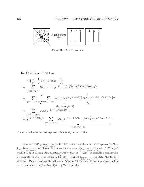
156 APPENDIX B. FAST EDGELET-LIKE TRANSFORM
1 2 3
4 X-interpolate
5 =⇒
6
1 2 3 4 5 6
Figure B.1: X-interpolation.
For 0 ≤ k, l ≤ N − 1, we have
=
=
=
( k
F
N − 1 2 2)
,s(k)+l · ∆(k) − 1
∑
i=0,1,... ,N−1;
j=0,1,... ,N−1.
∑
j=0,1,... ,N−1
∑
j=0,1,... ,N−1
I(i +1,j+1)e −2π√ −1( k N − 1 2 )i e −2π√ −1(s(k)+l·∆(k)− 1 2 )j
⎛
⎝
= e −2π√ −1∆(k) l2 2 ·
∑
i=0,1,... ,N−1
⎞
I(i +1,j+1)e −2π√ −1( k N − 1 2 )i ⎠
} {{ }
define as g(k, j)
g(k, j)e −2π√ −1(s(k)+l·∆(k)− 1 2 )j
∑
j=0,1,... ,N−1
e −2π√ −1(s(k)+l·∆(k)− 1 2 )j
g(k, j)e −2π√ −1(j·s(k)− 1 2 j+∆(k) j2 2 ) · e π√ −1∆(k)(l−j) 2
.
} {{ }
convolution.
The summation in the last expression is actually a convolution.
The matrix (g(k, j)) k=0,1,... ,N−1 is the 1-D Fourier transform of the image matrix I(i +
j=0,1,... ,N−1
1,j+1) i=0,1,... ,N−1 by column. We can compute matrix (g(k, j)) k=0,1,... ,N−1 with O(N 2 log N)
j=0,1,... ,N−1
j=0,1,... ,N−1
work. For fixed k, computing function value F ( k N
,s(k)+l · ∆(k)) is basically a convolution.
To compute the kth row in matrix ( F ( k N ,s(k)+l · ∆(k))) k=0,1,... ,N−1 , we utilize the Toeplitz
l=0,1,... ,N−1
structure. We can compute the kth row in O(N log N) time, and hence computing the first
half of the matrix in (B.4) has O(N 2 log N) complexity.