sparse image representation via combined transforms - Convex ...
sparse image representation via combined transforms - Convex ... sparse image representation via combined transforms - Convex ...
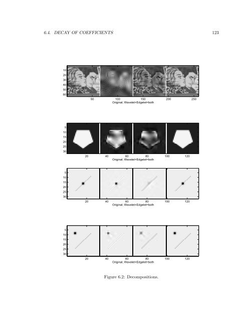
122 CHAPTER 6. SIMULATIONS fourth sub-image should be close to the original. We have some interesting observations: 1. Overall, we observe the wavelet parts possess features resembling points (fine scale wavelets) and patches (coarse scale scaling functions), while the edgelet parts possess features resembling lines. This is most obvious in Car and least obvious in Pentagon. The reason could be that Pentagon does not contain many linear features. (Boundaries are not lines.) 2. We observe some artifacts in the decompositions. For example, in the wavelet part of Car, we see a lot of fine scale features that are not similar to points, but are similar to line segments. This implies that they are made by many small wavelets. The reason for this is the intrinsic disadvantage of the edgelet-like transform that we have used. As in Figure B.3, the representers of our edgelet-like transform have a fixed width. This prevents it from efficiently representing narrow features. The same phenomena emerge in Overlap and Separate. A way to overcome it is to develop a transform whose representers have not only various locations, lengths and orientations, but also various widths. This will be an interesting topic of future research. 6.4 Decay of Coefficients As we discussed in Chapter 2, one can measure sparsity of representation by studying the decay of the coefficient amplitudes. The faster the decay of coefficient amplitudes, the sparser the representation. We compare our approach with two other approaches. One is an approach using merely the 2-D DCT; the other is an approach using merely the discrete 2-D wavelet transform. The reasons we choose to compare with these transforms: 1. The 2-D DCT, especially the one localized to 8 × 8 blocks, has been applied in an important industry standard for image compression and transmission known as JPEG. 2. The 2-D wavelet transform is a modern alternative to 2-D DCT. In some developing industry standards (e.g., draft standards for JPEG-2000), the 2-D wavelet transform has been adopted as an option. It has been proven to be more efficient than 2-D DCT in many cases.
6.4. DECAY OF COEFFICIENTS 123 10 20 30 40 50 60 50 100 150 200 250 Original; Wavelet+Edgelet=both 5 10 15 20 25 30 20 40 60 80 100 120 Original; Wavelet+Edgelet=both 5 10 15 20 25 30 20 40 60 80 100 120 Original; Wavelet+Edgelet=both 5 10 15 20 25 30 20 40 60 80 100 120 Original; Wavelet+Edgelet=both Figure 6.2: Decompositions.
- Page 99 and 100: 3.4. OTHER TRANSFORMS 71 Folding. A
- Page 101 and 102: 3.4. OTHER TRANSFORMS 73 We can app
- Page 103 and 104: 3.5. DISCUSSION 75 give only a few
- Page 105 and 106: 3.7. PROOFS 77 the ijth component o
- Page 107 and 108: 3.7. PROOFS 79 Similarly, we have [
- Page 109 and 110: Chapter 4 Combined Image Representa
- Page 111 and 112: 4.2. SPARSE DECOMPOSITION 83 interi
- Page 113 and 114: 4.3. MINIMUM l 1 NORM SOLUTION 85 l
- Page 115 and 116: 4.4. LAGRANGE MULTIPLIERS 87 ρ( x
- Page 117 and 118: 4.5. HOW TO CHOOSE ρ AND λ 89 3 (
- Page 119 and 120: 4.6. HOMOTOPY 91 A way to interpret
- Page 121 and 122: 4.7. NEWTON DIRECTION 93 4.7 Newton
- Page 123 and 124: 4.9. ITERATIVE METHODS 95 1. Avoidi
- Page 125 and 126: 4.11. DISCUSSION 97 ρ(β) =‖β
- Page 127 and 128: 4.12. PROOFS 99 4.12.2 Proof of The
- Page 129 and 130: 4.12. PROOFS 101 case of (4.16). Co
- Page 131 and 132: Chapter 5 Iterative Methods This ch
- Page 133 and 134: 5.1. OVERVIEW 105 the k-th iteratio
- Page 135 and 136: 5.1. OVERVIEW 107 5.1.4 Preconditio
- Page 137 and 138: 5.2. LSQR 109 among all the block d
- Page 139 and 140: 5.2. LSQR 111 5.2.3 Algorithm LSQR
- Page 141 and 142: 5.3. MINRES 113 2. For k =1, 2,...,
- Page 143 and 144: 5.3. MINRES 115 using the precondit
- Page 145 and 146: 5.4. DISCUSSION 117 From (I + S 1 )
- Page 147 and 148: Chapter 6 Simulations Section 6.1 d
- Page 149: 6.3. DECOMPOSITION 121 10 5 5 5 20
- Page 153 and 154: 6.5. COMPARISON WITH MATCHING PURSU
- Page 155 and 156: 6.6. SUMMARY OF COMPUTATIONAL EXPER
- Page 157 and 158: Chapter 7 Future Work In the future
- Page 159 and 160: 7.2. MODIFYING EDGELET DICTIONARY 1
- Page 161 and 162: 7.3. ACCELERATING THE ITERATIVE ALG
- Page 163 and 164: Appendix A Direct Edgelet Transform
- Page 165 and 166: A.2. EXAMPLES 137 edgelet transform
- Page 167 and 168: A.3. DETAILS 139 (a) Stick image (b
- Page 169 and 170: A.3. DETAILS 141 (a) Lenna image (b
- Page 171 and 172: A.3. DETAILS 143 Ordering of Dyadic
- Page 173 and 174: A.3. DETAILS 145 (1,K +1), (1,K +2)
- Page 175 and 176: A.3. DETAILS 147 x 1 , y 1 x 2 , y
- Page 177 and 178: Appendix B Fast Edgelet-like Transf
- Page 179 and 180: B.1. TRANSFORMS FOR 2-D CONTINUOUS
- Page 181 and 182: B.2. DISCRETE ALGORITHM 153 B.2.1 S
- Page 183 and 184: B.2. DISCRETE ALGORITHM 155 extensi
- Page 185 and 186: B.2. DISCRETE ALGORITHM 157 For the
- Page 187 and 188: B.3. ADJOINT OF THE FAST TRANSFORM
- Page 189 and 190: B.4. ANALYSIS 161 above matrix, whi
- Page 191 and 192: B.5. EXAMPLES 163 B.5 Examples B.5.
- Page 193 and 194: B.5. EXAMPLES 165 And so on. Note f
- Page 195 and 196: B.6. MISCELLANEOUS 167 It takes abo
- Page 197 and 198: B.6. MISCELLANEOUS 169 The function
- Page 199 and 200: Bibliography [1] Sensor Data Manage
6.4. DECAY OF COEFFICIENTS 123<br />
10<br />
20<br />
30<br />
40<br />
50<br />
60<br />
50 100 150 200 250<br />
Original; Wavelet+Edgelet=both<br />
5<br />
10<br />
15<br />
20<br />
25<br />
30<br />
20 40 60 80 100 120<br />
Original; Wavelet+Edgelet=both<br />
5<br />
10<br />
15<br />
20<br />
25<br />
30<br />
20 40 60 80 100 120<br />
Original; Wavelet+Edgelet=both<br />
5<br />
10<br />
15<br />
20<br />
25<br />
30<br />
20 40 60 80 100 120<br />
Original; Wavelet+Edgelet=both<br />
Figure 6.2: Decompositions.


