Economic Models - Convex Optimization

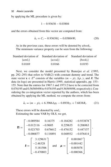
32 Alexis Lazaridis
by applying the ML procedure is given by:
1 − 0.93638 − 0.03804
and the errors obtained from this vector are computed from:
û i = C i − 0.93638I i − 0.03804W i (20)
As in the previous case, these errors will be denoted by ubook i .
The minimum variance property can be seen from the following:
Standard deviation of Standard deviation of Standard deviation of
{uml i } {usvd i } {book i }
0.0169 0.0166 0.0193
Next, we consider the model presented by Banerjee et al. (1993,
pp. 292–293) that refers to VAR(2) with constant dummy and trend. The
state vector x ∈ E 4 consists of the variables (m − p), p, y, and R. The
data (in logs) are presented in Harris (1995, statistical appendix, pp. 153–
155. Note that the entries for 1967:1 and 1973:2 have to be corrected from
0.076195 and 0.56569498 to 9.076195 and 9.56569498, respectively). Considering
the co-integration vector reported by the authors, which has been
obtained by applying the ML method, we compute the errors from:
û i = (m − p) i + 6.3966p i − 0.8938y i + 7.6838R i . (21)
These errors will be denoted by uml i .
Estimating the same VAR by OLS, we get,
⎡
⎤
−0.089584 0.16375 −0.184282 −0.933878
−0.012116 −0.9605 0.229635 0.206963
= ⎢
⎥
⎣ 0.021703 0.676612 −0.476152 0.447157 ⎦ ,
−0.006877 0.118891 0.048932 −0.076414
⎡ ⎤
⎡ ⎤
3.129631
0.001867
−2.46328
δ = ⎢ ⎥
⎣ 5.181506 ⎦ and µ =
−0.001442
⎢ ⎥
⎣ 0.003078 ⎦
−0.470803
−0.000366