Assignment 5: EOSC 352
Assignment 5: EOSC 352
Assignment 5: EOSC 352

Create successful ePaper yourself
Turn your PDF publications into a flip-book with our unique Google optimized e-Paper software.
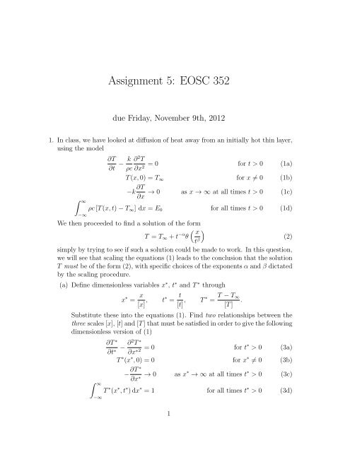
<strong>Assignment</strong> 5: <strong>EOSC</strong> <strong>352</strong><br />
due Friday, November 9th, 2012<br />
1. In class, we have looked at diffusion of heat away from an initially hot thin layer,<br />
using the model<br />
∫ ∞<br />
−∞<br />
∂T<br />
∂t − k ∂ 2 T<br />
= 0<br />
ρc ∂x2 for t > 0 (1a)<br />
T (x, 0) = T ∞ for x ≠ 0 (1b)<br />
−k ∂T → 0<br />
∂x<br />
as x → ∞ at all times t > 0 (1c)<br />
ρc [T (x, t) − T ∞ ] dx = E 0 for all times t > 0 (1d)<br />
We then proceeded to find a solution of the form<br />
( x<br />
)<br />
T = T ∞ + t −α θ<br />
t β<br />
simply by trying to see if such a solution could be made to work. In this question,<br />
we will see that scaling the equations (1) leads to the conclusion that the solution<br />
T must be of the form (2), with specific choices of the exponents α and β dictated<br />
by the scaling procedure.<br />
(a) Define dimensionless variables x ∗ , t ∗ and T ∗ through<br />
x ∗ = x<br />
[x] ,<br />
t∗ = t<br />
[t] ,<br />
T ∗ = T − T ∞<br />
.<br />
[T ]<br />
Substitute these into the equations (1). Find two relationships between the<br />
three scales [x], [t] and [T ] that must be satisfied in order to give the following<br />
dimensionless version of (1)<br />
∫ ∞<br />
−∞<br />
∂T ∗<br />
∂t ∗<br />
− ∂2 T ∗<br />
∂x ∗2 = 0 for t∗ > 0 (3a)<br />
T ∗ (x ∗ , 0) = 0 for x ∗ ≠ 0 (3b)<br />
− ∂T ∗<br />
∂x → 0 ∗ as x∗ → ∞ at all times t ∗ > 0 (3c)<br />
T ∗ (x ∗ , t ∗ ) dx ∗ = 1 for all times t ∗ > 0 (3d)<br />
1<br />
(2)
Is it possible to define [x], [t] and [T ] uniquely in terms of the model parameters<br />
E 0 , k, ρ and c?<br />
(b) Let γ be a positive number, and let<br />
t ∗∗ = γt ∗ , x ∗∗ = γ β x ∗ , T ∗∗ = γ −α T ∗<br />
where α and β are exponents to be determined. Substitute the new variables<br />
into (3). Show that one can find α and β such that, for any γ > 0, the system<br />
of equations (3) is transformed into<br />
∫ ∞<br />
−∞<br />
∂T ∗∗<br />
∂t − ∂2 T ∗∗<br />
∗∗ ∂x = 0 for ∗2 t∗∗ > 0 (4a)<br />
T ∗∗ (x ∗∗ , 0) = 0 for x ∗∗ ≠ 0 (4b)<br />
∂T<br />
∗∗<br />
−<br />
∂x → 0 as ∗∗ x∗∗ → ∞ at all times t ∗∗ > 0 (4c)<br />
T ∗∗ (x ∗∗ , t ∗∗ ) dx ∗∗ = 1 for all times t ∗∗ > 0 (4d)<br />
Give the relevant values of α and β.<br />
(c) It is clear that (4) is the same as (3) except that T ∗ has been replaced by T ∗∗ ,<br />
x ∗ by x ∗∗ and t ∗ by t ∗∗ . This is known as a scale invariance of the equations<br />
(3). In essence, we see that the equations stay the same if we stretch our<br />
length, time and temperature scales in a particular way. What this means is<br />
that the physics of the problem actually looks ‘the same’ at different scales,<br />
and hence the solution will also look ‘the same’. We will show that this<br />
implies a self-similar solution of the form (2). If the set of equations (3)<br />
has a unique solution, then it is clear that the dependent variable T ∗∗ must<br />
therefore depend on the independent variables x ∗∗ and t ∗∗ in the same way<br />
as the dependent variable T ∗ depends on the independent variables x ∗ and<br />
t ∗ . In other words, if T ∗ can be written as a function of x ∗ and t ∗ in the<br />
form<br />
T ∗ = f(x ∗ , t ∗ )<br />
then<br />
T ∗∗ = f(x ∗∗ , t ∗∗ )<br />
with the same function f in both equations. Use the definition of T ∗∗ , x ∗∗<br />
and t ∗∗ to show that this means that<br />
f(x ∗ , t ∗ ) = γ α f(γ β x ∗ , γt ∗ ).<br />
But γ is arbitrary, so for any given t ∗ , we can choose γ = t ∗−1 . Show that it<br />
therefore follows that<br />
( ) x<br />
T ∗ = t ∗−α ∗<br />
f<br />
t , 1 .<br />
∗β<br />
Choosing ξ ∗ = x ∗ /t ∗β , θ ∗ (ξ ∗ ) = f(ξ ∗ , 1) then leads to the similarity solution<br />
form (2).<br />
Page 2
2. In class, we derived the similarity solution<br />
to the problem (1).<br />
T (x, t) = t −1/2 C exp<br />
(<br />
− ρc<br />
4k<br />
)<br />
x 2<br />
+ T ∞<br />
t<br />
(a) Sketch the form of T (x, t) as a function of x for some fixed time t > 0.<br />
(b) Compute heat flux as a function of x for fixed t > 0. Sketch the form of heat<br />
flux as a function of x on the same graph as above.<br />
(c) Compute the divergence of heat flux as a function of x for fixed t > 0.<br />
Sketch this on the same graph as above. Where is temperature increasing,<br />
and where is it decreasing?<br />
(d) Next, take a fixed position x > 0, and (on a separate graph) sketch how<br />
T (x, t) evolves over time at that fixed position x.<br />
(e) For any fixed x > 0, temperature reaches a maximum. Compute the time at<br />
which this maximum occurs as a function of x (as well as ρ, c and k), and<br />
compute the maximum temperature reached in terms of x, ρ, c, k and C.<br />
(f) To get a full solution, we still need to relate C to E 0 . We have<br />
∫ ∞<br />
−∞<br />
ρc [T (x, t) − T ∞ ] dx = E 0 .<br />
To use this to compute C in terms of E 0 , we need to be able to compute<br />
∫ ∞<br />
−∞<br />
exp ( −x 2) dx.<br />
There is a trick to doing this: consider<br />
[∫ ∞<br />
exp ( −x 2) 2 [∫ ∞<br />
dx]<br />
= exp ( −x 2) ] [∫ ∞<br />
dx × exp ( −y 2) ]<br />
dy<br />
−∞<br />
−∞<br />
−∞<br />
=<br />
∫ ∞ ∫ ∞<br />
−∞<br />
−∞<br />
exp ( −(x 2 + y 2) dx dy<br />
But, if we define r 2 = x 2 + y 2 , this is simply the integral of exp(−r 2 ) over<br />
the entire xy-plane, which can be done in polar coordinates:<br />
∫ ∞ ∫ ∞<br />
exp ( −(x 2 + y 2) ∫ 2π<br />
[∫ ∞<br />
]<br />
dx dy = exp(−r 2 )r dr dθ.<br />
−∞<br />
−∞<br />
By evaluating the integral in polar coordinates, show that<br />
∫ ∞<br />
−∞<br />
exp ( −x 2) dx = √ π<br />
0<br />
0<br />
Page 3
(g) Suppose that E 0 represents the excess heat (beyond the amount of heat<br />
associated with the background temperature T ∞ ) contained in a dyke of<br />
narrow width d filled with hot rock (of the same density ρ and heat capacity<br />
c as the surrounding rock) at an initial temperature T 0 , find C in terms of<br />
T 0 , T ∞ and d.<br />
(h) Suppose the dyke has a width of d = 2 cm, and the initial temperature of the<br />
rock in the dyke is T 0 = 2000 K. Suppose also that the rock surrounding the<br />
dyke has ρ = 2700 kg m −3 , c = 10 3 J kg −1 K −1 and k = 2 W m −1 K −1 , and<br />
that it has a background temperature of T ∞ = 600 K. You are told that the<br />
rock surrounding the dyke is chemically altered if raised to a temperature<br />
T > 1000 K. Once the heat in the dyke has been completely conducted away,<br />
how far do you have to be away from the rock to find chemically unaltered<br />
rock?<br />
Page 4