Mechanical APDL Basic Analysis Guide - Ansys
Mechanical APDL Basic Analysis Guide - Ansys Mechanical APDL Basic Analysis Guide - Ansys
Chapter 2: Loading Boundary Condition Bulk Temperature (Convection) Heat Flux Heat Generation Uniform Heat Generation Structural Analyses Displacements Hydrostatic Pressure Forces and Moments Fluid Mass Flow Rate Pressures Temperature Linear Acceleration Translational Acceleration Superelement Load Vector Magnetic Analyses Current Density Electrical Analyses Voltage Current Primary Variable TIME, X, Y, Z TIME, X, Y, Z, TEMP TIME, X, Y, Z, TEMP TIME TIME or FREQ, X, Y, Z, TEMP TIME or FREQ, X, Y, Z, TEMP TIME or FREQ, X, Y, Z, TEMP, SECTOR TIME or FREQ, X, Y, Z, TEMP, SECTOR TIME or FREQ, X, Y, Z, TEMP, SECTOR TIME, X, Y, Z, TEMP TIME or FREQ, X, Y, Z TIME or FREQ, X, Y, Z TIME TIME, X, Y, Z TIME, X, Y, Z TIME, X, Y, Z High-Frequency Electromagnetic Analyses Current Density Fluid Analyses Pressure Flow FLOTRAN Analyses Nodal DOF Nodal DOF for ALE formulation 50 TIME, X, Y, Z TIME, X, Y, Z TIME, X, Y, Z TIME, X, Y, Z, TEMP, VELO- CITY, PRESSURE TIME, X, Y, Z, TEMP, VELO- CITY, PRES, Xr, Yr, Zr Command [1] SFE,,,CONV SF,,,TBULK SFE,,,TBULK SF,,HFLUX SFE,,,HFLUX BFE,,HGEN BFUNIF,TEMP D,(UX, UY, UZ, ROTX, ROTY, ROTZ) D,HDSP F,(FX, FY, FZ, MX, MY, MZ) F,DVOL SF,,PRES SFE,,,PRES BF,,TEMP BFE,,TEMP ACEL,ACEL_X, ACEL_Y,ACEL_Z CMACEL,CMACEL_X, CMACEL_Y,CMACEL_Z SFE,,,SELV BFE,,JS D,,VOLT F,,AMPS BFE,,JS D,,PRES F,,FLOW D,,(VX, VY, VZ, PRES, TEMP, ENKE, ENDS, SP01-SP06) D,,(UX, UY, UZ) Release 13.0 - © SAS IP, Inc. All rights reserved. - Contains proprietary and confidential information of ANSYS, Inc. and its subsidiaries and affiliates.
Boundary Condition Heat Flux Film Coefficient Element Heat Generation Nodal Heat Generation Nodal Body Force Radiation Fluid Volume Primary Variable TIME, X, Y, Z, TEMP, VELO- CITY, PRESSURE TIME, X, Y, Z, TEMP, VELO- CITY, PRESSURE TIME, X, Y, Z, TEMP, VELO- CITY, PRESSURE TIME, X, Y, Z, TEMP, VELO- CITY, PRESSURE TIME, X, Y, Z, TEMP, VELO- CITY, PRESSURE TIME, X, Y, Z, TEMP, VELO- CITY, PRESSURE TIME, X, Y, Z, TEMP, VELO- CITY, PRESSURE Command [1] SF,,HFLUX SFE,,,HFLUX SF,,CONV SFE,,,CONV BFE,,HGEN BF,,HGEN BF,,FORCE SF,,RAD SFE,,,RAD SF,,VFRC SFE,,,VFRC 1. Although not normally used in this manner, the following commands also allow tabular loading: BFA, BFK, BFL, BFV, DA, DK, DL, FK, SFA, and SFL. See the *DIM command for more information on defining your labels. The VELOCITY label refers to the magnitude of the velocity degrees of freedom or the computed fluid velocity in FLUID116 elements. In addition, some real constants for elements SURF151, SURF152, and FLUID116 can have associated primary variables. Table 2.12 Real Constants and Corresponding Primary Variable Real Constants SURF151, SURF152 Rotational Speed FLUID116 Rotational Speed Slip Factor Primary Variables TIME, X, Y, Z TIME, X, Y, Z TIME, X, Y, Z 2.5.14.2. Defining Independent Variables 2.5.14. Applying Loads Using TABLE Type Array Parameters If you need to specify a variable other than one of the primary variables listed, you can do so by defining an independent parameter. To specify an independent parameter, you define an additional table for the independent parameter. That table must have the same name as the independent parameter, and can be a function of either a primary variable or another independent parameter. You can define as many independent parameters as necessary, but all independent parameters must relate to a primary variable. For example, consider a convection coefficient (HF) that varies as a function of rotational speed (RPM) and temperature (TEMP). The primary variable in this case is TEMP. The independent parameter is RPM, which Release 13.0 - © SAS IP, Inc. All rights reserved. - Contains proprietary and confidential information of ANSYS, Inc. and its subsidiaries and affiliates. 51
- Page 15 and 16: List of Tables 2.1. DOF Constraints
- Page 17 and 18: Chapter 1: Getting Started with ANS
- Page 19 and 20: shown below define two element type
- Page 21 and 22: You can choose constant, isotropic,
- Page 23 and 24: You can save linear material proper
- Page 25 and 26: Figure 1.4 Material Model Interface
- Page 27 and 28: Figure 1.7 Data Input Dialog Box -
- Page 29 and 30: The first example below is intended
- Page 31 and 32: 9. Click on OK. The dialog box clos
- Page 33 and 34: 1.1.4.9. Reading a Material Library
- Page 35 and 36: If you are performing a static or f
- Page 37 and 38: Chapter 2: Loading The primary obje
- Page 39 and 40: Figure 2.2 Transient Load History C
- Page 41 and 42: The arc-length method is an advance
- Page 43 and 44: • Transferred solid loads will re
- Page 45 and 46: Note If the node rotation angles th
- Page 47 and 48: Figure 2.7 Scaling Temperature Cons
- Page 49 and 50: Below are examples of some of the G
- Page 51 and 52: Utility Menu> List> Loads> Surface>
- Page 53 and 54: Figure 2.9 Example of Surface Load
- Page 55 and 56: the shell, and 270° to 360° for t
- Page 57 and 58: Below are examples of some of the G
- Page 59 and 60: Figure 2.15 Transfers to BFK Loads
- Page 61 and 62: CASE C: At least one BFV, BFA, or B
- Page 63 and 64: A handy way to specify density so t
- Page 65: For more information, see Initial S
- Page 69 and 70: This problem consists of a thermal-
- Page 71 and 72: 2.6. Specifying Load Step Options A
- Page 73 and 74: - All loads changed in later load s
- Page 75 and 76: Main Menu> Preprocessor> Loads> Loa
- Page 77 and 78: Command GUI Menu Paths Main Menu> S
- Page 79 and 80: ! Load Step 1: D, ... ! Loads SF, .
- Page 81 and 82: Modeling> Create> Elements> Auto Nu
- Page 83 and 84: Figure 2.22 Pretension Section Samp
- Page 85 and 86: cylind,0.35,1, 0.75,1, 0,180 wpstyl
- Page 87 and 88: 11. Select Utility Menu> PlotCtrls>
- Page 89 and 90: 24. Select Utility Menu> Plot> Comp
- Page 91 and 92: Chapter 3: Using the Function Tool
- Page 93 and 94: Hint: A common error is a divide-by
- Page 95 and 96: 3.3. Using the Function Loader When
- Page 97 and 98: 2. Define the convection boundary c
- Page 99 and 100: 7. Optional: Enter comments for thi
- Page 101 and 102: 3.6.1. Graphing a Function From the
- Page 103 and 104: Chapter 4: Initial State The term i
- Page 105 and 106: inis,defi,,,1,,100,200,150 inis,def
- Page 107 and 108: applies an equal stress of SX = 100
- Page 109 and 110: 4.7.2. Example: Initial Stress Prob
- Page 111 and 112: inis,defi,all,all,all,all,0.1,,, in
- Page 113 and 114: Chapter 5: Solution In the solution
- Page 115 and 116: Solver Typical Applications * In to
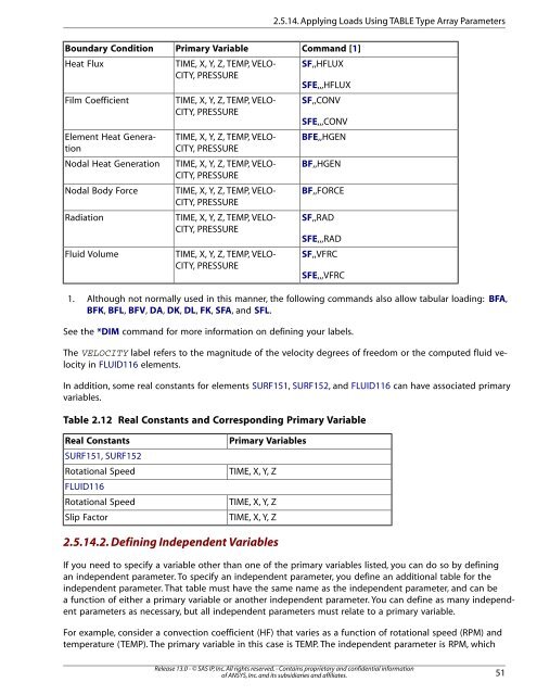
Boundary Condition<br />
Heat Flux<br />
Film Coefficient<br />
Element Heat Generation<br />
Nodal Heat Generation<br />
Nodal Body Force<br />
Radiation<br />
Fluid Volume<br />
Primary Variable<br />
TIME, X, Y, Z, TEMP, VELO-<br />
CITY, PRESSURE<br />
TIME, X, Y, Z, TEMP, VELO-<br />
CITY, PRESSURE<br />
TIME, X, Y, Z, TEMP, VELO-<br />
CITY, PRESSURE<br />
TIME, X, Y, Z, TEMP, VELO-<br />
CITY, PRESSURE<br />
TIME, X, Y, Z, TEMP, VELO-<br />
CITY, PRESSURE<br />
TIME, X, Y, Z, TEMP, VELO-<br />
CITY, PRESSURE<br />
TIME, X, Y, Z, TEMP, VELO-<br />
CITY, PRESSURE<br />
Command [1]<br />
SF,,HFLUX<br />
SFE,,,HFLUX<br />
SF,,CONV<br />
SFE,,,CONV<br />
BFE,,HGEN<br />
BF,,HGEN<br />
BF,,FORCE<br />
SF,,RAD<br />
SFE,,,RAD<br />
SF,,VFRC<br />
SFE,,,VFRC<br />
1. Although not normally used in this manner, the following commands also allow tabular loading: BFA,<br />
BFK, BFL, BFV, DA, DK, DL, FK, SFA, and SFL.<br />
See the *DIM command for more information on defining your labels.<br />
The VELOCITY label refers to the magnitude of the velocity degrees of freedom or the computed fluid velocity<br />
in FLUID116 elements.<br />
In addition, some real constants for elements SURF151, SURF152, and FLUID116 can have associated primary<br />
variables.<br />
Table 2.12 Real Constants and Corresponding Primary Variable<br />
Real Constants<br />
SURF151, SURF152<br />
Rotational Speed<br />
FLUID116<br />
Rotational Speed<br />
Slip Factor<br />
Primary Variables<br />
TIME, X, Y, Z<br />
TIME, X, Y, Z<br />
TIME, X, Y, Z<br />
2.5.14.2. Defining Independent Variables<br />
2.5.14. Applying Loads Using TABLE Type Array Parameters<br />
If you need to specify a variable other than one of the primary variables listed, you can do so by defining<br />
an independent parameter. To specify an independent parameter, you define an additional table for the<br />
independent parameter. That table must have the same name as the independent parameter, and can be<br />
a function of either a primary variable or another independent parameter. You can define as many independent<br />
parameters as necessary, but all independent parameters must relate to a primary variable.<br />
For example, consider a convection coefficient (HF) that varies as a function of rotational speed (RPM) and<br />
temperature (TEMP). The primary variable in this case is TEMP. The independent parameter is RPM, which<br />
Release 13.0 - © SAS IP, Inc. All rights reserved. - Contains proprietary and confidential information<br />
of ANSYS, Inc. and its subsidiaries and affiliates.<br />
51


