- Page 1 and 2: ANSYS Mechanical APDL Basic Analysi
- Page 3 and 4: Table of Contents 1. Getting Starte
- Page 5 and 6: 2.8.4.3. Define Material Properties
- Page 7 and 8: 7.2.1.6. Particle Flow and Charged
- Page 9 and 10: 10. Getting Started with Graphics .
- Page 11 and 12: 13.2.4.1.Turning Load Symbols and C
- Page 13 and 14: 20.8. Reviewing Contents of Binary
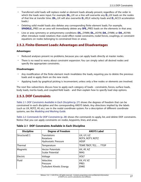
- Page 15 and 16: List of Tables 2.1. DOF Constraints
- Page 17 and 18: Chapter 1: Getting Started with ANS
- Page 19 and 20: shown below define two element type
- Page 21 and 22: You can choose constant, isotropic,
- Page 23 and 24: You can save linear material proper
- Page 25 and 26: Figure 1.4 Material Model Interface
- Page 27 and 28: Figure 1.7 Data Input Dialog Box -
- Page 29 and 30: The first example below is intended
- Page 31 and 32: 9. Click on OK. The dialog box clos
- Page 33 and 34: 1.1.4.9. Reading a Material Library
- Page 35 and 36: If you are performing a static or f
- Page 37 and 38: Chapter 2: Loading The primary obje
- Page 39 and 40: Figure 2.2 Transient Load History C
- Page 41: The arc-length method is an advance
- Page 45 and 46: Note If the node rotation angles th
- Page 47 and 48: Figure 2.7 Scaling Temperature Cons
- Page 49 and 50: Below are examples of some of the G
- Page 51 and 52: Utility Menu> List> Loads> Surface>
- Page 53 and 54: Figure 2.9 Example of Surface Load
- Page 55 and 56: the shell, and 270° to 360° for t
- Page 57 and 58: Below are examples of some of the G
- Page 59 and 60: Figure 2.15 Transfers to BFK Loads
- Page 61 and 62: CASE C: At least one BFV, BFA, or B
- Page 63 and 64: A handy way to specify density so t
- Page 65 and 66: For more information, see Initial S
- Page 67 and 68: Boundary Condition Heat Flux Film C
- Page 69 and 70: This problem consists of a thermal-
- Page 71 and 72: 2.6. Specifying Load Step Options A
- Page 73 and 74: - All loads changed in later load s
- Page 75 and 76: Main Menu> Preprocessor> Loads> Loa
- Page 77 and 78: Command GUI Menu Paths Main Menu> S
- Page 79 and 80: ! Load Step 1: D, ... ! Loads SF, .
- Page 81 and 82: Modeling> Create> Elements> Auto Nu
- Page 83 and 84: Figure 2.22 Pretension Section Samp
- Page 85 and 86: cylind,0.35,1, 0.75,1, 0,180 wpstyl
- Page 87 and 88: 11. Select Utility Menu> PlotCtrls>
- Page 89 and 90: 24. Select Utility Menu> Plot> Comp
- Page 91 and 92: Chapter 3: Using the Function Tool
- Page 93 and 94:
Hint: A common error is a divide-by
- Page 95 and 96:
3.3. Using the Function Loader When
- Page 97 and 98:
2. Define the convection boundary c
- Page 99 and 100:
7. Optional: Enter comments for thi
- Page 101 and 102:
3.6.1. Graphing a Function From the
- Page 103 and 104:
Chapter 4: Initial State The term i
- Page 105 and 106:
inis,defi,,,1,,100,200,150 inis,def
- Page 107 and 108:
applies an equal stress of SX = 100
- Page 109 and 110:
4.7.2. Example: Initial Stress Prob
- Page 111 and 112:
inis,defi,all,all,all,all,0.1,,, in
- Page 113 and 114:
Chapter 5: Solution In the solution
- Page 115 and 116:
Solver Typical Applications * In to
- Page 117 and 118:
used. Running the distributed spars
- Page 119 and 120:
With all iterative solvers, be part
- Page 121 and 122:
5.3.3. Disk Space (I/O) and Postpro
- Page 123 and 124:
If your analysis is either static o
- Page 125 and 126:
Note Whether you make changes to on
- Page 127 and 128:
Figure 5.2 PGR File Options From th
- Page 129 and 130:
GUI: Main Menu> Solution> Current L
- Page 131 and 132:
Figure 5.3 Examples of Time-Varying
- Page 133 and 134:
Requirements for Performing an Anal
- Page 135 and 136:
*dim,temtbl,table,4,1,,time ! Defin
- Page 137 and 138:
5.9.1.1.1. Multiframe Restart Limit
- Page 139 and 140:
prnsol finish 5.9.2. VT Accelerator
- Page 141 and 142:
5.12. Stopping Solution After Matri
- Page 143 and 144:
Chapter 6: An Overview of Postproce
- Page 145 and 146:
each element. Derived data are also
- Page 147 and 148:
Chapter 7: The General Postprocesso
- Page 149 and 150:
Although not required for postproce
- Page 151 and 152:
The ETABLE command documentation li
- Page 153 and 154:
• Path plots • Reaction force d
- Page 155 and 156:
The PLETAB command contours data st
- Page 157 and 158:
PLDISP,1 ! Deformed shape superimpo
- Page 159 and 160:
7.2.1.6. Particle Flow and Charged
- Page 161 and 162:
• Particle flow traces occasional
- Page 163 and 164:
The surfaces you create fall into t
- Page 165 and 166:
You can opt to archive all defined
- Page 167 and 168:
19 41.811 51.777 .00000E+00 -66.760
- Page 169 and 170:
Sample PRETAB and SSUM Output *****
- Page 171 and 172:
7.2.5. Mapping Results onto a Path
- Page 173 and 174:
Command(s): PDEF GUI: Main Menu> Ge
- Page 175 and 176:
To retrieve path information from a
- Page 177 and 178:
7.2.6. Estimating Solution Error On
- Page 179 and 180:
Write Results - You can use the dat
- Page 181 and 182:
NOTE: When you append data to your
- Page 183 and 184:
EMF - Windows Enhanced Metafile For
- Page 185 and 186:
Figure 7.20 The PGR File Options Di
- Page 187 and 188:
7.4.8. Comparing Nodal Solutions Fr
- Page 189 and 190:
the effect of the rigid body rotati
- Page 191 and 192:
The SADD command (Main Menu> Genera
- Page 193 and 194:
To view correct mid-surface results
- Page 195 and 196:
To get usable results combine the r
- Page 197 and 198:
7.4.4. Mapping Results onto a Diffe
- Page 199 and 200:
• EMF (Main Menu> General Postpro
- Page 201 and 202:
7.4.8.1. Matching the Nodes The Mec
- Page 203 and 204:
7.4.8. Comparing Nodal Solutions Fr
- Page 205 and 206:
Chapter 8: The Time-History Postpro
- Page 207 and 208:
enables the alternate selections sh
- Page 209 and 210:
1. Click on the Add Data button. Re
- Page 211 and 212:
APPEND Appends data to previously s
- Page 213 and 214:
!derivative of variable 2 with resp
- Page 215 and 216:
The above command assumes that you
- Page 217 and 218:
When plotting complex data such as
- Page 219 and 220:
Sample Output from EXTREM time-hist
- Page 221 and 222:
5. Select the variables to be opera
- Page 223 and 224:
RESP requires two previously define
- Page 225 and 226:
Chapter 9: Selecting and Components
- Page 227 and 228:
Note Crossover commands for selecti
- Page 229 and 230:
would put UX and UZ constraints on
- Page 231 and 232:
The Command Reference describes the
- Page 233 and 234:
Chapter 10: Getting Started with Gr
- Page 235 and 236:
Remote Network Access Hidden Line R
- Page 237 and 238:
10.4.1. Adjusting Input Focus To en
- Page 239 and 240:
• If the environment variable SB_
- Page 241 and 242:
10.5.5. Erasing the Current Display
- Page 243 and 244:
Chapter 11: General Graphics Specif
- Page 245 and 246:
11.3.1. Changing the Viewing Direct
- Page 247 and 248:
11.4. Controlling Miscellaneous Tex
- Page 249 and 250:
11.4.3. Controlling the Location of
- Page 251 and 252:
Chapter 12: PowerGraphics Two metho
- Page 253 and 254:
The subgrid approach affects both t
- Page 255 and 256:
Chapter 13: Creating Geometry Displ
- Page 257 and 258:
Figure 13.1 Element Plot of SOLID65
- Page 259 and 260:
13.2.1.12. Vector Versus Raster Mod
- Page 261 and 262:
Figure 13.2 Create Best Quality Ima
- Page 263 and 264:
13.2.3.2. Choosing a Format for the
- Page 265 and 266:
Chapter 14: Creating Geometric Resu
- Page 267 and 268:
Figure 14.2 A Typical ANSYS Results
- Page 269 and 270:
• Changing the contour interval.
- Page 271 and 272:
14.5. Isosurface Techniques Isosurf
- Page 273 and 274:
Chapter 15: Creating Graphs If you
- Page 275 and 276:
Establishing separate Y-axis scales
- Page 277 and 278:
15.2.3.5. Defining the TIME (or, Fo
- Page 279 and 280:
Chapter 16: Annotation A common ste
- Page 281 and 282:
16.3. 3-D Annotation 3-D text and g
- Page 283 and 284:
Chapter 17: Animation Animation is
- Page 285 and 286:
• ANMODE (Utility Menu> PlotCtrls
- Page 287 and 288:
Figure 17.2 The Animation Controlle
- Page 289 and 290:
Note If you are doing animation fro
- Page 291 and 292:
Chapter 18: External Graphics Besid
- Page 293 and 294:
18.1.4. Exporting Graphics in UNIX
- Page 295 and 296:
Note The commands discussed in this
- Page 297 and 298:
18.3.6. Editing the Neutral Graphic
- Page 299 and 300:
Chapter 19: The Report Generator Th
- Page 301 and 302:
2. Specify a caption for the captur
- Page 303 and 304:
19.4.1.1. Creating a Custom Table I
- Page 305 and 306:
Table ID 46 47 48 Description Compo
- Page 307 and 308:
Button or Field DYNAMIC DATA REPORT
- Page 309 and 310:
The HTML tag to begin JavaScript co
- Page 311 and 312:
listingName A unique listing name a
- Page 313 and 314:
Chapter 20: File Management and Fil
- Page 315 and 316:
20.4. Text Versus Binary Files Depe
- Page 317 and 318:
Identifier ELEM EMAT ERR ESAV FATG
- Page 319 and 320:
20.4.3. File Compression Many file
- Page 321 and 322:
You can also redirect graphics outp
- Page 323 and 324:
Chapter 21: Memory Management and C
- Page 325 and 326:
21.3.3. Changing Database Space Fro
- Page 327 and 328:
Figure 21.4 Dividing Work Space ANS
- Page 329 and 330:
NUM_BUFR is the number of buffers p
- Page 331 and 332:
een chosen for efficient running of
- Page 333 and 334:
Index Symbols 3-D graphics devices,
- Page 335 and 336:
path plots, 142 POST26 graphs, 200
- Page 337 and 338:
fatigue graphs, 257 files, 277 focu
- Page 339 and 340:
material model interface, 8 materia
- Page 341 and 342:
multiframe, 117 restarting an analy
- Page 343 and 344:
WINDOW command, 227 Windows graphic