Advanced Stochastic Processes.

More documents

Recommendations

Info

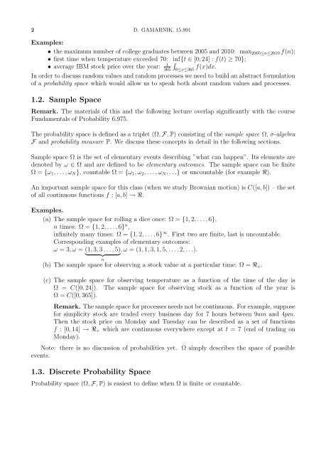
2 D. GAMARNIK, 15.991 Examples: • the maximum number of college graduates between 2005 and 2010: max 2005≤n≤2010 f(n); • first time when temperature exceeded 70: inf{t ∈ [0, 24] : f(t) ≥ 70}; • average IBM stock price over the year: 1 365 ∫ 0≤x≤365 f(x)dx. In order to discuss random values and random processes we need to build an abstract formulation of a probability space which would allow us to speak both about random values and processes. 1.2. Sample Space Remark. The materials of this and the following lecture overlap significantly with the course Fundamentals of Probability 6.975. The probability space is defined as a triplet (Ω, F, P) consisting of the sample space Ω, σ-algebra F and probability measure P. We discuss these concepts in detail in the following sections. Sample space Ω is the set of elementary events describing ”what can happen”. Its elements are denoted by ω ∈ Ω and are defined to be elementary outcomes. The sample space can be finite Ω = {ω 1 , . . . , ω N }, countable Ω = {ω 1 , ω 2 , . . . , ω N , . . .} or uncountable (for example R). An important sample space for this class (when we study Brownian motion) is C([a, b]) – the set of all continuous functions f : [a, b] → R. Examples. (a) The sample space for rolling a dice once: Ω = {1, 2, . . . , 6}, n times: Ω = {1, 2, . . . , 6} n , infinitely many times: Ω = {1, 2, . . . , 6} ∞ . First two are finite, last is uncountable. Corresponding examples of elementary outcomes: ω = 3, ω = (1, 3, 3 . . . , 5) , ω = (1, 1, 3, 1, 5, . . . , 2, . . .). } {{ } n (b) The sample space for observing a stock value at a particular time: Ω = R + . (c) The sample space for observing temperature as a function of the time of the day is Ω = C([0, 24]). The sample space for observing stock as a function of the year is Ω = C([0, 365]). Remark. The sample space for processes needs not be continuous. For example, suppose for simplicity stock are traded every business day for 7 hours between 9am and 4pm. Then the stock price on Monday and Tuesday can be described as a set of functions f : [0, 14] → R + which are continuous everywhere except at t = 7 (end of trading on Monday). Note: there is no discussion of probabilities yet. Ω simply describes the space of possible events. 1.3. Discrete Probability Space Probability space (Ω, F, P) is easiest to define when Ω is finite or countable.
LECTURE 1. PROBABILITY BASICS 3 Definition 1.1. A discrete probability space is a triplet (Ω, F, P) such that (a) The sample space Ω is finite or countable Ω = {ω 1 , ω 2 , . . .}; (b) F is the set of all subsets of Ω. (c) P is a function P : Ω → [0, 1] such that ∑ ω∈Ω P[ω] = 1. For every subset A ∈ F we define P[A] = ∑ ω∈A P[ω]. There is no need to describe F since it is the set of all subsets. Thus, we may simply write (Ω, P). Examples. (a) n unbiased coin tosses. Ω = {0, 1} n . P[ω] = 1/2 n . Suppose Then A = {ω = (ω 1 , . . . , ω n ) : ω 1 = 1, ω n = 0}. P[A] = ∑ ω:ω 1 =1,ω n=0 P[ω] = 2 n−2 1 2 n = 1 4 . (b) Geometric random variable. A parameter 0 < ρ < 1 is fixed. Ω = Z + . For every ω ∈ Ω, P[ω] = (1 − ρ)ρ ω . (c) Poisson random variable. A parameter λ > 0 is fixed. Ω = Z + . For every ω ∈ Ω, P[ω] = λ ω ω! e−λ . 1.4. σ-algebras When Ω is not countable it is not clear how to assign probabilities to elementary events. For example, we want to capture the intuition that a randomly chosen point from [0, 1] has a probability 1/4 of falling into [1/2, 3/4]. If we assign P[ω] to be a positive value c > 0 then we have a problem: the total sum ∑ ω P[w] = ∞. If we assign P[ω] = 0, how do we get P[1/2, 3/4] = 1/4? The solution is to assign probabilities to sets A ⊂ [0, 1] of elementary outcomes, instead of individual outcomes ω ∈ [0, 1]. For every A ⊂ Ω A c denotes the complement set: {ω ∈ Ω : ω /∈ A}. A collection of sets A 1 , A 2 , . . . ⊂ Ω is called mutually exclusive if A i ∩ A j = ∅ whenever i ≠ j. Definition 1.2. A σ-field F is a collection of subsets of Ω satisfying the following conditions: (a) Ω ∈ F (b) If A ∈ F then A c ∈ F. (c) If a sequence A 1 , A 2 , . . . ∈ F then ∪ i A i ∈ F. Any set A ∈ F is called measurable or F-measurable. σ-field replaces the set of all subsets A ⊂ Ω when Ω is no longer countable. Exercise 1. Given a σ-field F. Prove that if A, B ∈ F then A ∩ B ∈ F. In general, given an infinite sequence A 1 , A 2 , . . . , ∈ F prove that ∩ i A i ∈ F.
Page 1: Advanced Stochastic Processes. Davi
Page 5 and 6: LECTURE 1. PROBABILITY BASICS 5 Bor
Page 7 and 8: LECTURE 1. PROBABILITY BASICS 7 Def
Page 9: BIBLIOGRAPHY 1. R. Durrett, Probabi

Advanced Stochastic Processes.

Create successful ePaper yourself

Delete template?

Save as template?