0 - NMR Spectroscopy Research Group

Biomolecular High Resolution NMR in 

Utrecht 

WWW.NMR.CHEM.UU.NL 

Rainer Wechselberger, NMR Spectroscopy, Utrecht, 2009

Contact Informatie Docenten 

Hoorcollege: 

Werkcolleges: 

Rainer Wechselberger 

rwechsel@its.jnj.com 

Hans Wienk 

tel. 030 253 9928 

hans@nmr.chem.uu.nl 

Marloes Schurink 

tel. 030 253 9928 

m.schurink@uu.nl 

www.nmr.chem.uu.nl 


Rooster Hoorcollege NMR 

5 weken (07.10. t/m 02.11.) 

Locatie: Went Groen 

Tijden: Woensdag en Vrijdag 9:00 – 10:45 

www.chem.uu.nl: 

Onderwijs > Bachelor > Roosters2009-2010 > jaar2periode 1 


Tentamen S & A NMR 

GEEN OPEN BOEK!!! 

ma 2 november, 9 – 10.30 uur, Went Blauw 

Herkansing: vr 8 januari 2010, 14.00-15.30 K-128 


Het beste... 

... lees thuis voor het college de 

hoofdstukken van het dictaat... 

... lees thuis na het college de 

hoofdstukken van het dictaat... 

... maak eigen aantekeningen... 

... vraag direct alsietsnietduidelijkis! 


General Outline 

I Introduction (what is NMR and what is studied with it) 

II Basic Theory (how does it work) 

III Ensemble of spins (from single atom to real samples) 

IV Relaxation I (after the experiment: back to equilibrium) 

V FT NMR (with a single rf-pulse to a complete spectrum) 

VI Hardware (what kind of device do you need for NMR) 

VII NMR parameters (what you can see in an NMR spectrum) 

VIII NOE (How does the Nuclear Overhauser Effect work) 

IX Relaxation II (experiments to measure relaxation) 

X 2D NMR (how to add an extra dimension) 

XI Assignment (which signal comes from which atom) 

XII Biomolecular NMR (nucleic acids and proteins, spin systems 

and (structural) parameters, sequential assignment) 

XIII Structure Determination (which parameters to use, how to 

calculate a structure) 


NMR I 

Introduction 

N uclear M agnetic R esonance (Spectroscopy) 


10 6 

ν in Hz 

Spectroscopy 

Interaction of matter with electromagnetic 

waves (absorption of electromagnetic radiation) 

electronic 

Mössbauer 

rotational 

vibrational 

10 22 

10 20 

10 18 

10 16 

10 14 

10 12 

10 10 

10 8 

γ-rays X-rays UV VIS IR Microwave RF 


A Widely used Analytical Technique 

First observed in 1946, quickly commercially available 

and widely used. 

Covers the study of the composition, structure, 

dynamics and function of the complete range of 

chemical entities. 

Preferred technique for rapid structure elucidation 

of most organic compounds. 


Nobel Prices in NMR 

Bloch and and Purcell 

(1952) 

Richard Ernst 

(1991) 

Kurt Kurt Wüthrich 

(2002) 


Typical Applications of NMR 

Structure elucidation (small molecules) 

Study of dynamic processes 

Structural studies on biomacromolecules 

Drug Design 

Magnetic Resonance Imaging (MRI) 


Structure Elucidation I 

? 

Example: Synthesis control 


Structure Elucidation II 

Example: Identification of an 

unknown substance 


Structural Studies on Biomacromolecules 

GMRALEQFANEFKVRRIKLGYTQTNVGEALAAVHGSEFSQTTICRF 

ENLQLSFKNACKLKAILSKWLEEAEQVGALYNEKVGANERKRKRRTT 

ISIAAKDALERHFGEHSKPSSQEIMRMAEELNLEKEVVRVWFCNRR 

QREKRVK 

PIT-1 

(Transcription 

Factor Pituitary-1) 

PDB entry: 1AU7a 


Volume 9, No. 1, 44-46, 49. 

Jennifer B. Miller 

Magnetic resonance spectroscopy plays a growing role in pharmaceuticals research. 

Todays Chemist at Work, Volume 2, No 1, 44-46, 49 (January 2000) 


Drug Design 

Example: Identification of binding surface 


Rainer Wechselberger, NMR Spectroscopy, Utrecht, 2009 

NMR vs. MRI

Application of MRI 

Molecules 

Cells 

Atoms 

(chemical 

level) 

Tissue 

Bloodvessel 

Bodyparts 

(skin, organs, bloodvessels, 

nerves) 

Bodyfunctionss 


MRI – Magnetic Resonance Imaging 

Structural Imaging 

Functional Imaging 


Targets of Biomolecular NMR 

Molecules 

Cells 

Atoms 

(chemical 

level) 

Tissue 

Bloodvessel 

Bodyparts 

(skin, organs, bloodvessels, 

nerves) 

Bodyfunctionss 


NMR II 

Basic NMR Theory 


NMR = 

N uclear M agnetic R esonance 

Where is the magnetic property 

of the nuclei coming from...?! 


From Physics... 

charge + movement = magnetic field 


Atomic Nuclei 

They have a 

positive charge 

They possess a spin angular 

momentum (which is a 

quantum mechanical 

property). 


Atomic Nuclei 

They have a 

positive charge 

They possess a spin angular 

momentum (which is a 

quantum mechanical 

property). 

μ 

'tiny rotating magnets' 

Spin angular momentum 

+ Positive nuclear charge 

_____________________ 

= Magnetic moment, μ 


Spin: A Quantum Mechanical Property 

Spin angular momentum : 

|I | = h√I (I + 1) 

h = Planck's constant, h = h/2π 

I = spin quantum number (can be 

integer or half-integer: I = 0, ½, 1, 

1½, 2… depend on nucleus) 

The spin quantum number is is simply referred to to as as 'spin' 


Spin: A Property of a Particular Nuclide 

I 

Nuclides 

0 

12 

C, 16 O 

½ 1 

H, 13 C, 15 N, 19 F, 29 Si, 31 P 

1 2 

H, 14 N 

1½ 

11 

B, 23 Na, 35 Cl, 37 Cl 

2½ 

17 

O, 27 Al 

3 

10 

B 


The Magnetic Quantum Number 

I is a vector and, due to quantum mechanic rules, for 

its z-component (direction of external field, B z ) we 

can only find a set of discrete values: 

I z = hm I 

m I , the magnetic quantum number = -I, -I+1, ..., I-1, I 

(selection rule in NMR: Δm I = ±1). 

This results in 2I + 1 values for I z . 


The Magnetic Quantum Number 

A graphical representation for a spin ½ and a spin 1 

nucleus with their 2I + 1 values for I z : 

I z = +1/2 h 

z 

|I | = h√I (I + 1) 

I z = + h 

I z = 0 

|I | = h√I (I + 1) 

I z = -1/2 h 

I z = - h 

I=1/2 

I=1 


Most popular in NMR: Spin ½ 

Some important nuclei have spin ½: 

1 

H: 99.989% natural abundance 

13 

C: 1.07% natural abundance 

15 

N: 0.368% natural abundance 


From Spin to Magnetic Moment 

μ = γ I 

γ is the gyromagnetic ratio 

μ (like I) is a vector 

As I is quantized, accordingly also the 

magnetic moment μ is quantized: 

| μ | = γ h√I (I + 1) and μ z = γ hm I 


The External Magnetic Field 

Energy of a magnetic dipole in a magnetic field : 

E = - μ•B 


Energy of Spin States 

With E = - μ•B and μ z = m I γ h we get: 

m=-½: E β = + ½γ hB z 

m=+½: 

E α = - ½γ hB z 

B z : field of 

NMR-magnet 

With the difference between the energy states 

depending only on γ and the strength of the 

external field B z ! 


Spin States... 

Generally in spectroscopy: 'Energy States' 

In NMR, energy states correspond to 

'spin-up' ( ↑ or β, m=-½) and 

'spin-down' ( ↓ or α, m=+½) and 

are often referred to as 'Spin States' 


Energy of Spin States 

E = - μ•B 

With μ z = m I γ h we got: 

B : field of 

m=-½: E β = + ½γ hB z 

m=+½: E α = - ½γ hB z 

z 

NMR-magnet 


The EnergyE 

between the Spin States 

Energy 

E = +½γ hB o (β-state, m=-½) 

0 

No B 0 -field, no difference in 

enery levels, the spin states 

are degenerated! 

E = -½γ hB o (α-state, m=+½) 

Fieldstrength 

[B o ] 


The EnergyE 


Energy 


0 

B o 


Fieldstrength 

[B o ] 


The EnergyE 


Energy 


0 

ΔE 

B o 

Radiofrequency pulses 

create transitions between 

the energy states 

ΔE = h ν 

frequency of of 

radio waves 


Fieldstrength 

[B o ] 


The Larmor Frequency 

ΔE = h ν 0 = γ h B z 

with ν 0 = ω/2π we get: 

ω L = γ B z Larmor Frequency 

When the frequency of the RF radiation matches 

the Larmor frequency, this is called the 'Resonance 

Condition'. 


CW vs. FT NMR 

CW NMR (classical technique) 

Resonance condition sufficient for 

explanation (principle same as other spectroscopic 

techniques) 

FT NMR (modern techniques) 

Controlled manipulation of spin states with RF 

pulses 

We need a way to describe what happens to μ! 


Classical Derivation (spinning magnet) 

μ 

External field (B z ) 


Precession of Magnetization 

Spin 

+ Orienting force 

+ Conservation of angular momentum 

___________________________ 

= Precession 

A Spinning Gyroscope 

in a Gravity Field 

Compare: spinning gyroscope in the 

gravitational field of the earth 


Precession of Magnetization 

Stronger orientation force means faster precession 

Speed of the precession (rotation around the B z - 

field) is the Larmor frequency (circular frequency ω 0 

in rad/sec), which represents ΔE of the spin states: 

ω o = γB z 

Larmor frequency 


Torque Acting on Spinning Magnet 

z 

dμ 

dt 

= −γ 

B× 

μ 

= −γ 

e 

B 

μ 

x 

x 

x 

e 

B 

μ 

y 

y 

y 

e 

B 

μ 

z 

z 

z 


The Classical Equation of Motion 

z 

dμ 

x 

dt 

dμ 

y 

dt 

dμ 

z 

dt 

= γ B 

= − γ B 

= 0 

z 

μ 

z 

y 

μ 

x 


The Classical Equation of Motion 

(Solution) 

μ x x 

(t (t) = μ x x 

(0)cos(γB z t ) + μ y y 

(0)sin(γB z t ) 

μ y y 

(t (t) = μ y y 

(0)cos(γB z t ) - μ x x 

(0)sin(γB z t ) 

μ x x 

(t (t) = μ x x 

(0)cos(ω 00 t ) + μ y y 

(0)sin(ω 00 t ) 

μ y y 

(t (t) = μ y y 

(0)cos(ω 00 t ) - μ x x 

(0)sin(ω 00 t ) 

ω o = γB z 

Larmor frequency! 


Basics of NMR (Summary) 

Nuclear spin + charge = magnetic moment 

Spin and magnetic moment are quantized 

E = - μ•B 

=-γ hm I B o (individual states) 

Spin + external field = precession 

ΔE = γ h B o = h ν (resonance, transitions) 

Larmor Frequency 

CW vs. FT NMR 

Classical equation of motion 


NMR III 

An Ensemble of 

Nuclear Spins 

μ 


From Single Atom to Real Sample 

A real NMR sample contains ~10 17 to ~10 20 atoms. 

Distributed over available spin states (α and β for spin ½) 

according to the law of Boltzmann: 

n β /n α = e (-ΔE/kT) k = Boltzmann's constant 


Population of Spin States 

At a field of 14T (600MHz proton freq.), the 

relative excess of α-spins is only 1 per 10 4 ! 

(10000 β-spins and 10001 α-spins) 

This is the reason why NMR is such an 

insensitive technique! 


Ensemble of Spins 

μ 

10001 α-spins (m= + ½) 

'parallel' orientation, lower 

energy 

10000 β-spins (m= - ½) 

'anti-parallel' orientation, 

higher energy 

Note that the phases are ramdomly distributed! 


The Sum of all Spins: Net Magnetization 

M z 

μ 

Equilibrium magnetization 

has net component along z- 

axis (B 0 ): M z . 

There is no net transversal (x- or y-) magnetization! 


The Vector 

Model 

A complex drawing... 

M z 

B 0 

M z 

μ 

...is 

simplyfied to: 

y 

x 

'Ensemble of Spins' 

net magnetization vector 


The Vector 

Model 

Pictorial representation of the effects of pulses 

and of movement of magnetization. 

Instead of explicitly considering every single 

spin of an ensemble, only the sum of all vectors 

(net-magnetization vector) is taken into account. 


Longitudinal Magnetization, M z 

B 0 

M z 

x 

y 

Magnetization along 

z-axis (equilibrium state) 

So-called 

longitudinal magnetization 


Transversal Magnetization, M x,y 

x,y 

Transversal magnetization = Observable magnetization! 

A changing magnetic 

field induces a current 

in a coil 

The rotating 

magnetization vector 

induces a harmonic 

oscillation in the 

receiver coil 


RF-Pulses 

RF-pulse: electric and magnetic component 

perpendicular to each other. 

Magnetic component interacts with magnetic spins 


RF-Pulses 

If the rf-frequency matches the Larmor 

frequency of the spins, the spins experience 

an additional (static) magnetic field (B 1 - 

field). 

The magnetization starts to rotate around 

the B 1 -field (the axis on which the pulse is 

given). 


An RF-Pulse 

Simply Rotates 

(Net) Magnetization Vectors 

M z 

y 

RF-pulse x 


An RF-Pulse 

Simply Rotates 

(Net) Magnetization Vectors 

M z 

z 

M 

y 

M y 

x 


The Classical Equation of Motion also 

describes the Effect of an RF pulse 

dM 

dt 

= − γ 

B 

1 

× 

M 

x-pulse on 

equilibrium 

magnetization: 

M y y 

(t (t) = M 0 sin(γB 1 t ) 

M z (t (t) = M 0 cos(γB 11 t ) 

B 1 = magnetic field strength of RF-pulse 


Transversal Magnetization, M x,y 

x,y 

B 0 

M z 

M y 

So-called 

β 

y 

The effect of an rf-pulse: 

x-y components can be 

created 

x 

transversal magnetization 


Effect of RF-Pulses s (quantitative) 

β = γ B 1 t p 

B 1 :strength of RF-pulse 

t p : duration of RF-pulse 

flip angle 

angular frequency ω 1 = γ B 1 : 

'speed' of flipping of magnetization 

vector due to RF-pulse 



M z 

z 

M 

β 

M y = M z sin β 

x 

M y 

y 

The flip angle β defines 

the amount of observable 

transversal magnetization 

created by an rf-pulse 



M y 

β = 

90o 

180 o 270o 

360o 

t p 


90º-Pulses: s: Maximum Intensity 

B 0 

β = 90º 

x 

M y 

y 


90º-Pulses: s: Maximum Intensity 

M y 

β = 

90 

o 180 o 270o 

360o 

90 o : M y = max. 

t p 


180º-Pulses: s: Inversion of Magnetization 

β = 180º 

x 

B 0 

-M z 

y 

Magnetization along -z-axis 

(no equilibrium state!) 

But: still 

longitudinal magnetization 


180º-Pulses: s: Inversion of Magnetization 

β = 

90o 

180 

o 270o 

360o 

M 180 o : M y y = 0 

t p 


About those 90º and 180º Pulses... 

90º and 180º pulses are by far the most 

common pulses in NMR experiments! 

Complex 2D pulse sequences can be 

programmed with 90º and 180º pulses 


The Direction of Pulses, the Pulse Phase 

z 

z 

z 

z 

M -x 

x 

M y 

y 

x 

y 

M -y 

x 

y 

x 

M x 

y 

90º x-pulse 90º y-pulse 90º (-x)-pulse 90º (-y)-pulse 


RF Pulses (Summary) 

Additional B-field (B 1 ) 

Rotation around additional field 

Flip angle (β = γ B 1 t p ) 

Pulse phases (axis of rotation) 


The Rotating Frame 

In the laboratory frame (the 'real' world), all 

the vectors are precessing with their Larmor 

frequencies ω L (for protons approximately the 

frequency of the spectrometer ω 0 ). 

To get rid of this complication, we simply 

assume, that we are rotating with the 

coordinate system with the frequency ω 0 . 


The Rotating Frame 

z' 

z' 

x' 

M y 

y' 

x' 

M y 

y' 

A complicated motion in 

the laboratory frame... 

...becomes a simple flip of the 

vector in the rotating frame. 


Free Precession in the Rotating Frame 

Vectors rotate faster 

than ω 0 

Vectors rotate slower 

than ω 0 


Free Precession 

Spectrum: More than one frequency 

Individual Larmor Frequencies 

Rotating frame: Only ONE speed (frequency) 

Only a vector with exactly the same speed doesn't 

move anymore! (center of the spectrum) 

The others move (slow) in both directions 

μ x x 

(t (t) = μ x x 

(0)cos(ω ii t ) + μ y y 

(0)sin(ω ii t ) 

μ y y 

(t (t) = μ y y 

(0)cos(ω ii t ) - μ x x 

(0)sin(ω ii t ) 


NMR IV 

Relaxation of Nuclear Spins 

z' 

x' 

y' 


Without Relaxation... 

Continuous rotation induces continuous 

harmonic oscillation in receiver coil 


Relaxation of Spins 

In reality, fortunately, this is not the case: 

1 

0 

-1 

Free Induction Decay 

t 


Two Mechanisms of Relaxation 

M y 

1 

FID 

0 

t 

-1 

Our free induction decays… 

…and z-magnetization is 

being restored 


Longitudinal Relaxation 

Restoring the equilibrium magnetization M z 

Transitions between the α- and β-states 

The time constant connected with this is T 1 

Longitudinal or spin-lattice relaxation 

T 1 defines the maximum repetition rate of 

an NMR experiment 


Transverse Relaxation 

Does not involve transitions between α- and 

β-states (no restoring of the equilibrium 

state) 

Instead loss of phase coherence, vanishing 

of observable magnetization M x,y 

The time constant connected with this is T 2 

Transverse or spin-spin relaxation 

Time after which FID does contain no signal 


Practical Aspects of Relaxation 

T 1 : The time we have to wait before we can 

repeat our experiment (repetition rate). 

Before we can repeat the experiment, the 

equilibrium-distribution has to be restored! 

T 2 : The time we have to record an FID. After 

that time no observable signal does exist 

anymore. The FI has Decayed! 


Relaxation of Spins 

A mathematical description is given by the following 

set of differential equations: 

dM z (M z – M eq ) 

= M z 

dt T z 

(t)-M eq eq 

= [M [M z z 

(0)-M eq eq 

] e –t/T –t/T 1 

1 

1 

dM x 

= 

dt T 2 

M x 

M x x 

(t) (t) = [M [M x x 

(0)-M eq eq 

] e –t/T –t/T 2 

2 

dM y M 

= y 

dt T 2 

M y y 

(t) (t) = [M [M y y 

(0)-M eq eq 

] e –t/T –t/T 2 

2 


Random Fluctuating Fields 

Both T 1 and T 2 relaxation is caused by randomly 

fluctuating magnetic fields (dipole-dipole 

interaction): 

Random tumbling of molecules (reorientation 

relativ to B o - and dipolar fields from 

neighboring nuclei) 

Movement of parts of the molecule relative to 

each other. 


Moving Dipoles 

The additional field (B dip ), 

that is felt by μ 2 depends 

on the orientation of μ 2 

relative to μ 1 (the angle Θ): 

B 

dip 

z 

μ 

= 

r 

1 

3 

(3 cos 

2 

Θ 

− 

1) 


The Tumbling of Molecules 

Molecules are moving constantly (Brown's 

molecular motion) 


The Tumbling of Molecules 

A measure for the speed of the tumbling of a 

molecule is τ c , the rotational correlation time: 

t < τ c t ≈τ c t >> τ c 

For t >> τ c orientation is is random 


Rotational Correlation Time τ c 

τ c is dependent from the size of the molecule V, the 

viscosity of the solvent η and the temperature T : 

τ c = η V 

kT 

For biomacromolecules in water at room temperature: 

M r 

τ c ≈ 10 -12 M r : molecular mass 

2.4 


The Spectral Density Function 

J(ω) 

J(ω) = 

2τ c 

1+ω 2 τ c 

2 

1/τ c 

ω 


Inhomogeneity of B z 

Distribution of (static) B z fields: 

Different Larmor frequencies on 

different locations in the sample 

Dephasing of magnetization 

Net magnetization vanishes 


T 1 and τ c 

Longitudinal relaxation is fastest, when the 

spectral density has a maximum at the 

frequency ω ο . This is the case for 1/ τ c = ω ο : 

T 1 

1 

= 2γ 2 〈B 2 〉 J (ω o ) 

T 1 

τ 

1/ τ c 

c = ω ο 


T 2 and τ c 

For large molecules the speed of transverse 

relaxation is simply proportional to τ c : 

T 2 

1 

T 2 

≈γ 2 〈B 2 〉 τ c 

τ c 


Mechanisms of Relaxation (Summary) 

T 1 : 

Energy transfer with environment (spin-lattice) 

α−β transitions 

Motions with Larmor Frequencies 

Fluctuating fields 

T 2 : 

No energy transfer with environment (instead 

spin-spin interaction) 

No α−β transitions 

Dephasing of transversal magnetization 

Fluctuating and static fields 


NMR V 

Fourier Transform NMR 


FT versus CW 

Example: Tuning a bell 

CW (continuous wave) 

• frequency generator 

• microphone 

• recording the response 

to a frequency sweep 

FT (fourier transform) 

•hammer 

• microphone (or ear) 

• analyzing response of 

one hard bang 


The 'Bang' in FT NMR: RF-Pulses 

rf-pulse 

Excitation profile 

Δν rf 

ν rf 

τ p 

ν rf -1/2τ p 

ν rf 

ν rf +1/2τ p 

The frequency range covered by an rf pulse of duration 

τ p is approximately defined by: 

1/ τ p = Δν rf 


Advantage of Fourier Transform NMR 

Much faster then the old CW method 

More sensitive (signal averaging) 

Possibility to record special 1D and 

various 2D or 3D spectra 


Fourier Transformation 

FT 

time domain f(t) 

t 

ω 

frequency domain g(ω) 


From FID to Spectrum 

FT 

single frequency 

single line 

FT 

multiple frequencies 

multi-line spectrum 

FT 

many frequencies 

many lines in spectrum 


Principle of Fourier Transformation 

ation 

1 

0 

-1 

Ω 

t 

. 

cos ωt 

1 

0 

-1 

1 

0 

-1 

t 

t 

ω = Ω 

ω = Ω 


From FID to Spectrum 

∞ 

g(ω) = 

∫f(t) cos ωt dt 

0 

Signal intensity at a particular 

frequency in the spectrum 


Some Important Fourier Pairs 

f(t) 

g(ω) 

I 

1 

0 

-1 

t 

FT 

M y 

1 

0 

-1 

t 

FT 

I 

FT 

t 


The Width of an NMR Line 

The width of the signals (Lorentzian lines), is 

dependent from the relaxation time T 2 : 

The width of the 

signal is correlated 

with T 2 according to: 

Δν 1/2 = 1/πT 2 


Linebroadening (T 2 ), ), τ c and MW 

Examples of spectra of proteins with increasing MW: 


The Impact of Pulses on the FID 


Signal Intensity and Pulse Duration τ p 

The signal intensity is a direct 

function of the flip angle β and 

thus of τ p : 

These are real signals after FT (compare with 

M y -profiles in lecture III). 


Fourier Transformation (Summary) 

CW FT 

Short rf pulse broad excitation 

f(t) ---> g(ω) 

Lorentzian lineshape 

Line width T 2 


NMR VI 

The Technique behind: 

Spectrometer Hardware 


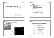
What you see of it 

Magnet (probe, sample) 

Console (transmitter, 

receiver, interface) 

Probe 

Computer (pulseprogramming, 

data processing) 


What you (usually) don't see of it 

1 Bore tube 

2 Filling port (N 2 

) 

3 Filling port (He) 

4 Outer housing 

5 Vacuum chambers/ 

radiation shields 

6 Nitrogen reservoir 

7 Vacuum valve 

8 Helium reservoir 

9 Magnet coil 

Inside a Magnet 


Tesla and MegaHertz 

The strength of a magnetic field is meassured in 

Tesla (for strong fields) or Gauss (for weaker 

fields). 1 Tesla corresponds to 10000 Gauss. The 

earth magnetic field is about 0.5 Gauss. 

The strength of an NMR magnet is usually given in 

terms of its 1 H resonance frequency in MHz: 

Tesla 2.3 8.4 11.7 14.1 16.5 17.6 21.1 

MHz 100 360 500 600 700 750 900 


Why go for stronger fields? 


Signal-To-Noise Ratio S/N 

S/N or the signal-to-noise ratio is a measure for the 

sensitivity of the NMR experiment: 

S/N ~ n γ 5/2 B 0 3/2 (NS) 1/2 T 2 T -1 

MHz 500 600 700 750 900 

S/N 1.0 1.3 1.7 1.8 2.4 

resolution 

1.0 1.2 1.4 1.5 1.8 

Relative sensitivity and resolution of our spectrometer 


Sensitivity Comes at a Price! 

~ €750.000 ~ €1.500.000 ~ €4.500.000 


Hardware (Summary) 

Magnet (Dewar, coil, shims) 

Probe 

Transmitter, receiver, amplifiers 

Acquisition computer (ADC) 

Sensitivity 


NMR VII 

NMR Parameters 

3 JHNHα (Hz) 

10 

9 

8 

7 

6 

5 

4 

3 

2 

1 

-150 -100 -50 0 50 100 150 

Φ(deg.) 


Parameters accessible by NMR 

Chemical shifts (resonance frequencies) 

Scalar coupling constants (Karplus, dihedral 

angles) 

Relaxation parameters (mobility, flexibility) 

Nuclear Overhauser Effect (interatomic 

distances) 

Chemical exchange (dynamic equilibria) 


Origin of Chemical Shifts 

B z 

The Larmor frequency (resonance 

frequency) is defined by the 

strength of the field B z and the 

gyromagnetic ratio of the nucleus: 

ω o = γ B z 


Origin of Chemical Shifts 

B z 

electrons 

(shielding) 

Shielding is 

proportional 

to external field: 

B loc 

B eff = B z + B loc 

nucleus 

= B z (1 – σ) 

B loc = -σ B z 


Local Fields - Local Frequencies 

With this new 'local' effective field 

B eff = B z + B loc = B z (1 – σ) 

we get a new 'local' Larmour frequency: 

ω i = γ B eff = γ ( 1 – σ i ) B z 


The Chemical Shift Parameter δ 

δ (ppm) = 10 6 (ν – ν ref ) / ν ref 

Difference in Hz divided by transmitter frequency 

The Chemical shift is a dimensionless parameter. 

Its values are given in parts per million, or ppm. 


Chemical Shift δ Frequency 

1 ppm ^= 

ν 0 / 10 6 Hz 

Example: At 600.13 MHz resonance frequency, 1 ppm 

corresponds to 600.13 Hz. 


Chemical Shift References 

References can be special substances which are 

added to the NMR sample, e.g. 

TMS (Tetramethylsilane) or 

TSP (Trimethylsilylpropionic acid) 

or the signal of the solvent (e.g. water) : 

δ H2O = 7.83 – (T[Kelvin]/96.9) 


Typical Chemical Shifts 

The range of chemical shifts observed depends on 

the sort of nuclei and the sort of molecules. In 

peptides and nucleic acids we typically find: 

1 

H: ~ 0 - 15 ppm 

13 

C: ~ 0 - 200 ppm 

15 

N: ~ 105 - 135 ppm 

Much smaller and bigger shifts can be observed in 

special cases! 


Chemical Shifts 

Usually: Classification of signals 

(identification of functional groups or local 

environment, aromatic, hydroxyl, amid 

protons) 

Peptides: In addition information about 

secondary structural elements 

(hydrogenbonds in loops, sheets and 

helices) 


A 1D-Spectrum of a Protein 

amide and aromatic 

protons 

H α – 

protons 

H β , H γ ,H δ ... 

(aliphatic) 

protons 


Chemical Shifts 

Usually: Classification of signals 

(identification of functional groups or local 

environment, aromatic, hydroxyl, amid 

protons) 

Peptides: In addition information about 

secondary structural elements (hydrogen 

bonds in loops, sheets and helices) 




Dispersion 

amide and aromatic 

protons 

H α – 

protons 

H β , H γ ,H δ ... 

(aliphatic) 

protons 


Typical 1 H Chemical Shifts 


Typical 13 13 C Chemical Shifts 


Less Signal than Nuclei: Chemical 

Equivalence 

Same chemical 

environment 

 

Same chemical 

shift value 

Nuclei in a symmetric situation or nuclei 

which 'feel' the same environment due to 

dynamical averaging (e.g. the protons of a 

methyl group) 


Chemical Equivalence 

H 

H 

C 

X 

X 

H 

H 

C 

C 

X 

X 

H 3 C 

X 

C 

X 

X 

All of of them are chemically equivalent, 

but for different reasons... 



H 

H 

C 

X 

X 

H 

H 

C 

C 

X 

X 

H 3 C 

X 

C 

X 

X 

Symmetry 

Dynamical 

averaging 



If we are able to see which nuclei in a 

molecule are equivalent, then we can tell 

how many different signals we expect in 

the spectrum of that molecule! 


Chemical Shift (Summary) 

Shielding of electron shell 

Local fields – local Larmor Frequencies 

Neighbours (bonds, H-bonds) 

References, ppm scale 

Dispersion 

Chemically equivalent nuclei 


Scalar Coupling 

(J-coupling, spin-spin coupling) 

Splitting of lines in NMR spectra (multiplets). 

Spin states of neighboring nuclei (mainly 1-3 

bonds away). 

Size : Number of bonds, kind of bonds, kind 

of neighbors and bond angles involved. 

Multiplicity : Depends on number of equivalent 

neighbors (n+1). 


Scalar Coupling (J-coupling) 

A 

B 

ν A 

ν B 

Two signals of nuclei with no J-coupling between them 


Scalar Coupling (J-coupling) 

J AB = 

AB coupling in in Hz Hz 

(is (is independent of of B 0 ) 

0 ) 

J AB 

J AB 

Bβ 

Bα 

Aβ 

Aα 

ν A 

ν B 

Two signals of nuclei with J-coupling between them 



(J-coupling) 

Scalar coupling only occurs between nonequivalent 

nuclei: 

If they are not chemically equivalent 

If they are chemically equivalent but not 

magnetically equivalent. 


Magnetic Equivalence 

If a set of chemically equivalent nuclei, a 

and b share the same coupling constant 

with every other nucleus in the molecule 

(e.g. x) they are magnetically equivalent : 

J ax = J bx and J ax' = J bx' 

H a 

H b 

X 

J ax = J bx 

J 

C 

C C 

ax ≠ J bx 

J ab = 0 J ab ≠ 0 

X' 

H a 

H b 

X 

X' 

magnetically equivalent magnetically not equivalent 


Common Coupling Multiplets 

singlet doublet triplet quartet pentet 


Multiplicity of Scalar Couplings 

The number of equivalent nuclei 

defines the number of possible 

spin-state combinations for a 

neighboring group : 







OH-group 

1 proton: 

α or β 

β 

α 

Energy level diagram 







CH 2 -group 

2 protons: 

ββ, 

αβ, βα, 

αα 

Energy level diagram 



CH 3 -group 

3 protons: 

βββ, 

αββ, βαβ, ββα, 

ααβ, αβα, βαα, 

ααα 






Energy level diagram


The number of multiplet-components depends 

on the number of different energy levels. The 

intensities of the multiplet-components can be 

derived from the number of equivalent spinstates: 







2 3 4 







1 

1 

1 

2 

1 

1 

3 

3 

1 


Common Coupling Multiplets 

β α 

αβ 

ββ αα 

βα 

ββα ααβ 

βαβ αβα 

αββ βαα 

Multiplet: 

βββ 

ααα 

Multiplicity: 

Intensities: 

Neighbors: 

singlet doublet triplet quartet pentet 

1:1 1:2:1 1:3:3:1 1:4:6:4:1 

non 1 2 3 4 



1 

1 1 

1 2 1 

1 3 3 1 

1 4 6 4 1 

1 5 10 10 5 1 

1 6 15 20 15 6 1 

. . . . . . . . . . . . 

The Pascal triangle 


Schematic Spectrum of CH 3 CH 2 OH 

(shifts only) 

OH CH 2 CH 3 

The integrals of the signals are proportional 

to the number of protons they represent 


Schematic Spectrum of CH 3 CH 2 OH 

with coupling 

OH CH 2 CH 3 

The integrals of the signals are still proportional 

to the number of protons they represent 


Real Spectrum of CH 3 CH 2 OH 

'with coupling' 

1 

H NMR spectrum of ethanol 

(Arnold et al., 1951) 


Real Spectrum of CH 3 CH 2 OH 

with coupling 

OH CH 2 CH 3 


Use of Scalar Couplings 

The scalar coupling between neighboring 

atoms can not only be used to identify 

neighbors in the molecule, they also, as we 

will see later, contain valuable structural 

information! 


Scalar Coupling (Summary) 

Effect via bonds to neighboring nuclei. 

Results in splitting of NMR lines. 

Origin: Different spin state combinations of 

neighboring nuclei. 

Depends on: Number of bonds, kind of bonds, 

kind of neighbors and on bond angles involved. 

Multiplicity depends on the number of 

equivalent neighbors (n+1). 


Relaxationrates 

Information about the association state of 

a molecule (monomeric, dimeric, …) 

Information about the shape of a molecule 

(anisotropic relaxation behaviour) 

Information about local dynamic/flexibility 

(e.g. binding sites in complexes, linkers of 

domains) 


NMR VIII 

The Nuclear Overhauser Effect 

A 

B 

RF 

RF 

RF 


Nuclear Overhauser Effect 

Dipolar cross-relaxation 

Intensity of one nucleus has influence on 

intensity of another 



A 

B 

regular spectrum 

RF 

NOE, small molecule 

RF 

RF 

NOE, large molecule 



(M − M 

η = 

M 

eq 

eq 

) 

η describes the change in intensity of 

a signal due to the NOE 


Energy Level Diagram 

W 1A 

ββ 

W 2 

W 1B 

With population differences 

for the A and B transitions 

in the undisturbed system: 

αβ 

βα 

A 0 = B 0 = Δ 

W 0 

W 1B 

W 1A 

W 0 and W 2 involve simultaneous 

transitions of spins A 

and B. 

αα 



A = 1.5 Δ 

A 

W 2 > W 0 

W 1A 

A 

W 2 

small molecules 

A 

W 1B 

W 1B 

W 1A 

W 0 

A 

W 0 > W 2 

large molecules 

A 

A 0 = B 0 = Δ 

A = A 0 = Δ 

B = 0 

A 

A = 0.5 Δ 



In practice we find the NOE ranging from +0.5 for 

small up to -1.0 for large molecules: 

η 

0.5 

0.0 

-0.5 

-1.0 

0.01 0.1 1.0 10 100 

fast 

tumbling 

ω o τ c 

slow 

tumbling 


Distances from NOEs 

η ~ 

τ c 

r 6 

τ c = rotational correlation time (size of molecule) 

r = distance between the two corresponding atoms 


Distances from NOEs 

η 

η ref 

τ c 

r 6 

= 

τc 

ref . r6 ref 

⇒ 

r = r ref 

6 

η ref 

η 

τ c ≈τ c 

ref 


Application for NOEs 

Information about short 1 H- 1 H-distances in 

molecules (< 5Å) 

Translated into distance-constraints 

applied in Molecular Simulations 

Main source of structural information in 

NMR 


Short 1 H- 1 H Distances in Proteins 


Nuclear Overhauser Effect (Summary) 

Dipolar Cross Relaxation 

Through space (< 5Å) 

Depends on size/mobility of molecule 

#1 source of structural information 

Reference distance necessary for 

translation into distances 


NMR IX 

Relaxation Measurements 

+1 

M z 

τ 

-1 

τ = ln(2)T 1 

τ >> T 1 


Relaxation (Reminder) 

T 1 : Longitudinal or spin-lattice relaxation. M z is 

restored, the system goes back to equilibrium. 

T 2 : Transverse or spin-spin relaxation. 

Transversal magnetization M x,y vanishes, the 

observable signal disappears. 


T 1 -Measurement 

180 o 90 o τ = 0 

τ 

Inversion recorvery 

τ = ln(2)T 1 

M z z 

(τ)=M o o 

[1-2exp(-τ/T 11 )] )] 

τ >> T 1 


Inversion Recovery 

τ 

M z z 

(τ)=M o o 

[1-2exp(-τ/T 11 )] )] 


Inversion Recovery 

M z 

+1 

0 

τ 

-1 

τ = ln(2)T 1 

τ >> T 1 

M z z 

(τ)=M o o 

[1-2exp(-τ/T 11 )] )] 


Fast T 1 -Measurement 

180 o 90 o 

τ 

τ = ln(2)T 1 

Inversion recorvery 

zero observable signal 

For a quick estimation of T 1 : directly search for the 

time τ, which gives us zero intensity (τ zero ) and 

calculate T 1 from this: 

T 11 = τ zero zero 

/ln(2) 



In principle we could calculate T 2 according to 

Δν 1/2 = 1/πT 2 

from the width of the Lorentzian lineshape of 

the signals in our spectrum. But... 

This value is strongly dependend from the 

inhomogeneity of our B 0 -field. 

We are rather interested in the 'pure' spinspin 

relaxation component (which, in contrast to 

the B 0 -field, is a molecular property)! 



90 o τ/2 

180 o 

τ/2 

T 2 

Spin-echo sequence 

I(τ)=I(0)exp(-τ/T 2 )] )] 



90 o 180 o 

τ/2 τ/2 T 2 

Spin-echo sequence 

Before 

acquisition 

Before 90 o 

After 90 o 

Before 180 o 

After 180 o 



The spin-echo experiment: 

Compensates for the component of T 2 that 

origins from field inhomogeneity 

The relaxation induced by dipolar spin-spin 

interaction can be measured selectively 

Important dynamic properties of the 

molecule can be extracted that way 



The experiment is repeated a number of 

times with increasing delays τ. 

T 2 is obtained from a plot of ln[ I (τ) ] 

against τ: 

ln[I (τ) ] 

I (0) 

I I (τ)=I (τ)=I(0)exp(-τ/T 2 )] 

2 )] 

τ 


Relaxation Measurements (Summary) 

Inversion recovery (T 1 ) 

Fast T 1 determination 

Spin echo experiment (T 2 ) 

Separation of contributions to T 2 from 

static field inhomogeneities and 

molecular properties (dynamic) 


NMR X 

Two-Dimensional NMR 


1-Dimensional 

NMR 

1D FT-NMR 

(simplest case) 

preparation - detection 

S(t) 

FT 

S(ω) 




2-dimensional NMR 

2D FT-NMR 

S(t 1 ,t 2 ) 

FT 1 , FT 2 

S(ω 1 ,ω 2 ) 

t 1 

t m 

t 2 

Preparation - evolution - mixing - detection 




A Signal of a 2D Spectrum 


Contour plot of the same Signal 

Compare: Topographical map (lines of equal height) 


The Second Time Domain 

FT (t 2 ) 

The size of the 

signal depends on 

the evolution in t 1 : 

the signal is said to 

be 'modulated' 

with ω 1 

t 2 =0 

t 2 

t 1 

For simplicity we look at a single frequency ω 

which is the same in t 1 and in t 2 (no mixing)! 


The Second Time Domain 

FT (t 2 ) 

ω 2 

ω 1 

t 2 =0 

t 2 t 1 

FT (t 1 ) 


Raw Data of a Real Spectrum 



Real Data after FT of t 2


Real Data after FT of t 1

...and after FT of t 1 and t 2 

Diagonal peaks 

Cross peaks 


The Mixingperiod 

t 1 

t m 

t 2 

Preparation - evolution - mixing - detection 

In the mixing period the frequency modulation 

of one nucleus is transferred to another one! 


The Mixingperiod 

No mixing (τ m = 0): Only diagonal peaks! 

Mixing (τ m > 0): We get cross correlated 

peaks (cross peaks)! 


The Mixingprocess 

Partial transfer 

Complete transfer 


Some 2D Experiments 

Depending on the experiment (pulse sequence) the cross 

peaks in a 2D spectrum show correlations based on 

different effects: 

• SCOTCH: light induced chemical exchange. 

• NOESY: cross-relaxation (spatial proximity) or exchange. 

• COSY: J-coupling (through bond connectivities of 

neighboring atoms, max. ~3 bonds). 

• TOCSY: J-coupling (through bond connectivities of 

neighboring atoms, >3 bonds in multiple steps). 

• HETCOR: 1 J-coupling, correlation of a proton and the 

heteronucleus (e.g. 15 N or 13 C) it is bound to. 


The SCOTCH Experiment 

Spin COherence Transfer in (photo) CHemical reactions 

hν 

Reaction A B with a proton at ω A in A which 

resonates at ω B in B. 

t 1 l 

i 

g 

h 

t 

t 2 

The corresponding pulse sequence 



t 1 l 

i 

g 

h 

t 

t 2 

The proton's magnetization is in t 1 

modulated with the frequency ω A . 

After the light pulse, the same 

proton evolves with ω B . 

Subsequent FT of the both 

time domains results in a 

2D spectrum with a peak at 

ω A in F 1 and ω B in F 2 : 



t 1 l 

i 

g 

h 

t 

t 2 

The proton's magnetization is in t 1 

modulated with the frequency ω A . 

After the light pulse, the same 

proton evolves with ω B . 

If A would not completely be 

converted to B by the light 

pulse, we would be able to 

observe a diagonal peak of 

A as well: 


2D NOE Spectroscopy (NOESY) 

t 1 

t m 

t 2 

C 

H B 

C 

C 

C 

B 

A 

H A 

H C 

A 

B 

C 

d HA-HB 

= d HC-HB 

> 5Å 

d HA-HC 

< 5Å 

NOESY: spatial proximity of 

nulei (distance < 5Å) 


J-correlated Spectroscopy 

(COSY and TOCSY) 

C 

C 

B 

Spinsystem 

B 

A 

B 

A 

COSY: J-coupling (through 

bond connectivities of neighboring 

atoms, max. ~3 bonds) 

C 

A 

B 

C 

A 

TOCSY: J-coupling (through 


atoms, >3 bonds) 


COSY and TOCSY 

t 1 

t 2 

t 1 mixing t 2 

COSY: J-coupling (through 


atoms, max. ~3 bonds) 

TOCSY: J-coupling (through 


atoms, >3 bonds) 

Multi-step transfer: each single 

step limited to max. ~3 bonds 

(like in COSY)! 


Two Examples: Alanine and Valine 

O: COSY X: TOCSY +: NOESY 


2D Spectroscopy (Summary) 

‘Indirect’ evolution time, t 1 

Mixing (dependent on experiment) 

SCOTCH (light induced) 

Complete/incomplete transfer 

NOESY (dipolar cross relaxation) 

COSY, TOCSY (J-coupling) 


NMR XI 

Spectral Assignment 


2D 1 H- 1 H NOESY of a Protein 


The Assignment Problem 

In order to be able to interpret NMR data, 

we have to know which signal (peak) in the 

NMR spectrum corresponds to which atom in 

the molecule. The process of determining 

this correlation is called 'assignment'. 


Information useful for Assignment 

Chemical shift: What is the surrounding of a 

nucleus (functional group, aromatic)? 

J-coupling: Which peaks (multiplets) belong 

together (neighbouring nuclei)? Familiar patterns 

(ethyl- or ethoxy group). 

Signal intensities: Integrals give information 

about number of equivalent nuclei. 

NOE data: Where are corresponding distances 

in the molecule? Connection of spin-systems. 


An Example: Ethylbenzene 


1 H Spectrum of Ethylbenzene 

3 

5 2 


13 13 C Spectrum of Ethylbenzene 

2 

2 

CDCl 3 

1 

1 

1 

1 


APT Spectrum of Ethylbenzene 

Attached Proton Test: 

CH 0 and CH 2 : negative 

C H and CH 3 : positive 


COSY Spectrum of Ethylbenzene 


HETCOR Spectrum of Ethylbenzene 



From the QM practical

From the QM practical (zoomed in) 

ortho (1,2) meta (1,3) para (1,4) 


Identification of Amino Acids 



Assignment (Summary) 

Finding pairs: signals atoms 

Shifts 

J-coupling 

Integrals 

NOEs 

Compare with known structure 

Identify spin system ‘patterns’ (e.g. 

amino acids) 


Weet je het nog...? 

B z 

B loc 

I z = hm I 

μ z = γ hm I 

E = - μ•B 

B eff = B z + B loc 

= B z (1 – σ) 

δ (ppm) = 10 6 (ν – ν ref ) / ν ref 


Weet je het nog...? 

NOE 

M y 

1 

FID 

0 

-1 

t 

Spin-echo 

sequence (T2) 

Inversion 

Recovery (T1) 

2x FT 

S(t 1 ,t 2 ) S(ω 1 ,ω 2 ) 

2D 

t 1 

t m 

t 2 


r = r ref 

6 

COSY/TOCSY 

NOESY 

η ref 

η

NMR XII 

Biomolecular NMR 



Bio(macro)molecules

Peptides and Proteins 

Peptides and proteins are 

mainly build from 20 

different naturally 

occuring amino acids. They 

all share the same basic 

structure and only differ 

in their side chain R. 


Amino Acids (general structure) 

Amino group 

H α 

| O 

H 2 N C α C 

Carboxyl group 

| OH 

R 

Side chain 


The Peptide Bond 

In peptides, amino acids are linked via a so-called 

peptide bond. The amino group of one residue is 

connected with the carboxyl group of another: 

H 

| 

H 2 N C a 

| 

R 

C 

O 

OH + 

-H 2 O 

H 

| 

H 2 N C a 

| 

R 

C 

O 

OH 


The Peptide Bond 

In peptides, amino acids are linked via a so-called 

peptide bond. The amino group of one residue is 

connected with the carboxyl group of another: 

H 

| 

H 2 N C a 

| 

R 

C 

O 

H 

| 

N C a 

| | 

H R 

C 

O 

OH 

Note: The peptide bond is planar due 

to its partial double bond character! 


Amino Acids 

Amino acids are usually referred to with either a oneletter 

or a three-letter code: 

Glycine Gly G Histidine His H 

Alanine Ala A Proline Pro P 

Valine Val V Aspartate Asp D 

Leucine Leu L Glutamate Glu E 

Isoleucine Ile I Asparagine Asn N 

Serine Ser S Glutamine Gln Q 

Threonine Thr T Lysine Lys K 

Phenylalanine Phe F Arginine Arg R 

Tyrosine Tyr Y Cysteine Cys C 

Tryptophane Trp W Methionine Met M 


Properties of Amino Acids 

+ - p h c a 

G * * 

A * * 

V * * 

L * * * 

I * * 

S * 

T * * 

F * * 

Y * * * 

W * * * 

+ - p h c a 

H * * * 

P 

D * 

E * 

N * 

Q * 

K * 

R * * 

C * 

M * 

+: positive, -: negative, p: polar, h: hydrophobic, c: aliphatic, a: aromatic 


Random Coil 1H 1H Chemical Shifts of of Amino Acids 

NH Hα Hβ 

G 8.39 3.97 

A 8.25 4.35 1.39 

V 8.44 4.18 2.13 CH 3 0.97 0.94 

L 8.42 4.38 1.65 Hγ 1.64 

CH 3 0.94 0.90 

1.19 

I 8.19 4.23 1.90 CH 2 1.48 

CH 3 0.89 

CH 3 0.95 

T 8.24 4.35 4.22 CH 3 

F 8.23 4.66 3.22 

2.99 

Y 8.18 4.60 3.13 

2.92 

P 4.44 2.28 

2.02 

C 8.31 4.69 3.28 

2.96 

S 8.38 4.50 3.88 

M 8.42 4.52 2.15 

2.01 

H2,6 

H3,5 

H4 

H2,6 

H3,5 

1.23 

7.30 

7.39 

7.34 

7.15 

6.86 

γCH 2 2.03 

δCH 2 3.68 

3.65 

γCH 2 2.64 

εCH 3 2.13 

NH Hα Hβ 

H 8.41 4.63 3.26 

3.20 

W 8.09 4.70 3.32 

2.99 

D 8.41 4.76 2.84 

2.75 

E 8.37 4.29 2.09 

1.97 

N 8.75 4.75 2.83 

2.75 

Q 8.41 4.37 2.13 

2.01 

K 8.41 4.36 1.85 

1.76 

R 8.27 4.38 1.89 

1.79 

H2 

H4 

H2 

H4 

H5 

H6 

H7 

NH 

γCH 2 

NH 2 

8.12 

7.14 

7.24 

7.65 

7.17 

7.24 

7.50 

10.2 

2.31 

2.28 

7.59 

6.91 

2.38 

6.87 

1.45 

1.70 

3.02 

7.52 

1.70 

3.32 

7.17 

CH 2 

NH 2 7.59 

γCH 2 

δCH 2 

εCH 2 

+ 

NH 3 

γCH 2 

δCH 2 

NH 6.62 

For X in GGXA, pH 7, 35ºC (Bundi and Wüthrich 1979) 


Assignment of Biomacromolecules 

Repetition of the same sort of spin systems 

Restricted set of monomers 

Simplifies the assignment of building blocks 

Complicates sequential assignment 

Isolated spin systems --> no J between aa’s 


Assignment, , Step by Step 

1. Spin-system Identification 

Characteristic shifts and patterns in COSY and 

TOCSY --> types of nucleotides or amino acids. 

2. Sequential Assignment 

Connection of spin-systems with sequential NOEs. 

3. Matching the Sequence 

Matching stretches with the known sequence. 


Classical Sequential Assignment 

J-coupling 

NOE 

J-coupling 


The Classical Sequential Assignment 

Method 

Combination of homo-nuclear 2D experiments 

which give correlations via bonds (COSY-type 

experiments) and others which give 

correlations through space (NOESY-type 

experiments). 

(Method of Wüthrich) 


Two Examples: Alanine and Valine 



AA Spin Systems 

Gly: Two H α s 

Pro: No amide proton (NH) 

Trp: NH at ~10ppm 

Ser, Thr: H α and H β very close together 

Aromatic sc: additional signal next to NHs 

NH sc: additional signal next to NHs 

NH 2 sc: additional signal between NHs and H 2 O 

Aliphatic sc: right half of spectrum (usually right 

of H α s) 


NOEs and NOE Combinations 

Distance (Å) (j - i = 1) (%) 

d αN 

(i,j) ≤ 2.4 

≤ 3.0 

≤ 3.6 

d NN 

(i,j) ≤ 2.4 

≤ 3.0 

≤ 3.6 

d βN 

(i,j) ≤ 2.4 

≤ 3.0 

≤ 3.6 

98 

88 

72 

94 

88 

76 

79 

76 

66 

d αN 

(i,j) ≤ 3.6 && d NN 

(i,j) ≤ 3.0 99 

d aN 

(i,j) ≤ 3.6 && d βN 

(i,j) ≤ 3.4 95 

d NN 

(i,j) ≤ 3.0 && d βN 

(i,j) ≤ 3.0 90 


Peptides (Summary) 

20 amino acids 

Peptide bonds 

Classification of side chains 

No J-coupling over peptide bond (H,H) 

Assignment (Wüthrich): 

COSY/TOCSY for aa identification 

NOESY for sequential assignment 


NMR XIII 

Structure Determination 


Structural Elements in Peptides 

GMRALEQFANEFKVRRIKLGYTQTNVGEALAAVHGSEFSQTTICRF 

ENLQLSFKNACKLKAILSKWLEEAEQVGALYNEKVGANERKRKRRTT 

ISIAAKDALERHFGEHSKPSSQEIMRMAEELNLEKEVVRVWFCNRR 

QREKRVK 

PIT-1 

(Transcription Factor 

Pituitary-1) 

PDB entry: 1AU7a 

Primary structure 

(a.a. sequence) 

Secondary structure 

(helix, loop, sheet) 

x N 

Tertiary structure 

(overall fold) 

Quaternary structure 

(aggregation state) 


After the Assignment 

Collect structural information: 

NOE data (2D, 3D) 

J-couplings for dihedral angles 

H/D exchange data 

Conduct computer simulations 

Present a nice structure… 


Inter-atomic Distances 

Inter-atomic distances 

can be bonded or non-bonded 


NOE Data 

Non-bonded distances 

define secondary and 

tertiary structure 


NOE constraints 

Typically some thousand NOE peaks in 2D 

NOESY spectra from a protein of 

moderate size. 

Each peak can be converted into an interatomic 

distance. 

These distances are used as constraints in 

computer simulations. 


NOE constraints 

Inter-proton distances 

non-bonded,

Accuracy of NOE distances 

In principle very accurate distances can be 

calculated from NOEs. 

In practice relatively low precision: 

••variation in in τ c due to local motion 

• dynamical averaging 

• spin diffusion 


Spin Diffusion 

NOE 

NOE 

NOE 

H A H B H C H D 

NOEs can be be 'propagated' between 

protons relatively far from each other 


Ranges for NOE constraints 

Rather than using precise distances, NOEs are 

classified into distance ranges: 

strong NOE (1.8 – 2.7 Å) 

medium NOE (1.8 – 3.5 Å) 

weak NOE (1.8 – 5.0 Å) 


Sequential and Medium Range NOEs 


Anti-Parallel 

β-sheet 


Parallel β-sheet 


Short Distances in α - Helix 

The shortest distance in in a 

regular α-helix is is found 

between HN(i) and HN(i+1) 


NOEs and Secondary Structure 


NOEs (Summary) 

Most important structural data 

Averaging due to dynamics 

β-sheets: short HN – Hα distances 

α-helix: short HN – HN distances 





Spin states of neighboring nuclei (1-3 bonds 

away). 









Spin states of neighboring nuclei (1-3 bonds 

away). 






J-coupling constraints 

10 

9 

R 

CO 

N 

H 

θ 

H α 

3 JHNHα (Hz) 

8 

7 

6 

5 

4 

3 

2 

1 

-150 -100 -50 0 50 100 150 

Φ (deg.) 

Karplus: J = A cos cos 2 2 (θ) (θ) + B cos(θ) + C 



Most important backbone angle can be calculated 

from the J-coupling between H α and amide proton: 

Karplus: J HNHα HNHα 

= 6.51 cos 22 (θ-60) + 1.76 cos(θ-60) + 1.60 

Also this angle (like the distance constraints derived 

from NOE data) can be used as constraints in molecular 

simulations. 



Like with NOEs, also J-couplings may be only an 

average of different dynamic situations (conformational 

exchange). 

In addition the Karplus equation gives ambiguous 

results for different values of J. 

Most reliable are values of J HNHα of: 

9 – 10 Hz (for extented β-sheet structures) 

3 – 4 Hz (for α-helical structures) 

Values between 6 and 7 may reflect averaging! 


J-coupling (Summary) 

Karplus equation 

Averaging due to dynamics 

Extented β-sheet: 9 – 10 Hz 

α-helix: 3 – 4 Hz 


Structure Calculation 

The general steps: 

Create a (set of) starting structure(s) 

Optimization of the structure(s) 

(molecular dynamics simulation) 

Evaluation of resulting structures 

Selection of 'final' structure(s) 


The Starting Structure 

'Builder' user interface of the modelling 

program. 

In most cases the input of the sequence 

is sufficient to generate an 'extended' 

structure (basic geometry). 


Optimization of the Structure 

For the optimization of the structure the 

most common approach is: 

Restraint Molecular Dynamics (RMD) 

using Simulated Annealing (SA) 


Restrained Molecular Simulation 


Restrained Molecular Simulation 


Molecular Dynamics Simulation 

A Molecular Dynamics Simulation is a 

computer simulation (= calculation) of 

the movement of the atoms in a 

molecule. 


The Force Field 

The force F i is calculated from tabulated potentials 

(the force field) and the current position r i : 

F 

i 

= − 

∂V 

∂r 

i 

The empirical potential energy function V contains 

terms like: 

V 

= Vbondlength 

+ Vbondangle 

+ Vdihedral 

+ VvanderWaals 

+ Velectrostatic 

+⋅⋅⋅⋅ 


Potential Energy Function 

l 

E 

Potential Energy 

Function for 

Bond Length 

Bondstretching 

(vibrational motion) 

l 0 

l 


Newton's Equation of Motion 

Given initial coordinates and velocities, 

Newtons's equation of motion can be solved 

for all atoms i with the mass m i , position r i 

(a vector) and the Force F i (a vector, too), 

currently acting on the atom: 

m 

i 

d 

dt 

2 

r i 

2 = 

F 

i 


The Constraints 

In addition to potentials of force field: 

'Home-made' constraints for distances 

and/or bond angles (from our NMR data) 

Special additional potentials of various (user 

defined) shapes. 

Additional terms to the initial function V. 


NOE Constraints 

With the following terms we can add 

constraints for an upper (u ij ) and lower (l ij ) 

limit for the distance r ij : 

V 

NOE 

= k( 

r 

= 0 

ij 

− u 

ij 

) 

2 

if 

if 

r 

l 

ij 

ij 

> u 

≤ 

r 

ij 

ij 

< 

u 

ij 

= 

k( 

l 

ij 

− 

r 

ij 

) 

2 

if 

r 

ij 

< l 

ij 


NOE Constraints 

The actual shape of the potential may look 

like this: 


Molecular Dynamics 

Typical time scales for molecular motions are given 

in the following table: 

Time scale Amplitude Description 

short femto to pico 

10 -15 -10 -12 s 

medium pico to nano 

10 -12 -10 -9 s 

long nano to micro 

10 -9 -10 -6 s 

very long micro to second 

10 -6 -10 -1 s 

0.001 - 0.1 Å - bond stretching, angle bending 

- constraint dihedral motion 

0.1 - 10 Å - unhindered surface side chain motion 

- loop motion, collective motion 

1 - 100 Å - folding in small peptides 

- helix coil transition 

10 - 100 Å - protein folding 


Time Steps of the Simulation 

Fastest motions femto seconds 

Limitation of single steps of simulation to 

shortest 'events' 

Prevention of unproportional increase of 

forces (molecules could 'explode'!) 


Local or Global Energy minimum ? 

Structural landscape is filled 

with peaks and valleys. 

Minimization protocol always 

moves “down hill”. 

No means to “see” the overall 

structural landscape 

No means to pass through 

higher intermediate 

structures to get to a lower 

minima. 

The The initial initial structure determines the the results of of the the minimization! 


Simulated Annealing 

Often used with RMD 

Potentials are 'down-scaled' in the beginning 

Higher degree of freedom ('sampling a bigger 

conformational space') 

In later steps the potentials are slowly brought to 

their final values. 

This is like first heating up the molecule and then 

cooling it down in small steps. 


Family of Structures 

Usually a big number of calculations is done in parallel: 

Starting from a set of structures and ending in a family 

of structures, from which an average structure may be 

created or the one with the minimum energy may be 

selected. 

Family of structures 

of the protein crambin 


Final Published 3D Structures 

of 

Molecules 


Restrained Molecular Dynamics 

(Summary) 

Choosing a force-field. 

Add constraints from NMR data 

Starting coordinates of all atoms (starting structure). 

Starting velocities of all atoms ('random seed 

numbers', Maxwell Boltzmann distribution). 

Solving Newton's classical equation of motion for very 

small steps. 

Calculation of new coordinates, forces and 

velocities. 

Repeat steps 5 and 6 and find structure with 

minimum energy. 



The End

0 - NMR Spectroscopy Research Group

Create successful ePaper yourself

Delete template?

Save as template?