Depth of field and Scheimpflug's rule - Large Format Photography. Info

Depth of field and Scheimpflug’s rule : a “minimalist” geometrical approach
Emmanuel BIGLER
September 6, 2002
ENSMM, 26 chemin de l’Epitaphe, F-25030 Besancon cedex, FRANCE, e-mail : bigler@ens2m.fr
Abstract
We show here how pure geometrical considerations with an absolute minimum of algebra
will yield the solution for the position of slanted planes defining the limits of acceptable sharpness
(an approximation valid for distant objects) for Depth-of-Field (DOF) combined with
SCHEIMPFLUG’s rule. The problem of Depth-of-Focus is revisited using a similar approach.
General formulae for Depth-Of-Field (DOF) are given in appendix, valid in the close-up range.
The significance of the circle of least confusion, on which all DOF computations are based,
even in the case of a tilted view camera lens and the choice of possible numerical values are
also explained in detail in the appendix.
Introduction
We address here the question that immediately follows the application of SCHEIMPFLUG’s rule:
when a camera is properly focused for a pair of object/image conjugated slanted planes (satisfying
“SCHEIMPFLUG’s rules of 3 intersecting planes”), what is actually the volume in object space that
will be rendered sharp, given a certain criterion of acceptable sharpness in the (slanted) image/film
plane?
Again the reader interested in a comprehensive, rigorous, mathematical study based on the geometrical
approach of the circle of confusion should refer to Bob WHEELER’S work [1] or the
comprehensive review by Martin TAI [2]. A nice graphical explanation is presented by Leslie
STROEBEL in his reference book [5], but no details are given. We re-compute in the appendix
STROEBEL’S DOF curves and show how they are related to the classical DOF theory. The challenge
here is to try and reduce the question to the absolute minimum of maths required to derive a
practical rule.
It has been found that, with a minimum of simplifications and sensible approximations, the
solution can be understood as the image formation through the photographic lens fitted with
an additional positive or negative “close-up” lens of focal length ¢¡ , where ¡ is the hyperfocal
distance. This analogy yields an immediate solution to the problem of depth of field for distant
objects, the same solution as documented in Harold M. MERKLINGER’s work [3], [4], which
appears simply as an approximation of the rigorous model, valid for far distant objects.

1 Derivation of the position of slanted limit planes of acceptable
sharpness
1.1 Starting with reasonable approximations
Consider a situation where we are dealing with a pair of corresponding slanted object and image
planes according to SCHEIMPFLUG’s rule (fig. 4), and let us first assume a few reasonable
approximations:
1. first we neglect the fact that the projection of a circular lens aperture on film, for a single, out
of focus point object, will actually be an ellipse and not a circle. This is well explained by
Bob WHEELER [1] who shows, after a complete rigorous calculation, that this approximation
is very reasonable in most practical conditions.
2. second we consider only far distant objects; in other words we are interested to know the
position of limit surfaces of sharpness far from the camera, i.e. distances or ¡ much greater
than the focal length ¢ . We’ll show that those surfaces in the limit case are actually planes,
the more rigorous shape of these surfaces for all object-to-camera distances can be found in
Bob WHEELER’s paper, in Leslie STROEBEL’s book [5], and here in the appendix.
3. finally we’ll represent the lens as a single positive lens element; in other words we neglect
the distance between the principal planes of the lens, which will not significantly change the
results for far distant objects, provided that we consider a quasi-symmetrical camera lens
(with the notable exception of telephoto lenses, this is how most view camera lenses are
designed).
1.2 A “hidden treasury” in classical depth-of-field formulae !
Let us restart, as a minimum of required algebra, with the well-know expressions for classical depth
of field distances, in fact the ones used in practice and mentioned in numerous books, formulae on
which are based the DOF engravings on classical manually focused lenses.
Consider an £¥¤ object perpendicular to the optical axis, ¡§¦ let ¡©¨ and the positions (measured
from the lens plane in ) of the planes of acceptable sharpness around a given position of the
¡ object .
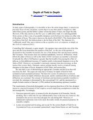
It should be noted (see fig. 1) that the ray tracing for a couple of points outside the optical
axis ¦ like ¦ and yields in the image £¤ plane an out-of-focus image of circular shape (not
an ellipse, as it could be considered at a first); this out-of-focus image is exactly the same as the
circular spot originated ¦ from ; this is simply the classical property of the conical projection of
a circular aperture between two parallel planes. The out-of-focus spot near is centred on the
median ¦ ¦ ray that crosses the lens at its optical centre. This point will be important in
the discussion about transversal magnification factors for out-of-focus images.
2

Figure 1: Depth-of-field distances ¦ , ¡ ¦ and ¨ , ¡©¨ for a given circle of confusion ¡
¢
¤
¢
£
¢
£
¢
¡
¤
¢
¤
¡
¢
¤
¢
£
¢
¢
¢
£
¤
¢
¡
¢
¢
¨
¦
£
¢
¦
far plane
of acceptable
sharpness
P2
object
plane
s2
D
B
A
D1
p2
near plane
of acceptable
sharpness
P1
s
s1
p
F
f
p1
lens plane
I
O
p’
f
F’
focal
plane
s’
D’ D’1
A’
B’
film
plane
circle of
confusion
c
Assuming a given value for , the diameter of the circle of confusion, ¡ ¦ and ¡©¨ are identical
whether we consider ¡ on-axis or off-axis and is given, for far distant objects, by
££
¢
¥ ¡
¢
(1)
¡
In eq.(1), ¡ is the hyperfocal distance for a given numerical aperture § and diameter of the
circle of confusion ¡ , defined as usual as
¡ ¦
¡©¨
£ ¢©¨ ¢
¡
¡ §¨
The previous expressions of eq. (1) are valid only for far-distant objects; readers interested by
more exact expressions, valid also for close-up situations, will find them below in the appendix.
Now let us combine eq.(1) with the well-known object-image equation (known in France as
DESCARTES formulae), written here with positive values ¡ of ¡ and (the photographic case)
£ ¢
§ ¡ (2)
(3)
Combining equation (1) into (3) yields the interesting formula (4)
¡
¢
¥ ¡
¢
(4)
¡
¢
¢
¡ ¦
¡
¡©¨
¡
3

¢
¢
¤
¦
¢
¢
¦
¢
¢
¤
which is nothing but the object-image equation for the image £ located at a distance ¡ of
the lens centre , but as seen through an optical system of inverse focal length
¢
¢
for ¡
the near plane ¡ ¦ (point ¦ ) and
¢
for the distant plane ¡ ¨ (point ¨ ). The expression
¡
¢
¢
¢
¡
is simply the inverse
of the focal length of a compound system made of the
¦ ¢
original lens, fitted with a positive close-up lens of focal length .
When you “glue” two thin single lens elements together into a thin compound with no air space,
¡
their convergences (inverse of the focal length) should simply be added. Thus in a symmetric way
¢
¢
¡
is nothing but the inverse
¨ ¢
original lens, fitted with a negative “close-up” lens of focal ¦
¡
length
of the focal length of a compound system made of the
.
1.3 A positive or negative “close-up” lens to visualise DOF at full aperture?
1.3.1 a classical DOF rule revisited
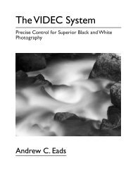
Before we proceed to the SCHEIMPFLUG case, let us examine the practical consequence of the
additional close-up lens approach in the simple case of parallel object and image planes. We’ll
show how this additional lens element will allow us to revisit some well-know DOF rules (figure 2).
It is known to photographers that when a lens is focused on the hyperfocal distance , all
objects ¡
located between and infinity will be rendered approximately sharp on film, i.e. sharp
within the DOF tolerance. Consider a lens focused on the hyperfocal distance and let us add ¡ £¢
a
¡
positive close-up lens element of focal length . The ray tracing on figure 2 shows that the
object plane located at a distance is now imaged sharp on film if the lens to film distance
is unchanged. In a symmetric way, the same photographic lens fitted with a negative “close-up”
¤
¡ ¤¢
additional lens element ¦
¡
of focal length will focus a sharp image on film for objects located at
infinity. The same considerations actually apply whatever the object to lens distance might be, in
this case formulae (4) are simply a more general rule valid for any object ¡ to lens distance ; the
result is eventually the same, i.e. the positions ¡ ¦ of ¡©¨ acceptable sharpness and are located where
the film “would see sharp” through the camera lens fitted with a positive or a negative “close-up”
¡
lens of focal ¦
¡
length or .
¤
1.3.2 DOF visualisation at full aperture??
¤ ¡
¦
¡
It would be nice to be able to use this trick in practice to check for depth of field without stopping
the lens down to a small aperture. In large format photography, f/16 to f/64 are common, and the
brightness of the image is poor; it is difficult to evaluate DOF visually in these conditions. The
close-up lens trick would, in theory, allow to visualise the positions of limit planes of acceptable
sharpness at full aperture simply by swapping a or supplementary lens by hand in front
of the camera lens with the f-stop kept wide open.
4

plane of sharpness
now located at H/2
lens
plane
f
initial object plane
located at the
hyperfocal distance H
A
a positive close−up lens
of focal length +H
is added
H/2
O
p’
F’
focal
plane
A’
H
with a close−up lens
of positive power, +H,
a film placed in A’
"sees" sharp at a distance H/2
sharpness plane
located at infinity
lens
plane
I
f
initial object plane
located at the
hyperfocal distance H
A
a negative "close−up" lens
of focal length −H
is added
O
p’
F’
focal
plane
A’
H
with a "close−up" lens
of negative power −H,
a film placed in A’
"sees" sharp at infinity
Figure 2: When the an additional “close-up” lens of positive or negative power +H or -H allows us
to find well-know DOF rules
5

¨
There is no reason why this could not work from an optical point of view. Unfortunately
classical close-up lenses are always positive and, to the best of my knowledge, my favourite opticist
round the corner will not have in stock eyeglasses with a focal length longer than 2 metres (a power
smaller than 0.5 dioptre). The shop will probably have all kinds of positive and negative lenses in
stock, but none, even on special order, will exhibit, say, a focal length of 10 metres (1/10 dioptre)
because this is quite useless for correcting eyesight.
In large format photography, the hyperfocal distance is always greater than 2 metres. For example
a large format lens, with a focal length of 150 mm, for which we consider appropriate a circle
of confusion of 100 microns has an hyperfocal distance smaller that 2 metres only when closed
down at a f-stop smaller than f/112. An impossible aperture, and moreover for such “pinhole” kind
of values, diffraction effects make the classical DOF model questionable.
Let us however see if this could work in 35mm photography. Shift and tilt lenses do exist for
35mm SLR cameras. Consider a moderate wide-angle of 35 mm focal length and assume that
the circle of confusion is chosen equal to the conventional and widely used value of 33 microns.
The hyperfocal distance is equal to 2 metres at f/18: this is a more realistic value. Those who use
shift and tilt lenses, 35mm focal length on a 35mm SLR can actually use a +0.5 or -0.5 dioptre
supplementary lens to get an idea of the DOF planes at f/16-f/22 without actually stopping down
the lens. And we’ll show below that this will be useful also for moderate tilt angles.
For large format photographers, actually the majority of users of tilts and shifts, the trick of
a positive or negative “close-up” lens will only be a very simple geometrical help to determine
where the slanted planes of acceptable sharpness in object space are located, as explained now.
1.4 Where Mr. Scheimpflug helps us again and gives the solution
When the film plane is tilted, the ray tracing is similar to the one on figs.1 and 2, but the object
plane is slanted (figures 3 and 4). We show now that even in this case, we can also consider
the camera lens fitted with a positive or negative close-up lens to determine the object planes of
acceptable sharpness.
1.4.1 a last argumentation without analytical calculations...
Now a subtle question that arises is: we now have the formula connecting the longitudinal position
of out-of-focus pseudo-images (actually: elliptical patches, close to a circle, when the tilt angle
is small) in the slanted film plane with the corresponding longitudinal position of a point source
in the object space. But what is the transversal magnification factor? To find this we need an
additional diagram (figure 3).
Due to basic properties of a geometrical projection of centre , if we neglect the “ellipticity”
of the DOF spot, the centre of the out-of-focus £ ¨ image, , is aligned with the median £¥¨ £ ¨ ray .
Hence, the transversal magnification factor for an out-of-focus £ image is the same as a for
a true image £ ¨ when is formed “sharp” through a compound lens fabricated by adding a thin
6

p2
p
p’
lens
plane
object plane
slanted film plane
farDOF limit
O A2’ A2" spot size
A2
**if the ellipse effect is neglected**
(small tilt angle)
the centre of the projected spot A2"
is aligned with A2 O A2’
Figure 3: The transversal magnification factor for an out-of-focus pseudo-image, ¡ ¡©¨ , is the same
as for a true image through a compound lens
supplementary lens to the camera lens. This transversal magnification factor (see fig. 3) is equal to
¡ ¨ , the same value would be obtained for £ ¨ as a true image through the compound lens.
¡
So both in longitudinal and transversal position the correspondence between the object space
and the image space for out-of-focus images is exactly the same as if viewed “sharp” through the
compound lens. Applying basic rules of true object-image formation we already know that the
image of a slanted plane is another slanted plane, we do not need any analytical proof to derive
what follows.
1.4.2 ...and Mr. Scheimpflug gives us the solution without any calculation!!
¢ ¦ ¡ ¦ ¢ ¨ ¡©¨
¦ ¦ ¨ ¨ ¡ £¢¡
¡ £¥
¡ ¦ ¦ ¡©¨ ¨
¨ £¥¤¨ ¨ £¡ ¤ ¦ £¥ ¦ ¡ ¦
¤
£
£¡ ¤§¦
¤©¨
As a consequence, without any further calculations we apply SCHEIMPFLUG’s rule to the compound
optical system and we conclude that the limit surfaces of acceptable sharpness for distant
objects are the slanted conjugate planes of the film plane with respect to a compound,
thin lens centred in , with a focal length equal to (for ) or (for ), and that all
those planes and intersect together in with the slanted object plane and the
slanted SCHEIMPFLUG-conjugated image plane as on fig.4.
To actually define where those planes are located, we simply have to impose that they should
cut the optical axis at a distance (point ) or (point ), respectively. Then, simple geometric
considerations on homothetic triangles vs. as well as vs. combined
with eq.1 yield the interesting and most simple final result: with , both distances and
are equal to
¤©¨ £
¤ ¦ £
¤
¡
(5)
¡
Now consider a plane ¦¥ ¦ ¨ perpendicular to the optical axis and located at the hyperfocal
7

G 1
h
hyperfocal distance
H
G
h
p
G 2 B 1
h f
P 1
2 P
A 1
F O F’
h C 2
C’
A’
B 2
approx
not valid
here
h
p 2
p 1
S
Figure 4: Position of slanted planes of acceptable sharpness, for distant objects, according to this
simplest model: fit the original lens with “close-up” lenses of focal length ( ¢¡
8

¢
¤
¢
¢
¥
¢
¤
¢
¢
¡
¡ £ © ¢
¤
vs. , we eventually get
¦ ¦ £
¦ ¨ £
¤ (6)
a nice result given by Harold M. MERKLINGER in ref.[4]. Note that for far distant objects,
the image point £ on the optical axis is located very close to the image focal point ; thus the
distance ¤ , hard to estimate in practice, can be computed from the “camera triangle” ¡ £ from
the focal length ¢
¢£¦¥¨§
£ © ¥§
and the estimated tilt angle
¡
¡ £ as: ¢¤£¦¥¨§
. For small tilt angles
¡ ¡
£¡ £ , which eventually yields the same result as in reference [4], where the
£¡
diagram is drawn with a reference line perpendicular to the film plane (hence a instead of a
) instead of the lens plane like here.
2 Application to the problem of Depth-of-Focus
Another classical photographic problem is the determination of Depth-of-Focus. The question is:
for a given, fixed, object plane, what is the mechanical tolerance on film position in order to get a
good image, within certain acceptable tolerances? The following (figure 5) yields the solution, at
least to start with the case of an object plane perpendicular to the optical axis and an image plane
parallel to the object plane.
If ¡ denotes the film position for an ideally sharp image of an object plane at a distance ¡ , the
two acceptable limit film plane positions ¡ ¦ and ¡ ¨ are given by
¤ ¢ ¢
¥ ¡ ¨
£ ¡
¡
¦ ¢ ¢
(7)
¡
¦
£ ¡ ¡
In order to keep the derivation as simple as possible and keep the equivalence with a true
optical image formation valid, we need an additional but reasonable approximation, namely that
the hyperfocal distance is much greater that the focal length ¢ . This is what happens in most
cases and is argumented in the appendix. Within this approximation, it is found (see details in the
¡
appendix), not so surprisingly, that the limit ¡§¦ positions ¡©¨ and as defined above for the Depth-of-
Field problem are approximately the optical conjugates of the ¡ ¦ positions ¡ ¨ and of the Depth-of-
Focus problem through the photographic lens of focal ¢ length , as given by DESCARTES formula
©
¢
©
¢
(8)
Combining this eq.(8) with the transversal magnification formula ¡ ¦ ¡ or ¡ ¨ ¡ , still the same
for pseudo-images (the centre of out-of-focus light spots) as for real images, we find that in the
general case of a slanted object plane, for far distant objects (so that equation (1) is valid), the
limit positions for the image planes in the Depth-of-Focus problem are given by two slanted
¡ ¦
¡ ¦
¡©¨
¡ ¨
9

¨
B
lens
plane
focal
plane
image
plane
p’
object
plane
A
F
f
I f p’2
O
F’
A2’’
A’
p’1
c
circle of
confusion
p
B’
Figure 5: A ray tracing similar to the ones used in the Depth-of-Field problem yields the solution
of the Depth-of-Focus problem
planes, those slanted image planes of acceptable sharpness being the optical conjugates (through
the lens of focal length f) of the slanted object planes in the Depth-of-Field problem.
Hence, applying SCHEIMPFLUG’S rule, we conclude again that those slanted planes intersect
together at the same point S (see fig. 6)
Appendix : depth of field formulae also valid for close-up, reasonable
limits for the choice of the circle of confusion
Depth-of-Field formulae valid for close-up
it is not too difficult (although rather
perpendicular to the optical axis to derive more general formulae giving
From NEWTON’s object-image formulae ¨ £ ¢ ¨ ¢ £ ¢
lengthy) for an object £¤
the position ¡ ¦ and ¡©¨ of the planes of acceptable sharpness around a given position of the object ¡
(as measured from the lens plane, see fig.1).
Those exact formulae (9) and (10) are used in a html-javascript [7] and a downloadable spreadsheet
[8] on Henri Peyre’s French web site. Another derivation, strictly equivalent, is proposed by
Nicholas V. Sushkin [6] offering an in-line graph.
There is however a restriction: those formulae will be also valid for a thick compound lens
where the pupil planes are located not too far from the nodal planes identical to principal planes
10

slanted object plane
P2 A P1
C
p 2
p 1
limit image plane P’2, Depth−of−Focus
slanted image plane
limit image plane P’1, Depth−of−Focus
S
P1 and P’1 are optically conjugated through the camera lens of focal length f
same for P2 and P’2, when H >> f, and p >> f
Figure 6: For a slanted object £¡ plane located far from the lens, and when the hyperfocal distance
is much greater than the focal length, the image planes of acceptable ¡ ¦ sharpness ¡ ¨ and in
the Depth-of-Focus problem are the optical conjugates of the slanted Depth-of-Field object planes
¦ and ¡ ¨ through the camera lens
¡
F
O
A’
C’
11

¢
£
¡
¢
¤
¡
¢
¦ ¢ ¢
¡
¡ ¤
§ ¡ ¦ ¢
¢
£
¡
¢
¦
¡
¦ § ¡ ¦ ¢
¡
¢
¦ ¢ ¢
¡
¢
in air. This is the case obviously for a single lens element or a cemented doublet, but also for quasisymmetric
view camera lenses; however for asymmetric lenses or more generally speaking for a
lens where pupil planes are far from nodal planes, an extreme case being, for example, so-called
telecentric lenses, this classical depth-of-field approach is no longer valid. Another ray tracing
diagram has to be taken into account; of course depth-of-field will increase when stopping down
such a lens, but this will not be quantitatively described by equations (9) or (10).
Assuming a given value for ¡ , the diameter of the circle of confusion, a derivation not shown
here yields the following (and surprisingly simple) result, which is presented in a slightly different
but strictly equivalent form by Nicholas V. Sushkin on his web site [6]
(9)
these formulae can be also written as
¡ ¦
¥
¡©¨
¡
¡
¡¢
¡
(10)
where (see ¢ fig.1) is the focal length of the lens (here considered as a single, positive, thin lens
¡ element) the position (measured from the lens plane ) of the object £¥¤ plane , assumed to be
perpendicular to the optical axis.
¡ ¦ Then is the position of the near limit plane of sharpness ¡ ¨ and the position of the far limit
plane of sharpness. It should be noted in eqs.(9), that all ¡ distances ¡ ¦ , , ¡©¨ and are (positive)
distances measured with respect to the lens plane plane . Here, for a thin positive lens, is
identical to the principal planes. No problem with a thick compound lens if pupillar planes are
not too far from principal planes, re-starting from the single thin lens element you just have to
“separate” “virtually” the object side from the image side by a distance equal to the (positive of
negative) spacing between principal planes.
¡ ¦ £
¥ ¡©¨ £
Definition of the “true” hyperfocal distance
Let us first point out that there is a subtle difference in what appears as the “true” hyperfocal
distance when exact formulae are used. If one tries in (9) or (10) to find ¡
the proper distance for
which goes to infinity, the value
¤
¢ of is found instead of in the conventional approach.
¡©¨
In this case, the near limit of acceptable sharpness will ¡ ¡ £ §
¡ ¤ ¤¢
be . In practice as soon
¡ £¥¤§¦©¨
as is much greater ¢ than , the difference is not meaningful. It could be possible to re-write
equations (9) and (10) as a function ¡
of , but we eventually prefer to denote by hyperfocal
£¥¤§¦©¨ ¡
distance the well-accepted value £ ¢ ¢ ¡ ¡ since it naturally comes out of the computation, and as
§
it is referred to in many classical photographic books.
With this assumption on pupillar planes, the formulae given in eq.(9) are derived from NEW-
TON’s formulae within the only, non-restrictive, reasonable approximation that the circle of confusion
(in the range of 20 to 150 microns) is smaller than the diameter of the exit pupil ¢ § .
¡
12

Taking ¡¡ £¢
§ sounds reasonable. For example with ¢ £ ¢ ¢¤¢ mm, the aperture diameter
¢
¢
to be smaller than one millimetre, whereas conventional
¢¥¢
values for never exceed 0.5mm.
It is also possible to think again about the significance of the hyperfocal distance ¡
¡
£ ¢ § should be smaller than ¢
by reintroducing
the value of the lens aperture diameter, £ ¢ § . The following expression is
obtained: H/f = a/c, in other words the ratio between the hyperfocal distance and the focal
length is equal to the ratio between the lens aperture diameter and the circle of confusion . ¡
¢
In
most practical cases, is much greater ¡ than . Considering a limit case where could be close
¢ ¡
to , although acceptable from a geometrical point of view, would yield values for that are too
¡ ¢
big to be acceptable: for example if can be as big as , equivalent to ¡ ¡ ¢
¢ , the resultant
£
image quality will be terrible.
£¢
Let’s put in some numerical data to support this idea. Consider a standard ¡ focal ¢ length equal
(by conventional definition of a standard lens) to the diagonal of the image format; assume that the
format is square to simplify. The image size will be equal to 0.7f by 0.7f (diagonal size = 1.4 times
the horizontal or vertical size of the square). If we
¤¢ £ ¢ §
¢
§ assume that , the number of
equivalent image dots will be ¡ ¢ §¦
£ § £ ¢ ©¨
only both horizontally or vertically. Even ¨ ¨ at
¢
f/90, this yields a total number of image points smaller than 20,000 ( ¢¥ ¢ ¢¥
¨ )!!! Even
¢ £ §
¢
§ ¨
if this “un-sharp” out-of-focus image concerns only a small fraction of the whole image, such a
terrible image quality is clearly unacceptable.
Now that we have shown that it is necessary to limit the upper value for for image quality
reasons, this upper limit being somewhat arbitrary, lets us demonstrate that there is also an absolute,
unquestionable, minimum value for ¡ due to diffraction effects.
¡
This pure geometrical DOF approach is valid as long as diffraction effects are neglected. Considering
a value equal § to microns ( ¢¤¢ ¨ § ¨ , with £ ¢ ©¥
in the worst case) for a
¢
diffraction spot in the image plane, the other reasonable condition is § in microns § microns.
For example in medium 6x6cm format with ¡ £ ¢
m, f/32 is a reasonable f-stop whereas f/64 is
irrelevant to the present purely geometrical approach. In 4”x5” format taking ¡ £ ¢ ¢
m, f/128
¡
will be the smallest non-diffractive aperture for depth-of-field computations.
In macro work at 1:1 ratio (2f-2f), DOF does not depend on the focal length
With all above-mentioned assumptions, equation (9) is valid even for short ¡ distances as in macro
work, ¡ ¢ with of course to get a real image. This will be in fact irrelevant to our purpose to
find a simple expression and graphical interpretation for far-distant objects, but is of practical use
in macro- and micro-photography. For example ¡ £ ¢
¢ when at 1:1 magnification ratio, the total
depth of field is given by ¡ ¨ ¦ ¡ ¦ £ ¨
well-know result.
§ ¡
, and is totally independent from the focal length, a
13

¢
¢
¤
¤
¢
¢
£
£
¢
¢
¢
¢
¦
¢ ¢
¡
¦
¢ ¢
¡
¢
¢
¢
¡
§
¡
¦ ¢
¨
¨
¨
¢
A numerical computation in agreement with Stroebel’s diagrams
Unfortunately there is probably nothing really simple in terms of understanding geometrically
depth-of-field zones for close-up when the film plane is tilted at a high angle with respect to the
optical axis.
From eq.(9) we easily derive a limit form valid for far distant objects, ¡ i.e. much greater than
yields the well-known expressions of eq.(2).
and ¦ ¢
¡
¢
i.e. ¡ ¢ . In this case we can write that ¢ ¡£¢
¢
To go a little further, a numerical computation and graphical computer plot (fig.7) is required.
However it is interesting to find the origin of the diagram presented in STROEBEL’s excellent
reference book [5], stating that limit planes of acceptable sharpness intersect all in the same pivot
¤¦¥ point located not in the lens plane (like in our approximate model here) but also in the slanted
object £ ¡ plane , and one focal length ahead of the “regular” Scheimpflug’s pivot § point (figure 7).
© ¢
, ¡ £¥¤§¦©¨ £ ¡ ¤
¢
©
¢ . This
Without any calculation ¡ when decreases down to the limit ¡ £ ¢ value , it is easy to see from
eq.(9) that both ¡ ¦ values ¡©¨ and become equal ¢ to this defining the pivot point Pf.
From the computed diagram, here plotted the particular value of ¡ £ ¢
¢¤¢¤¢ ¢ ¢ ¦ ¢ ( ¢
is mentioned sometimes and is more stringent), the simplified approach of the “plus or minus H”
close-up lens (yielding slanted planes at ¡ large distances ) still holds remarkably well at £ ¡ f/16, even
in the macro range. However at f/64 in the close-up range the exact calculation will be required,
at least for those inclined to the highest degree of precision, the approximate model being still an
excellent starting point to manually refine the focus for slanted SCHEIMPFLUG’S planes. This has
been computed with a very simple gnuplot [9] freeware script, and will be gladly mailed to all
interested readers.
2.1 Depth-of-Focus formulae
Starting from equation (7) defining depth-of-focus limits without approximation, and combining
with the exact DOF formulae (9) and (10) yields a complicated expression
¡
§
¡ ¤
(11)
¢ ¤
¡ ¦
¡ ¦
(12)
¢ ¤
¡©¨
¨ ¡
which would be useless except that its limit form ¢ when is nothing but equation (8),
the additional term inside the bracket vanishing ¡ ¨ ¡
as . In most photographic situations, with ¢
¢
a
circle of confusion ¢ ¢¤¢¥¢ smaller than , the correcting factor is also of a magnitude smaller than
¢ ¢ ¢¤¢¥¢ . Equation (11) is actually very close to DESCARTES formula (8) connecting ¡ ¦ to ¡ ¦ and ¡©¨
to ¡ ¨ , as long as the basic DOF equation (1) is valid, namely when ¡¨ ¢ a common photographic
situation except in macro work.
14

Distance measured from the axis (times f)
8
6
4
2
0
−2
−4
f/64
f/16
f/16
exact calculation @ f/64
exact calculation @ f/16
approx model @ f/64
approx model @ f/16
slanted object plane
f/64
40 30 20 10 5 1
Object to lens distance (times focal length f) for c=f/1000
Pf
slanted
image plane
Distance measured from the axis (times f)
0.5
0
−0.5
−1
−1.5
−2
−2.5
−3
approximate model
exact calculation @ f/64
exact calculation @ f/16
Pf
5 4 3 2 1 0 1
Object−lens Distance (times focal length f) for c=f/1000
Figure 7: A better determination of slanted object planes of acceptable sharpness, with a pivot
point located one focal length ahead of the lens, according to Stroebel (ref.[5]) and re-calculated
numerically from eqs. (9)
15

¡
¢
Equation (7) yields the expression for the total depth ¡ ¦ ¦ ¡ ¨ of focus equal ¡ ¢ to . Subtituing
by its ¢ § § ¡
¢ ¨
value yields the expression § ¡
¡ ¢ . In the case of the 1:1 magnification
ratio (2f-2f), ¡ ¢ ¢
¢ , the same value for depth-of-focus or depth-of-field is found i.e. ¨ § ¡
, which
¡© £
makes sense considering the perfect object-image symmetry at 1:1 ratio.
In the practical case of far ¡ distant objects, will be very close to one ¢ focal length ; in this
case the total depth-of-focus is found close to ¢ § ¡
. Surprisingly this result does not depend on
the choice of focal ¢ length but only the conventional value for . In other words, for a given film
format or a given camera (35mm, medium format, large format) if the same circle of confusion is
chosen for all lenses covering a given format with the same camera body, the conclusion, under
¡
those assumptions, is that the choice of focal length has no influence on the total depth of focus for
far distant objects.
However, in order to peacefully conclude on a potentially controversial subject, the conventional
value chosen for increases somewhat proportionally to the standard focal length when
changing from 35 mm to medium and large formats; in a sense it can also be said that depth-offocus
is larger in large format than in small format. How this “large format advantage” actually
¡
helps getting better images in large format for given mechanical manufacturing tolerances or film
flatness cannot be simply inferred without deeper investigations.
Acknowledgements
I am very grateful to Yves Colombe for his explanations about subtle pupil effects in a nonsymmetric
or telecentric lens. In the more general case, the projection of the exit pupil actually
defines out-of-focus “pseudo-images” of object points. In the general case, those “pseudo-images”
do not obey the classical depth-of-field formulae nor, of course, basic object-to-true-image relations.
Simon Clément has pointed to me the fact the the “true” hyperfocal distance becomes
¤
when the exact DOF formulae are in use. The subtle question of the transversal magnification for
¡
out-of-focus pseudo-images has been clarified by a passionate debate on one of the US Internet
discussion groups on photography, the key point being mentioned by Andrey VOROBYOV [10].
16

References
[1] Bob WHEELER, “Notes on view camera”,
http://www.bobwheeler.com/photo/ViewCam.pdf
[2] Martin TAI, “Scheimpflug , Hinge and DOF”,
http://www.accessv.com/˜martntai/public_html/Leicafile/lfdof/tilt1.html
[3] Harold M. MERKLINGER,
“View Camera Focus” http://www.trenholm.org/hmmerk/VuCamTxt.pdf
[4] Harold M. MERKLINGER,
http://www.trenholm.org/hmmerk/HMbooks5.html
[5] Leslie D. STROEBEL, “View Camera Technique”, 7-th Ed., ISBN 0240803450, (Focal Press,
1999) page 156
[6] Nicholas V. SUSHKIN, “Depth of Field Calculation”,
http://www.dof.pcraft.com/dof.cgi
[7] Henri PEYRE’s web site, in French, “A Javascript to compute DOF limits”,
http://www.galerie-photo.com/profondeur_de_champ_calcul.html
[8] Henri PEYRE, “A spreadsheet application to compute DOF”, in French,
http://www.galerie-photo.com/profondeur_de_champ_avec_excel.html
[9] “gnuplot, a freeware plotting program for many computer platforms”,
http://www.ucc.ie/gnuplot/gnuplot.html,
http://sourceforge.net/projects/gnuplot
[10] Discussion group on large format photography, photo.net, july 2002 :
http://www.photo.net/bboard/q-and-a-fetch-msg?msg_id=003Rdn
17