Recursive subspace identification for in-flight modal ... - ResearchGate
Recursive subspace identification for in-flight modal ... - ResearchGate
Recursive subspace identification for in-flight modal ... - ResearchGate

You also want an ePaper? Increase the reach of your titles
YUMPU automatically turns print PDFs into web optimized ePapers that Google loves.
FLITE EUREKA 2 1571<br />
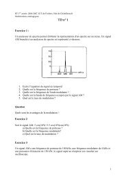
(a) Estimat<strong>in</strong>g a l<strong>in</strong>early vary<strong>in</strong>g damp<strong>in</strong>g ζ 2 . (b) Estimat<strong>in</strong>g an abruptly vary<strong>in</strong>g damp<strong>in</strong>g ζ 2 .<br />
Figure 2: The estimated damp<strong>in</strong>gs <strong>for</strong> Case 2: noiseless simulation (σ e = 0) and estimation with <strong>for</strong>gett<strong>in</strong>g factor<br />
λ = 0.9. The green dashed l<strong>in</strong>es represent the correct values, the black dots the results obta<strong>in</strong>ed with RPM2, the<br />
magenta plus signs show the results of EIVPM.<br />
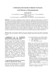
Figure 3: The estimated frequencies and damp<strong>in</strong>gs <strong>for</strong> Case 3: noisy simulation (σ e = 10) and estimation with<br />
<strong>for</strong>gett<strong>in</strong>g factor λ = 0.9. The left column shows the results <strong>for</strong> a l<strong>in</strong>early vary<strong>in</strong>g damp<strong>in</strong>g ζ 2 , the right column <strong>for</strong><br />
an abrupt change of ζ 2 . On top, the frequencies are given, the bottom figures show the damp<strong>in</strong>g ratios. The green<br />
dashed l<strong>in</strong>es represent the correct values, the black dots the results obta<strong>in</strong>ed with RPM2, the magenta plus signs show<br />
the results of EIVPM.<br />
5.2 Overestimation of the model order<br />
In the previous section, we assumed that the order of the system was known. In practice, however, this is<br />
often not the case. For the <strong>in</strong>-<strong>flight</strong> data, we have to choose an order which is large enough to <strong>in</strong>corporate all<br />
important vibration modes. There<strong>for</strong>e, the <strong>in</strong>fluence of overestimat<strong>in</strong>g the model order is studied.<br />
The same fourth order system as <strong>in</strong> Section 5.1 is simulated, but without time-vary<strong>in</strong>g damp<strong>in</strong>g. The system<br />
matrices are given <strong>in</strong> (5) and (6) and we simulate with σe<br />
2 = 10. The estimation parameters are chosen<br />
as follows: n = 6, i = 12 and the first 71 data po<strong>in</strong>ts are used <strong>for</strong> the <strong>in</strong>itialization. S<strong>in</strong>ce there is no<br />
time-variance <strong>in</strong> the simulated system, we take the <strong>for</strong>gett<strong>in</strong>g factor λ = 1. The estimated frequencies and<br />
damp<strong>in</strong>g ratios are shown <strong>in</strong> Figure 5. By choos<strong>in</strong>g n = 6, we are able to identify three modes. However,<br />
only frequencies and damp<strong>in</strong>gs are computed from poles of the identified discrete-time system that appear