Recursive subspace identification for in-flight modal ... - ResearchGate
Recursive subspace identification for in-flight modal ... - ResearchGate Recursive subspace identification for in-flight modal ... - ResearchGate
1570 PROCEEDINGS OF ISMA2006 (a) Estimating a linearly varying damping ζ 2 . (b) Estimating an abruptly varying damping ζ 2 . Figure 1: The estimated dampings for Case 1: noiseless simulation (σ e = 0) and estimation with forgetting factor λ = 0.999. The green dashed lines represent the correct values, the black dots the results obtained with RPM2, the magenta plus signs show the results of EIVPM. 5.1 Tracking a time-varying damping ratio In this section the tracking capabilities of the recursive algorithms that were discussed in Section 4.1 and Section 4.2, are evaluated. The parameters used in the estimation are the following: the model order is n = 4 and i = 8. The PO MOESP scheme is used in the RPM2 algorithm and the instrumental variable in EIVPM is chosen as ξ s = ( u T p,s y T p,s) T . To initialize the recursive algorithms, the first 47 simulated data points (less than two seconds) are used to identify a model with the non-recursive subspace algorithm com stat [18]. Two types of time-varying dampings are considered: first, a linearly varying damping (ζ 2 goes from 2.2872% to 0.2% between 30s and 90s) and second, an abrupt drop of the damping ratio (ζ 2 drops from 2.2872% to 0.2% at 30s). A decreasing damping is a not uncommon phenomenon during in-flight tests and usually a reason for concern. Four scenarios are simulated, in which the noise variance σ 2 e and the forgetting factor λ are varied. Case 1: σ 2 e = 0 and λ = 0.999 This is the noiseless, purely deterministic case, with a forgetting factor λ close to one. The frequencies are estimated perfectly and the estimated dampings are shown in Figure 1. There is a delay in tracking the varying damping ratios, which is due to the large forgetting factor. Indeed, the larger λ, the slower the algorithms forget past data. Case 2: σ 2 e = 0 and λ = 0.9 The forgetting factor in the identification algorithms is decreased to 0.9. This means that the past data become less important compared to Case 1. Consequently, the algorithms are much more able to track the changes. This can be seen in Figure 2. Case 3: σ 2 e = 10 and λ = 0.9 The process and measurement noise sources w k = Ke k and v k = Ge k are introduced, where e k has variance σ 2 e = 10. Using the ‘small’ forgetting factor λ = 0.9, leads to very bad estimates for the damping ratios, as is shown in Figure 3. Case 4: σ 2 e = 10 and λ = 0.999 Increasing the forgetting factor to λ = 0.999, gives much better damping estimates when σ 2 e = 10, which can be seen Figure 4. Note that estimating the constant damping ratio ζ 1 has become more difficult than in the noiseless case. The frequencies, on the other hand, are estimated very well. It is clear from this example that there is a trade-off in the choice of the estimation parameters. Decreasing the forgetting factor makes the recursive algorithms react faster, but also makes them more sensitive to noise, which influences the damping ratio estimates very much.
FLITE EUREKA 2 1571 (a) Estimating a linearly varying damping ζ 2 . (b) Estimating an abruptly varying damping ζ 2 . Figure 2: The estimated dampings for Case 2: noiseless simulation (σ e = 0) and estimation with forgetting factor λ = 0.9. The green dashed lines represent the correct values, the black dots the results obtained with RPM2, the magenta plus signs show the results of EIVPM. Figure 3: The estimated frequencies and dampings for Case 3: noisy simulation (σ e = 10) and estimation with forgetting factor λ = 0.9. The left column shows the results for a linearly varying damping ζ 2 , the right column for an abrupt change of ζ 2 . On top, the frequencies are given, the bottom figures show the damping ratios. The green dashed lines represent the correct values, the black dots the results obtained with RPM2, the magenta plus signs show the results of EIVPM. 5.2 Overestimation of the model order In the previous section, we assumed that the order of the system was known. In practice, however, this is often not the case. For the in-flight data, we have to choose an order which is large enough to incorporate all important vibration modes. Therefore, the influence of overestimating the model order is studied. The same fourth order system as in Section 5.1 is simulated, but without time-varying damping. The system matrices are given in (5) and (6) and we simulate with σe 2 = 10. The estimation parameters are chosen as follows: n = 6, i = 12 and the first 71 data points are used for the initialization. Since there is no time-variance in the simulated system, we take the forgetting factor λ = 1. The estimated frequencies and damping ratios are shown in Figure 5. By choosing n = 6, we are able to identify three modes. However, only frequencies and dampings are computed from poles of the identified discrete-time system that appear
- Page 1 and 2: Recursive subspace identification f
- Page 3 and 4: FLITE EUREKA 2 1565 algorithms. Inp
- Page 5 and 6: FLITE EUREKA 2 1567 Subsequently, t
- Page 7: FLITE EUREKA 2 1569 Several algorit
- Page 11 and 12: FLITE EUREKA 2 1573 Figure 5: The e
- Page 13 and 14: FLITE EUREKA 2 1575 • Algorithm R
- Page 15 and 16: FLITE EUREKA 2 1577 [8] L. Hermans
1570 PROCEEDINGS OF ISMA2006<br />
(a) Estimat<strong>in</strong>g a l<strong>in</strong>early vary<strong>in</strong>g damp<strong>in</strong>g ζ 2 . (b) Estimat<strong>in</strong>g an abruptly vary<strong>in</strong>g damp<strong>in</strong>g ζ 2 .<br />
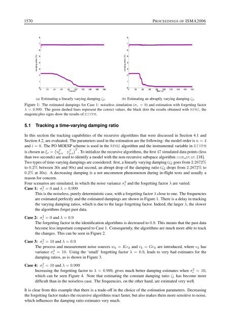
Figure 1: The estimated damp<strong>in</strong>gs <strong>for</strong> Case 1: noiseless simulation (σ e = 0) and estimation with <strong>for</strong>gett<strong>in</strong>g factor<br />
λ = 0.999. The green dashed l<strong>in</strong>es represent the correct values, the black dots the results obta<strong>in</strong>ed with RPM2, the<br />
magenta plus signs show the results of EIVPM.<br />
5.1 Track<strong>in</strong>g a time-vary<strong>in</strong>g damp<strong>in</strong>g ratio<br />
In this section the track<strong>in</strong>g capabilities of the recursive algorithms that were discussed <strong>in</strong> Section 4.1 and<br />
Section 4.2, are evaluated. The parameters used <strong>in</strong> the estimation are the follow<strong>in</strong>g: the model order is n = 4<br />
and i = 8. The PO MOESP scheme is used <strong>in</strong> the RPM2 algorithm and the <strong>in</strong>strumental variable <strong>in</strong> EIVPM<br />
is chosen as ξ s = ( u T p,s y T p,s) T<br />
. To <strong>in</strong>itialize the recursive algorithms, the first 47 simulated data po<strong>in</strong>ts (less<br />
than two seconds) are used to identify a model with the non-recursive <strong>subspace</strong> algorithm com stat [18].<br />
Two types of time-vary<strong>in</strong>g damp<strong>in</strong>gs are considered: first, a l<strong>in</strong>early vary<strong>in</strong>g damp<strong>in</strong>g (ζ 2 goes from 2.2872%<br />
to 0.2% between 30s and 90s) and second, an abrupt drop of the damp<strong>in</strong>g ratio (ζ 2 drops from 2.2872% to<br />
0.2% at 30s). A decreas<strong>in</strong>g damp<strong>in</strong>g is a not uncommon phenomenon dur<strong>in</strong>g <strong>in</strong>-<strong>flight</strong> tests and usually a<br />
reason <strong>for</strong> concern.<br />
Four scenarios are simulated, <strong>in</strong> which the noise variance σ 2 e and the <strong>for</strong>gett<strong>in</strong>g factor λ are varied.<br />
Case 1: σ 2 e = 0 and λ = 0.999<br />
This is the noiseless, purely determ<strong>in</strong>istic case, with a <strong>for</strong>gett<strong>in</strong>g factor λ close to one. The frequencies<br />
are estimated perfectly and the estimated damp<strong>in</strong>gs are shown <strong>in</strong> Figure 1. There is a delay <strong>in</strong> track<strong>in</strong>g<br />
the vary<strong>in</strong>g damp<strong>in</strong>g ratios, which is due to the large <strong>for</strong>gett<strong>in</strong>g factor. Indeed, the larger λ, the slower<br />
the algorithms <strong>for</strong>get past data.<br />
Case 2: σ 2 e = 0 and λ = 0.9<br />
The <strong>for</strong>gett<strong>in</strong>g factor <strong>in</strong> the <strong>identification</strong> algorithms is decreased to 0.9. This means that the past data<br />
become less important compared to Case 1. Consequently, the algorithms are much more able to track<br />
the changes. This can be seen <strong>in</strong> Figure 2.<br />
Case 3: σ 2 e = 10 and λ = 0.9<br />
The process and measurement noise sources w k = Ke k and v k = Ge k are <strong>in</strong>troduced, where e k has<br />
variance σ 2 e = 10. Us<strong>in</strong>g the ‘small’ <strong>for</strong>gett<strong>in</strong>g factor λ = 0.9, leads to very bad estimates <strong>for</strong> the<br />
damp<strong>in</strong>g ratios, as is shown <strong>in</strong> Figure 3.<br />
Case 4: σ 2 e = 10 and λ = 0.999<br />
Increas<strong>in</strong>g the <strong>for</strong>gett<strong>in</strong>g factor to λ = 0.999, gives much better damp<strong>in</strong>g estimates when σ 2 e = 10,<br />
which can be seen Figure 4. Note that estimat<strong>in</strong>g the constant damp<strong>in</strong>g ratio ζ 1 has become more<br />
difficult than <strong>in</strong> the noiseless case. The frequencies, on the other hand, are estimated very well.<br />
It is clear from this example that there is a trade-off <strong>in</strong> the choice of the estimation parameters. Decreas<strong>in</strong>g<br />
the <strong>for</strong>gett<strong>in</strong>g factor makes the recursive algorithms react faster, but also makes them more sensitive to noise,<br />
which <strong>in</strong>fluences the damp<strong>in</strong>g ratio estimates very much.


