Comparison of two worst-case response time analysis ... - LIAS

Comparison of two worst-case response time analysis methods for
real-time transactions
A. Rahni, K. Traore, E. Grolleau and M. Richard
LISI/ENSMA
Téléport 2, 1 Av. Clément Ader
BP 40109, 86961 Futuroscope Chasseneuil Cedex
{rahnia,traore,grolleau,richardm}@ensma.fr
Abstract
This paper presents a comparison of two worst
case response time analysis methods in the context of
transactions. In the general context of tasks with offsets
(general transactions), only exponential methods
are known to calculate the exact worst-case response
time of a task. We focus more precisely on monotonic
transactions. In this context, we present the fast
and tight analysis, proposed in [7, 6], and the analysis
technique of monotonic transaction that we have
proposed in [14]. We compare them on a case study
and on several configurations generated randomly.
Keywords: Response Time, Transactions
1. Introduction
The Response-Time Analysis [1] is an essential
analysis technique that can be used to perform
schedulability tests. Tindell proposed in [11] a new
model of tasks with offset (transactions) extending
the model of Liu and Layland [5]. Since the transactions
are non-concrete(the transaction release times
are not fixed a priori), the main problems is to determine
the worst case configuration for a task under
analysis (its critical instant). Tindell showed that the
critical instant for a task under analysis (τ ua ) occurs
when one task of higher priority in each transaction
is released at the same time as τ ua .
An exact calculation method has been proposed
in [10], but has an exponential complexity and is
intractable for realistic task systems; Tindell [11]
has proposed a pseudo-polynomial approximation
method providing an upper bound of the worst-case
response-time. Later, this approach has been improved
in [4, 6, 7, 8]
In the sequel, we present the model of tasks with
offsets (a.k.a. transaction), then we present the best
known approximation method proposed by Turja and
Nolin [8]. Section 4 presents the monotonic transactions
exact analysis [13] and these two methods are
used on the same tasks system. In the last section
their performance are compared on randomly generated
transaction systems.
2. Model of transactions
A tasks system Γ is composed of a set of |Γ| transactions
Γ i , with 1 ≤ i ≤ |Γ i | (where |Γ i | is the number
of elements in the set Γ i ).
{ }
Γ : Γ1 , Γ 2 , .., Γ |Γ|
{ }
Γ i : τi1 , τ i2 , ..., τ i|Γi|, T i
τ ij : < C ij , O ij , D ij , J ij , B ij , P ij >
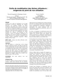
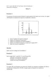
Each transaction Γ i (see figure 1) consists of a set
of |Γ i | tasks τ ij released at the same period T i , with
0 < j ≤ |Γ|. Without loss of generality, we suppose
that the tasks are ordered in the set by increasing
offset. A task τ ij is defined by : a worst-case execution
time (WCET) C ij , an offset O ij related to the
release date of the transaction Γ i , a relative deadline
D ij , a maximum jitter J ij (the activation time
of task τ ij may occur at any time between t 0 + O ij
and t 0 + O ij + J ij , where t 0 is the release date of the
transaction Γ i , a maximum blocking factor B ij due
to lower priority tasks (e.g. priority ceiling protocol
[9]), and P ij is its priority (we assume a fixed-priority
scheduling policy). The figure 1 presents an example
of transaction Γ i composed of three tasks with period
T i = 16.
Let us note hp i (τ ua ) the set of indices of the tasks of
Γ i with a priority higher than the priority of a task
under analysis τ ua , assuming that the priorities of the
tasks are unique.
3 Fast and Tight Analysis
This method provides an efficient implementation
to calculate an upper-bound of the worst-case response
times [7]. The main idea is to represent the
periodic interference function statically, and during

f
r
f
g
τ τ
W%(τ&',t )
Figure 1. Example of transaction.
Γ
Γ ¡¢£¤ ©¡¦ ©¡
O§ © ¡
τ ¡
the response-time calculation, to use a simple lookup
function in order to compute its value. The interference
imposed by the transaction Γ i on a task under
analysis τ ua during a busy period of length t starting
at the release of τ ua and corresponding to the release
of τ ic is noted W ic (τ ua , t) (τ ic is then called the critical
instant candidate in Γ i ). In order to simplify, we
suppose no Jitter in the transaction (i.e J ij = 0).
¥¡¦O§¨
W ic (τ ua, t) =
τ
τ τ
τ τ
∑
j∈hp i (τ ua)
t ∗ = t − Φ ijc
((⌊ t ∗ ⌋ )
)
+ 1 ∗ C ij − x ijc (t)
T i
Φ ijc = (T i + (O ij − O ic )) % T i
{ 0 for t
x ijc (t) =
∗ < 0
max(0, C ij − (t ∗ % T i )) otherwise
Φ ijc is the phase between τ ic and τ ij . x ijc (t) corresponds
to the part of the task τ ij that cannot be
executed in the time interval of length t (note that
this part is the main difference between the methods
presented in [4] and [7]).
In order to find the critical instant, one would have to
compare every combination of critical instant candidates,
making the exact test intractable. The fast and
tight analysis method consists of creating a global interference
function W i (τ ua , t) for each transaction Γ i ,
in choosing the maximum value of each interference
function.
W i (τ ua , t) =
max W ic(τ ua , t)
∀c∈hp i(τ ua)
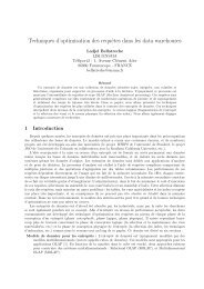
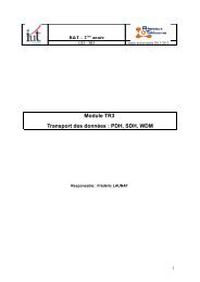
The figure 2 shows the graphical representation of
the interference of a transaction : each curve represents
the interference function for each critical instant
candidate. Since the transaction is in normal form,
the derivative of each curve is either 0 or 1. W i (τ ua , t)
that has to be computed is the maximum of all the
curves. The efficient implementation proposed in [7]
stores the set of points P ic , where each point P ic [k]
has an x (representing time) and a y (representing
interference) coordinate. These points correspond to
the convex corners of the curve W ic (τ ua , t).
The calculation of the upper bound on the worst-case
response time R ua of τ ua is obtained by an iterative
Figure 2. Interference of transaction.
!" τ
#$ #
fix-point lookup.
R 0 ua = C ua
R (n+1)
ua
= C ua + ∑ Γ i∈Γ
(W i (τ ua , R n ua )) (1)
where W i (τ ua , t) is deduced from the static representation
of the transactions interferences.
3.1 Normal form of a transaction
Without loss of generality, we consider that all the
tasks of Γ i have a higher priority than the task under
analysis τ ua . Since some tasks of a transaction may
have to overlap, issuing in an interference function
which derivative would be greater than 1, a normal
form of the transaction is first obtained using three
operations: order, merge, and split [7]. For each critical
instant candidate τ ic , the transaction Γ i is put in
normal-form. We start with all the tasks numbered
in increasing Φ ijc (phase between τ ij and τ ic ). Thus
the task τ ic in the original transaction is named τ i1
at the beginning of the normal-form processing.
The underlying idea behind the merge operation is
that if two tasks τ ij and τ ij+1 overlap, then the
longest busy period initiated by τ ij is always including
the longest busy period initiated by τ ij+1 . The
split operation is used when a part of a task has to be
executed during the next period of the transaction :
in this case the spilling task is splitted into two tasks.
The spilling part is taken into account as a task with
an offset equal to 0 in the second period of the transaction.
Thus, since the tasks are numbered according
to the increasing value of Φ ijc , the tasks can be renumbered
(ordering operation) in the second period
of the transaction. These operations are used until
no task in the transaction is forced to overlap on the
next one, and until no task is forced to spill in the
second period of the transaction.
Note that the first period of a transaction may differ
in the number of tasks from the second period due to
the spilling tasks.
Note that if a jitter has to be taken into account, this
operation has to be done for every critical instant
2

candidate.
3.2 Example
We apply this method on the transaction Γ i that
contains twelve tasks with no jitter (J ij = 0). and the
task τ ua with a WCET C ua = 9 and a lower priority
than all the tasks of Γ i .
Γ i := {< τ i1τ i2, ..., τ i12 >,60}
τ i1 :< 3, 1, D i1, 0,0, 1 > τ i7 :< 2, 36, D i7,0, 0,7 >
τ i2 :< 4, 9, D i2, 0,0, 2 > τ i8 :< 5, 43, D i8,0, 0,8 >
τ i3 :< 2,11, D i3, 0,0, 3 > τ i9 :< 3, 46, D i9,0, 0,9 >
τ i4 :< 3,20, D i4, 0,0, 4 > τ i10 :< 1,49, D i10,0, 0,10 >
τ i5 :< 4,29, D i5, 0,0, 5 > τ i11 :< 4,56, D i11,0, 0,11 >
τ i6 :< 5,31, D i6, 0,0, 6 > τ i12 :< 2,57, D i12,0, 0,12 >
Obtaining the normal-form for Γ i for the critical
instant candidate τ i1 : the three operations (order,
merge and spill), merge τ i3 in τ i2 , τ i6 and τ i7 in τ i5 ,
τ i9 and τ i10 are merged in τ i8 , and τ i11 is merged in
τ i12 . The last task spills in the next period, thus the
second period of the transaction (and the following)
will have a additional task The resulting transaction
in normal-form, for the first period is:
τ i1 :< 3,0, D i1,0,0, 1 > τ i2 :< 6,8, D i2,0, 0,2 >
τ i3 :< 3, 19, D i3,0,0, 3 > τ i4 :< 11, 28, D i4,0,0, 4 >
τ i5 :< 9, 42, D i5,0,0, 5 > τ i6 :< 5,55, D i6,0, 0, 6 >
For the second period, the spilling time of the original
τ i12 is taken into account in the first task τ i1 of the
second period of the transaction, obtaining a WCET
of 4.
τ i1 :=< 4, 0, D i1,0, 0,1 > τ i2 :=< 6,8, D i2,0, 0,2 >
τ i3 :=< 3,19, D i3,0, 0,3 > τ i4 :=< 11, 28, D i4,0, 0,4 >
τ i5 :=< 9,42, D i5,0, 0,5 > τ i6 :=< 5,55, D i6,0,0, 6 >
The same operation is done for all the task
candidates τ ic for c = 2..12. The upper bound of
the worst-case response time is then obtained using
formula 1:
Iteration 0 : R 0 ua = 9
Iteration 1 : t = 9 : R 1 ua = 9 + 11 = 20
Iteration 2 : t = 20 : R 2 ua = 9 + 20 = 29
Iteration 3 : t = 29 : R 3 ua = 9 + 29 = 38
Iteration 4 : t = 38 : R 4 ua = 9 + 29 = 38
4 Monotonic Transactions
In this section we present the different steps of
monotonic transaction analysis [13, 14, 12]. Monotonic
transaction analysis relies on transactions for
which one interference curve (for one candidate) is
always greater or equal than the other curves. In
this way, it’s close to the concept of accumulatively
monotonic generalized multiframe task sets [2]. In
this case, if a transaction Γ i is monotonic then the
critical instant occurs when the task under analysis
is released at the same time as the first task of the
pattern of the normal form of Γ i . Therefore, for the
case where all the transactions of the task system are
monotonic for a task under analysis, the computed
worst-case response time is exact.
Since there is only one possible candidate in a
monotonic transaction, there is only one normal-form
to compute.
4.1 Finding the monotonic pattern
Let Γ ∗ i be
{
the normal form of
}
the transaction Γ i
where Γ ∗ i :< τi1 ∗ , τ i2 ∗ , ..., τ i|Γ ∗ ∗|, T i , T i > and Γ i :<
{ }
i
τi1 , τ i2 , ..., τ i|Γi|, T i , Ti >. Let us note:
α ij = O ∗ i(j+1) − (O∗ ij + C ∗ ij) for 1 ≤ j < |Γ ∗ i |
α i|Γ ∗
i | = (T i + O ∗ i1 ) − (O∗ i|Γ ∗ i | + C∗ i|Γ ∗ i |)
where α ij > 1 since Γ ∗ i is in normal form.
Note that since it’s not necessary to statically store
the interference function, there is no need to make a
difference between the first and the second period of
the transaction.
Γ i is a monotonic transaction for the task τ ua (we
consider that all the tasks of Γ i have a higher priority
than the one of τ ua ) if the WCET of the tasks of Γ ∗ i
have decreasing values while the idle slots α ij have
increasing values i.e: Ci(p+1) ∗ ≤ C∗ ip for all 1 ≤ p <
|Γ ∗ i | and α ip ≤ α i(p+1) for all 1 ≤ p < |Γ ∗ i |.
Γ i is monotonic if we can find a monotonic pattern
in Γ ∗ i by rotating the tasks of Γ∗ i . We know that for
a monotonic pattern the first task has the highest
WCET. In order to look for a monotonic pattern, we
start by inventorying all the tasks with the maximum
WCET. Then, we consider alternatively each of these
tasks τik ∗ as the first task of the transaction Γ∗ i by rotating
the tasks of Γ ∗ i ; and we verify if the conditions
of monotony (on Cij ∗ and α ij) are respected; if so, Γ i
is monotonic and τik ∗ become the first task of Γ∗ i .
4.2 Example
We apply this method on the same example as the
one we used for the fast and tight analysis.
We find Γ ∗ i the normal form of the transaction Γ i by
applying the operations of normalization process:
Γ ∗ i : {< τ ∗ i1, τ ∗ i2, ..., τ ∗ i5 >,60}
τ ∗ i1 :< 6, 9, D i1,0,0, 1 > τ ∗ i2 :< 3,20, D i2,0, 0,2 >
τ ∗ i3 :< 11,29, D i3,0,0, 3 > τ ∗ i4 :< 9,43, D i4,0, 0,4 >
τ ∗ i5 :< 9,56, D i5,0,0, 5 >
3

We have: α ∗ i1 = 5, α∗ i2 = 6, α∗ i3 = 3, α∗ i4 = 4, α∗ i5 = 4
There is a monotonic pattern starting from task τ ∗ i3
where:
C ∗ i3 ≥ C ∗ i4 ≥ C ∗ i5 ≥ C ∗ i1 ≥ C ∗ i2
α ∗ i3 ≤ α ∗ i4 ≤ α ∗ i5 ≤ α ∗ i1 ≤ α ∗ i2
Hence the transaction is monotonic, and the critical
instant of τ ua corresponds to the release of the task
τi3 ∗ , we apply the iterative fix-point lookup in order
to calculate the worst-case response time of τ ua .
In the case of monotonic transactions, the two methods
presented provide the same exact worst-case response
time with the same number of iterations in
the process of calculation, because in every iteration,
the task that initiates the critical instant is the same.
The only difference between these two methods comes
from the stage of static representation in the fast and
tight analysis (stage A) and the research of the monotonic
pattern for the method of monotonic transaction
(stage B). Stage A for n tasks requires at least
n normal-form processing, plus computing the static
tables. Stage B requires only one normal-form processing
operation and a linear complexity test in order
to check the conditions related to Ci ∗ and α ∗ i .
5. Performance comparison and future
works
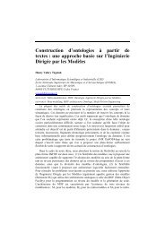
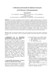
We have implemented the two methods in order to
compare their respective performance. The figure 3
shows that the time used by the method proposed in
[8]increases linearly with the number of transactions,
while the method proposed in [14] is less sensitive to
the size of the system when only monotonic transactions
are involved. The tests have been led on a Pentium
IV processor, for sets of 20 configurations per
number of transactions. The transactions are monotonic,
and contain 15 tasks, while the workload is
fixed around 0.8. The random generation system is
based on the UUniFast algorithm presented in [3].
The bound on the worst-case response time is the
same for both methods, since at this stage, montonicity
is more a characterization allowing an optimization
than a method by itself (it has still to be coupled
with the method of [8] because in a system of transactions,
the transactions don’t have to be all monotonic).
In future works, we will use the monotonicity property
as a basement to introduce a new evaluation
method in order to decrease the pessimism of [8] for
the upper bound on the worst-case response times.
References
[1] N. Audsley, A. Burns, R. Davis, K. Tindell, and
A. Wellings. Fixed priority pre-emptive scheduling:
An historical perspective. Real-Time Systems
8, pages 129–154, 1995.
Execution times
140
120
100
80
60
40
20
0
1
4
7
10
13
16
19
22
25
28
31
34
37
Number of transactions of 15 tasks
Figure 3. Execution time
Fast-Tight
Monotonic
[2] S. Baruah, D. Chen, S. Gorinsky, and A. Mok. Generalized
multiframe tasks. The International Journal
of Time-Critical Computing Systems, (17):5–22,
1999.
[3] E. Bini and G. Buttazzo. Biasing effects in
schedulablity measures. IEEE Proceedings of the
16th Euromicro Conference on Real-Time Systems
(ECRTS04), Catania, Italy, (16), July 2004.
[4] J. P. Gutierrez and M. G. Harbour. Schedulability
analysis for tasks with static and dynamic offsets.
Proc IEEE Real-time System Symposium (RTSS),
(19), December 1998.
[5] C. Liu and J. Layland. Scheduling algorithms
for multiprogramming in real-time environnement.
Journal of ACM, 1(20):46–61, October 1973.
[6] J. Maki-Turja and M. Nolin. Faster response time
analysis of tasks with offsets. Proc 10th IEEE
Real-Time Technology and Applications Symposium
(RTAS), May 2004.
[7] J. Maki-Turja and M. Nolin. Tighter response time
analysis of tasks with offsets. Proc 10th International
Conference on Real-Time Computing and Applications
(RTCSA04, August 2004.
[8] J. Maki-Turja and M. Nolin. Fast and tight responsetimes
for tasks with offsets. 17th EUROMICRO Conference
on Real-Time Systems IEEE Palma de Mallorca
Spain, July 2005.
[9] L. Sha, R. Rajkumar, and J. Lehoczky. Priority
inheritance protocols : an approach to real-time
synchronization. IEEE Transactions on Computers,
39(9):1175–1185, 1990.
[10] K. Tindell. Using offset information to analyse static
priority pre-emptively scheduled task sets. Technical
Report YCD-182,Dept of Computer Science, Unoversity
of York, England, 1992.
[11] K. Tindell. Adding time-offsets to schedulability
analysis. Technical Report YCS 221, Dept of Computer
Science, University of York, England, January
1994.
[12] K. Traore. Analyse et Validation des Applications
Temps Réel en Présence de Transactions : Application
au Pilotage d’un Drone Miniature. Thèse,
ENSMA-Université Poitiers, 2007.
[13] K. Traore, E. Grolleau, and F. Cottet. Characterization
and analysis of tasks with offsets: Monotonic
transactions. Proc 12th International Conference on
Embedded and Real-Time Computing Systems and
4

Applications. RTCSA’06, (12), August 16-18th Sydney,
Australia 2006.
[14] K. Traore, E. Grolleau, A. Rahni, and M. Richard.
Response-time analysis of tasks with offsets. 12th
IEEE International Conference on Emerging Technologies
and Factory Automation ETFA’06, September
2006.
5