Design of an Active 1-DOF Lower-Limb Exoskeleton with ... - Colgate

Design of an Active 1-DOF Lower-Limb Exoskeleton with Inertia
Compensation
Gabriel Aguirre-Ollinger, J. Edward Colgate, Michael A. Peshkin and Ambarish Goswami
September 2, 2010
Abstract
Limited research has been done on exoskeletons to enable faster movements of the lower extremities.
An exoskeleton’s mechanism can actually hinder agility by adding weight, inertia and friction to the legs;
compensating inertia through control is particularly difficult due to instability issues. The added inertia
will reduce the natural frequency of the legs, probably leading to lower step frequency during walking.
We present a control method that produces an approximate compensation of an exoskeleton’s inertia.
The aim is making the natural frequency of the exoskeleton-assisted leg larger than that of the unaided
leg. The method uses admittance control to compensate the weight and friction of the exoskeleton.
Inertia compensation is emulated by adding a feedback loop consisting of low-pass filtered acceleration
multiplied by a negative gain. This gain simulates negative inertia in the low-frequency range. We tested
the controller on a statically supported, single-DOF exoskeleton that assists swing movements of the leg.
Subjects performed movement sequences, first unassisted and then using the exoskeleton, in the context
of a computer-based task resembling a race. With zero inertia compensation, the steady-state frequency
of leg swing was consistently reduced. Adding inertia compensation enabled subjects to recover their
normal frequency of swing.
Keywords: Exoskeleton, rehabilitation robotics, lower-limb assistance, admittance control
1 Nomenclature
1.1 Symbols
I h , b h , k h = Moment of inertia (kg-m 2 ), damping (N-m-s/rad) and stiffness (N-m/rad) of the human
limb.
Īe d,¯b d e , ¯k e d = Virtual moment of inertia, damping and stiffness of the exoskeleton’s drive mechanism in
the controller’s admittance model.
I m = Moment of inertia of the exoskeleton’s servo motor, reflected on the output shaft.
b c , k c = Exoskeleton cable drive’s damping and stiffness.
I s = Exoskeleton’s output drive inertia (moment of inertia of the mechanical components between the
cable and the torque sensor).
I arm , b arm , k arm = Moment of inertia, damping and stiffness of the exoskeleton’s arm.
I c = Emulated inertia compensator’s gain (kg-m 2 ).
ω lo = Cutoff frequency (rad/s) of the inertia compensator’s low-pass filter.
ω n,e = Natural frequency of the exoskeleton drive.
τ h = Net muscle torque (N-m) acting on the human limb’s joint.
τ m = Torque exerted by the exoskeleton’s actuator.
1

τ s = Torque measured by the exoskeleton’s torque sensor.
w m = Angular velocity (rad/s) of the servo motor reflected on the output shaft.
w s = Angular velocity of the exoskeleton’s drive output shaft.
Ω h = RMS angular velocity (rad/s) of swing of the human limb.
f c = Frequency of leg swing (Hz).
A c = Amplitude of leg swing (rad).
x ref = Horizontal position (dimensionless) of the target cursor on the graphic user interface.
x h = Horizontal position of the subject’s cursor on the graphic user interface.
1.2 Transfer functions
Y e (s) = Two-port admittance of the physical exoskeleton’s drive.
Ȳe d (s) = Virtual admittance model followed by the admittance controller. It represents the desired
admittance of the torque sensor port.
Y s
e (s) = Actual closed-loop admittance at the torque sensor port.
Y p
e (s) = Closed-loop admittance at the exoskeleton’s port of interaction with the user (ankle brace).
Y h
e (s) = Admittance of the human leg when coupled to the exoskeleton (defined as the ratio of w s (s)
to τ h (s)).
Z arm (s) = Impedance of the exoskeleton’s arm.
Z h (s) = Impedance of the human limb.
2 Introduction
In recent years, different types of exoskeletons and orthotic devices have been developed to assist lower-limb
motion. Applications for these devices usually fall into either of two broad categories: (1) augmenting the
muscular force of healthy subjects, and (2) rehabilitation of people with motion impairments. Most of the existing
implementations in the former group are designed to either enhance the user’s capability to carry heavy
loads [Lee and Sankai, 2003, Kawamoto and Sankai, 2005, Kazerooni et al., 2005, Walsh et al., 2006] or reduce
muscle activation during walking [Banala et al., 2006, Sawicki and Ferris, 2009, Lee and Sankai, 2002].
Rehabilitation-oriented applications include training devices for gait correction [Jezernik et al., 2004, Banala et al., 2009]
and devices that apply controlled forces to the extremities in substitution of a therapist [Veneman et al., 2007].
Although significant advances have been made in the engineering aspects of exoskeleton design (mechatronics,
computer control, actuators), the physiological aspects of wearing an exoskeleton are less well understood.
A common observation in recent reviews on exoskeleton research [Ferris et al., 2005, Ferris et al., 2007,
Dollar and Herr, 2008] has been the absence of reports of exoskeletons reducing the metabolic cost of walking.
Another little-researched topic has been the effect of an exoskeleton on the agility of the user’s movements.
At this point we are not aware of any studies addressing how an exoskeleton can affect the user’s selected
speed of walking, or the ability to accelerate the legs when quick movements are needed.
The present study constitutes a first step towards enabling an exoskeleton to increase the agility of the
lower extremities. At preferred walking speeds, the swing leg behaves as a pendulum oscillating close to
its natural frequency [Kuo, 2001]. The swing phase of walking takes advantage of this pendular motion in
order to reduce the metabolic cost of walking. Thus we theorize that a wearable exoskeleton could be used
to increase the natural frequency of the legs, and in doing so enable users to walk comfortably at higher
speeds. Although a few studies have been conducted on the modulation of leg swing frequency by means of
2

an exoskeleton [Uemura et al., 2006, Lee and Sankai, 2005], to the best of our knowledge this effect has not
yet been linked experimentally to the kinematics and energetics of walking.
The main difficulty in using an exoskeleton to increase the agility of leg movements is that the exoskeleton’s
mechanism adds extra impedance to the legs. Therefore the mechanism by itself can be expected to
make the legs’ movements slower, not faster. And while it is quite feasible to mask the weight and the
friction of the mechanism using control, compensating the mechanism’s inertia is considerably more difficult
due to stability issues [Newman, 1992, Buerger and Hogan, 2007]. All other things being equal, the inertia
added by the exoskeleton will probably reduce the pendulum frequency of the legs, which can have important
consequences on the metabolic cost and the speed of walking. A study by Browning [Browning et al., 2007]
found that adding masses to the leg increases the metabolic cost of walking. This cost was strongly correlated
to the moment of inertia of the loaded leg. A similar study by Royer [Royer and Martin, 2005] showed
that loading the legs increases the swing time and the stride time during walking. The findings from both
studies may be explained by the metabolic cost of swinging the leg. In an experiment reported by Doke
[Doke et al., 2005], subjects swung one leg freely at different frequencies with fixed amplitude. It was found
that the metabolic cost of swinging the leg has a minimum near the natural frequency of the leg, and increases
with the fourth power of frequency. Thus if the exoskeleton’s inertia reduces the natural frequency
of the leg it is very likely that users will reduce their chosen frequency of leg swing accordingly.
The notion of compensating the inertia of the exoskeleton through control leads to an interesting prospect:
to not only compensate the drop in the natural frequency of the legs caused by the exoskeleton’s mechanism,
but to actually make the natural frequency of the exoskeleton-assisted leg higher than that of the unaided leg.
This in turn raises two possible research questions. First, if the exoskeleton modifies the natural frequency
of the leg, will people modify their frequency of leg swing accordingly? Second, how does the behavior of
metabolic cost change when the natural frequency is modified, i.e. does the new natural frequency accurately
predict the minimum metabolic cost?
In this paper we address the first question. We present a control method that produces an approximate
compensation of an exoskeleton’s inertia. We tested our method on a statically mounted, single-DOF exoskeleton
[Aguirre-Ollinger et al., 2007b, Aguirre-Ollinger et al., 2007a] that assists the user in performing
knee flexions and extensions. The exoskeleton has a “baseline” mode of operation in which an admittance
controller masks the the weight and the dissipative effects (friction, damping) of the exoskeleton’s mechanism,
thereby making the exoskeleton behave as a pure inertia. An acceleration feedback loop is then added
to compensate the exoskeleton’s inertia at low frequencies. We conducted an experiment in which subjects
performed multiple series of leg-swing movements in the context of a computer-based pursuit task. Subjects
moved their leg under three different experimental conditions: (1) leg unaided, (2) wearing the exoskeleton in
“baseline” state and (3) wearing the exoskeleton with inertia compensation on. The effects of the exoskeleton
on the frequency of leg swing are analyzed and discussed.
3 Exoskeleton design and construction
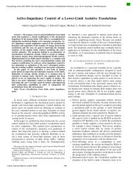
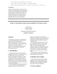
We designed and built a stationary 1-DOF exoskeleton for assisting knee flexion and extension exercises
(Figure 1). Our aim was to use the pendular motion of the leg’s shank as a scaled-down model of the swing
motion of the entire leg when walking, and to investigate the effects of an active exoskeleton dynamics on
the kinematics and energetics of leg-swing motion.
In order to specify the torque requirements for our 1-DOF exoskeleton, we surveyed reported values of
knee torque during normal walking. Kerrigan [Kerrigan et al., 2000] reported an extensive study on the knee
joint torques of barefoot walking. The peak knee torques reported there were 0.340.15 N-m/kg-m for women
and 0.320.15 N-m/kg-m for men. Thus for a male subject with body mass of 80 kg and height of 1.80 m, the
peak knee torque during normal walking should be about 45 N-m. DeVita [DeVita and Hortobagyi, 2003]
reported peak knee torques ranging from 0.39 N-m/kg for obese subjects to 0.97 N-m/kg for lean subjects.
From these data, we concluded that an actuator-transmission combination capable of delivering about 20
N-m of continuous torque would be sufficient to produce significantly large assistive torques.
Figure 2 shows a CAD model of the exoskeleton’s main assembly, consisting of a servo motor, a cable-drive
transmission and a pivoting arm. The motor is a Kollmorgen (Radford, VA, USA) brushless direct-drive AC
motor with a power rating of 0.99 kW and a continuous torque rating of 2.0 N-m. The motor features a
3

Figure 1: 1-DOF exoskeleton coupled to a subject’s leg.
proprietary emulated encoder with a resolution is 65,536 counts. The transmission ratio of the exoskeleton’s
cable drive is 10:1, thus allowing a continuous torque output of 20.0 N-m. The exoskeleton arm, fabricated
in aluminum, has been made as lightweight as possible in order to reduce its inertial effects. The angular
acceleration of the exoskeleton arm is measured by means of an MT9 digital inertial measurement unit from
Xsens Technologies (Enschede, the Netherlands), operating at a sampling rate of 200 Hz . The unit features
a 3-axis linear accelerometer, and is mounted in such a way that two of the axes lie on the plane of rotation
of the exoskeleton’s arm (Figure 3). Angular acceleration is computed from the readings generated by those
two axes.
The cable-drive solution was chosen in order to avoid problems associated with transmission backlash.
Implementing admittance control in a system with a geared transmission can give rise to limit cycles due
to backlash, particularly when damping compensation is applied [Aguirre-Ollinger et al., 2007b]. A detail
of the exoskeleton’s drive system is shown in Figure 4. The torque sensor is located downstream from the
cable drive, enabling the controller to mask any friction occurring on the cable and the motor. The tension
of the cable is adjusted by means of a pair of adjustable plugs mounted on the inside of the major pulley.
For actual use the exoskeleton assembly is mounted on a rigid support frame (Figure 1). A custom-built
ankle brace (Figure 3) couples the user’s leg to the exoskeleton arm. The ankle brace is mounted on a sliding
bracket in order to accommodate any possible radial displacement of the ankle relative to the device’s center
of rotation.
4

Figure 2: Diagram of the 1-DOF exoskeleton’s motor, drive and arm assembly.
4 Assist through admittance control
In this section we discuss our general concept of exoskeleton-based assistance using admittance control. Then
we examine the question of whether an admittance controller can be used to compensate the inertia of the
user’s limb. A very simplified model of an admittance controller shows that, even assuming the very favorable
case of rigid coupling between the user’s limb and the exoskeleton, the coupled system will become unstable
before any inertia compensation is accomplished. However, an approximate form of inertia compensation
can be achieved by adding low-pass filtered acceleration feedback to the admittance controller.
Figure 5 shows a simplified model of the coupled system formed by the exoskeleton and the user’s limb.
Ideally, the admittance controller makes the exoskeleton drive (Figure 4) behave according to a virtual
admittance model consisting of inertia moment Īd e , damping coefficient ¯b d e , and stiffness coefficient ¯k d e :
Ȳ d
e (s) =
s
Ī d e s2 + ¯b d e s + ¯k d e
It can be seen on Figure 5 that the port of interaction between the user and the exoskeleton, P, is different
from the torque sensor port S. In the physical exoskeleton, P corresponds to the ankle brace. Due to
the impedance of the exoskeleton arm, these two ports have different admittances. The impedance of the
exoskeleton’s arm is given by
(1)
5

Figure 3: Mounting of the inertial measurement unit on the exoskeleton’s arm.
Z arm (s) = I arms 2 + b arm s + k arm
(2)
s
The most basic use of the admittance controller is to mask the dynamics of the exoskeleton arm from the
user. For example, if we include gravitational effects in the term k arm , the weight of the exoskeleton’s arm
can be balanced by making ¯k e d = −k arm . Likewise we can cancel the damping felt by the user by making
¯bd e = −b arm .
One attractive feature of the admittance controller is that it can transition seamlessly from masking
the impedance of the exoskeleton to actually assisting the user. For example, negative damping can be
rendered at the interaction port in order to transfer energy to the user’s limb. We have previously reported
experiments [Aguirre-Ollinger et al., 2007b, Aguirre-Ollinger et al., 2007a] in which negative damping was
used to assist leg motion. Although negative damping made the isolated exoskeleton unstable, the subjects
did remarkably well at maintaining control of their legs’ movements when using the exoskeleton. Those
experiments relied in part on the passive damping of the human limb to insure the stability of the coupled
system.
Our goal here is to make the exoskeleton increase the natural frequency of the leg, which can in theory
be accomplished by compensating the inertia of the leg. A possible strategy would be to generate a negative
drive inertia Īd e , and use the inertia of the human limb I h to guarantee the stability of the coupled system.
However, as we will show, non-collocation of the exoskeleton’s actuator and the torque sensor will cause the
coupled system to become unstable even for positive values of Īd e, if these are too low in magnitude.
5 Inertia compensation and sensor non-collocation
The effects of the torque sensor’s non-collocation can be demonstrated with a simplified model of the exoskeleton’s
mechanism and the human limb, shown in Figure 6. The drive portion of the exoskeleton’s
model consists of the servo motor’s inertia I m (reflected on the output shaft) and an output inertia I s , which
comprises the mechanical components located between the cable and the torque sensor, i.e. the major pulley
6

Figure 4: Detail of the exoskeleton mechanism. The shaded rectangle contains the drive system components:
grooved pulley (connected to the servo motor shaft), cable, major pulley and one bearing.
and the torque sensor’s housing. The inertias are coupled by a spring of stiffness k c representing the cable,
and a damper b c representing dissipative effects. The exoskeleton’s arm inertia I arm is rigidly coupled to I s
by the torque sensor at port S; we also assume a rigid coupling between the arm’s inertia and the inertia of
the human limb, I h . The external torques acting on the system are the net human muscle torque τ h and the
exoskeleton’s actuator torque τ m . The torque measured by the sensor is τ s . The exoskeleton’s drive outputs
are the angular velocity of the servo motor reflected on the output shaft, w m = theta ˙ m , and the output
shaft’s own angular velocity w s = theta ˙ s .
The relationship between and the input torques and the output velocities of the exoskeleton can be
expressed in terms of a two-port admittance in the Laplace domain, Y e (s):
[
ws (s)
w m (s)
]
= Y e (s)
[
τs (s)
τ m (s)
]
=
[ Y
11
e Y 12
e
Ye 21 Ye
22
] [
τs
We will employ a minimal admittance controller for the present analysis. The controller, shown in Figure
τ m
]
(3)
7

Figure 5: Exoskeleton-human interaction model.
Figure 6: Simplified model of the exoskeleton drive mechanism with inertial load. The servo motor and the
torque sensor are non-collocated.
7 has two components:
An admittance model Ȳe d (s) representing the desired admittance of the drive mechanism. In this case
the desired dynamics are those of a pure inertia:
A proportional control law for velocity tracking:
Ȳ d
e = 1
Ī d e s
τ m = k p (w ref − w m ) = k p (Ȳ d
e τ s − w m ) (5)
From (3) and (5) we can derive the following expression for the exoskeleton’s drive admittance under
closed-loop control:
(4)
Y s
e (s) = w s(s)
τ s (s) = Y 11
e (s) + k pY 12
The inertial load acting on the exoskeleton drive is given by
e (s)( Ȳe d
(s) − Y
21
e (s))
1 + k p Y 22 e (s)
(6)
Z L (s) = (I arm + I h )s (7)
8

Figure 7: Minimal admittance controller for the exoskeleton: an admittance model block is followed by a
proportional velocity-tracking control.
Thus the admittance presented to the muscle torque τ h (Figure 6) is equal to the admittance of the coupled
system formed by the closed-loop drive admittance Ye s(s)
and the load Z L(s). We want to find now the
range of values of Īd e for which the coupled system remains stable. This can be accomplished by applying
the Nyquist stability criterion to the open-loop transfer function of the coupled system, given by
G(s) = Z L (s)Y s
e (s)
= I arm + I h
I s
s 3 + kp
I m
s 2 + kc
I m
s + kpkc
Īe dIm
(8)
s 3 + kp
I m
s 2 + kc(Im+Is) s + kpkc
I mI s
For simplicity we have neglected the damping of the exoskeleton’s drive, i.e. made b c = 0. The stability
analysis for the non-collocated system, presented in Appendix A, yields the following condition for stability:
Ī d e ≥ I m(I arm + I h )
I s + I arm + I h
(9)
If we consider I arm + I h ≫ I s , condition (9) can be reduced to
I mI s
Ī d e ≥ I m (10)
Thus if the virtual inertia Īd e is set to less than the reflected inertia of the motor the coupled system
will become unstable. Because the virtual inertia Īd e cannot be negative, the admittance controller as it
stands cannot compensate the inertias of the exoskeleton arm or the human limb. In this situation, the
net impedance opposing the action of the leg muscles will include inertia added by the exoskeleton arm.
This is clearly undesirable because the arm’s inertia will reduce the natural frequency of the human limb,
which is the exact opposite of our strategy for assist. Therefore, in order to increase the agility of the user’s
movements, we need to devise a complementary control method that serves the double purpose of masking
the inertia of the exoskeleton’s arm and the inertia of the human limb itself 1 .
6 Emulated inertia compensation
We propose using an approximate form of inertia compensation that uses positive feedback of angular
acceleration. A key observation is that typical voluntary movements of the knee joint occur at frequencies of
less than 2 Hz. Therefore, for the purpose of assisting human motion, it is sufficient to provide acceleration
feedback that is low-pass filtered at a cutoff frequency close to the maximum frequency of leg motion.
Obviously this will not cause an exact cancelation of the human limb’s inertia, but it can produce some of
its desirable effects, particularly the increase in the pendulum frequency of the leg. Thus we refer to this
effect as emulated inertia compensation.
1 Note that the exoskeleton arm’s inertia cannot be compensated by placing the force or torque sensor at the port of interaction
between the human limb and the exoskeleton arm (e.g. the ankle brace in Figure 3). All this will accomplish is changing the
condition for coupled stability to
Īe d I mI h
≥
I s + I arm + I h
9

Figure 8: Minimum admittance controller enhanced with emulated inertia compensation. The load inertia
I arm + I h represents the combined inertias of the exoskeleton arm and the human limb.
Figure 8 shows the minimal admittance controller with the addition of emulated inertia compensation.
The angular acceleration of the drive’s output shaft is low-pass filtered at a cutoff frequency ω lo and multiplied
by a negative gain I c . The transfer function of the emulated inertia compensator is given by
H i (s) = I cω lo s
s + ω lo
(11)
The load acting on the exoskeleton drive is again formed by the combined inertias of the exoskeleton arm
(I arm ) and the human limb (I h ). Therefore the open-loop transfer function of this new coupled system is
given by
G i (s) = [H i (s) + Z L (s)]Ye s (s) (12)
The task is now to find the range of values of inertia compensation gain I c that guarantees stability of the
coupled system featuring emulated inertia compensation. The stability analysis for this system, presented
in Appendix B, yields the following condition for stability:
I c >= −(I h + I arm + I m ) (13)
Thus if we consider I c as an inertia term at low frequencies, (13) suggests that a negative value of I c can be
used to compensate the inertia of the load acting on the exoskeleton drive, which includes the inertia of the
human limb, without losing stability 2 .
In order to get a sense of the controller’s capability for compensating inertia, we examine the frequency
response of the coupled system. We denote by Ye h (s) the admittance presented to the muscles’ torque τ h
when the human limb’s inertia I h is coupled to the exoskeleton:
Ye h (s) = w s(s)
τ h (s) = Ye s (s)
1 + [H i (s) + Z L (s)]Ye s (s)
2 An alternative solution would be to make the inertia compensator part of the admittance model itself, i.e. define Ȳe d (s) as
Ȳ d
e (s) = 1
Ī d e s + H i (s)
Because of the compliance of the exoskeleton’s drive, this solution is not identical to adding H i (s) as a feedback loop. In this
case the range of values of I c that guarantee stability (assuming ω ≪ ω n,e) is given by
I c ≥ −I m − kp
ω lo
(
1 −
)
I s
I m + I s + I arm + I h
This condition has the disadvantage of making k p play a dual role: determining the performance of the trajectory control, and
determining the stability of the coupled system. Therefore it forces a compromise in the design of the controller. And unlike
the solution placing H i (s) on a feedback loop, this solution does not allow to set I c independently of ω lo .
(14)
10

Magnitude gain (dB)
20
I c
= 0
10
I c
= −0.4(I arm
+I h
)
0
I c
= −0.8(I arm
+I h
)
10 dB
−10
−20
10 −1 10 0 10 1
0
Phase ( ° )
−90
−180
10 −1 10 0 10 1
Frequency (Hz)
Figure 9: Frequency-response plots of the closed-loop admittance Y h
e (s) of the coupled system formed by
the exoskeleton drive with inertia compensation and the load inertia.
Figure 9 shows exemplary frequency-response plots of Y h
e (s) for different values of I c. At low frequencies
(i.e. frequencies in the range of human motion), the inertia compensator clearly increases the admittance
of the system. As the frequency increases, all admittances converge to the value corresponding to I c = 0.
Figure 9 shows that for I c = −0.8(I arm + I h ) the increase in admittance is about 10 dB at 1 Hz, which
corresponds to a virtual reduction in load inertia of about 68%. With the values of I arm and I h employed,
the virtual inertia opposing the muscles will be about 0.54I h . In other words, wearing the exoskeleton at
that value of I c should feel similar to reducing the leg segment’s inertia by about half.
Clearly, the model in Figure 8 is a considerable simplification of the physical exoskeleton, but it shows
that the proposed control approach has the potential not only to compensate the inertia of the exoskeleton’s
arm, but the inertia of the user’s limb as well.
7 Admittance controller and emulated inertia compensator of the
1-DOF exoskeleton
7.1 Detailed implementation of the admittance controller
The controller implemented for the physical 1-DOF exoskeleton is shown in Figure 10. Its major components
are an admittance controller and a feedback loop forming the inertia compensator. The admittance controller
consists of an admittance model followed by a trajectory-tracking LQ controller with an error-integral term
[Stengel, 1994]. The admittance model in (1) was converted to the following state space model:
⎡
⎣
˙θ
¨θ
˙ξ
⎤
⎦ =
⎡
⎢
⎣
0 1 0
− ¯k d e
Īd e
−¯b d e
Īd e
0
1 0 0
⎤ ⎡
⎥
⎦ ⎣
θ
˙θ
ξ
⎤
⎡
⎦ + ⎣
⎤
0
1
Ī
⎦τ
e d net (15)
0
where θ is the angular position of the exoskeleton arm and ξ = ∫ θdt. The integral term ξ is employed to
minimize tracking error. The input to the admittance model, τ net , is the sum of the torque measured by the
torque sensor, τ s , plus the feedback torque from the inertia compensator. The above system can be expressed
in compact form as
where q represents the state-space vector
˙q = ¯F d e q + Ḡd e τ net (16)
11

Figure 10: Detailed model of the exoskeleton controller. A virtual admittance model generates a reference
state trajectory q ref . The input to the admittance model is the sum of the torque sensor measurement τ s
plus the feedback torque from the inertia compensator. The reference trajectory q ref is tracked by a closedloop
controller that uses an LQ regulator. The exoskeleton drive outputs are the angular velocity w m of the
servo motor reflected on the output shaft, and the output shaft’s own angular velocity w s . The exoskeleton’s
arm angle θ is measured by a proprietary feedback device that emulates an encoder. A state observer with
a Kalman filter is employed to compute a full state estimate for feedback. In the inertia compensator, the
angular acceleration feedback signal is low-pass filtered by a fourth-order Butterworth filter (H lo (s)) with a
cutoff frequency of 4 Hz. A negative feedback gain I c emulates a negative inertia term at low frequencies.
q = [ θ ˙θ ξ ]
T
The admittance model uses numerical integration to generate the reference state trajectory q ref (t) that
will be tracked by the closed-loop LQ controller. Kinematic feedback consists of the exoskeleton’s arm angle
θ, measured by the emulated encoder. A state observer with a Kalman filter C(s) computes an estimate
of the full feedback state. The controller was implemented in the QNX real-time operating system, using a
sampling rate of 1 kHz.
The frequency response of the exoskeleton mechanism showed that the second-order LTI model was
sufficiently accurate for frequencies up to 10 Hz [Aguirre-Ollinger, 2009]. The trajectory-tracking fidelity
was estimated with the coefficient of determination, R 2 . For a 2 Hz sinusoid the tracking fidelity was found
to be 99.3%. Thus the admittance controller can accurately track angular trajectories in the typical frequency
range of lower-limb motions.
7.2 Emulated inertia compensator
The estimated angular acceleration is low-pass filtered by means of a fourth-order Butterworth filter. In
order to produce the inertia compensation effect, a negative feedback gain I c is applied. This gain can be
considered as a negative inertia term at low frequencies. This frequency was chosen after running a series of
pilot tests on a few subjects, using different filter models and cutoff frequencies. At higher cutoff frequencies,
the higher-frequency content in the acceleration feedback made it harder to control voluntary leg movements.
Very low cutoff frequencies, on the other hand, reduced the fidelity of the inertia compensation effect due to
the phase lag introduced by the filter. Thus the selected cutoff frequency represents a compromise between
frequency content and phase lag.
For the upcoming analysis the admittance model is used only for masking the damping and weight of
the exoskeleton. Assistance to the user comes exclusively from emulated inertia compensation. Given the
location of the torque sensor (port S in Figure 10), the inertia felt by the user when I c = 0 is the sum of
the physical inertia of the exoskeleton’s arm, I arm , plus the virtual inertia of the exoskeleton’s drive, Īd e . So
in theory the inertia compensator has to counteract a total inertia Īd e + I arm before it can compensate the
inertia of the human leg.
(17)
12

Magnitude gain (dB)
Phase ( ° )
40
20
0
α i
= [0.7]
α i
= [0.6]
α i
= [0.53]
−20
0.5 1 1.5 2
270
180
90
0
gain margin < 0
−90
0.5 1 1.5 2
Frequency (Hz)
Figure 11: Frequency-response plots of the open-loop transfer function [Y p
e (s)Z h (s)] −1 of the coupled human
limb-exoskeleton system for three different compensation factors α i . Instability occurs at α i = 0.53.
7.3 Coupled stability conditions for interaction with the human limb
A stability analysis using the exoskeleton model of Figure 10 shows there is a range of negative values of
I c that can in theory produce a virtual reduction of the inertia of the human limb without loss of stability.
The closed-loop admittance of the exoskeleton at the interaction port P is defined as
Y p
e (s) = w s(s)
τ p (s)
where τ p (s) is the torque exerted by the leg on the exoskeleton arm. The human leg segment is modeled as
a second-order linear impedance:
Z h (s) = I hs 2 + b h s + k j
(19)
s
The stability of the coupled system model can be determined from the frequency-response plot of the
open-loop transfer function [Ye p(s)Z
h(s)] −1 . We computed the transfer function for Ye p (s) using the identified
parameters of the physical exoskeleton: I m = 0.0059 kg-m 2 , I s = 0.0091 kg-m 2 , I arm = 0.185 kg-m 2 , ω n,e =
1131 rad/s and ω lo = 25.1 rad/s (4 Hz). The parameters assigned to the human limb model were I h =
0.26 kg-m 2 , b h = 2.0 N-m-s/rad and k h = 11.0 N-m/rad. The desired effect of coupling the exoskeleton to
the human leg can be represented as multiplying the inertia of the leg segment I h by a factor α i such that
0 < α i < 1. Treating I c as an inertia term, the value of I c that corresponds to a particular value of α i is
computed as
(18)
I c = (α i − 1)I h − I arm (20)
Figure 11 shows frequency-response plots for the open-loop transfer function [Y p
e (s)Z h(s)] −1 for three
different values of α i . The threshold for instability is approximately α i = 0.53, which means that almost
half of the inertia of the leg segment could in theory be compensated before instability occurs.
Our approach to lower-limb assist can be viewed as shaping the admittance function that relates net
muscle torque to the angular velocity of the leg segment. The admittance presented to the muscles when
the leg is coupled to the exoskeleton is given by
Y h
e (s) = w s(s)
τ h (s) =
Y p
e (s)
1 + Z h Y p
e (s)
(21)
13

Magnitude gain (dB)
10
α i
= [0.7]
5
α i
= [0.6]
~11 dB
0
α i
= [0.53]
−5
−1
Z h (s)
−10
−15
0.5 1 1.5 2
90
Phase ( ° )
0
−90
0.5 1
Frequency (Hz)
1.5 2
Figure 12: Frequency-response plots of the admittance Ye h (s) of the human limb coupled to the exoskeleton.
Three different inertia compensation factors α i are shown. For comparison purposes, the uncoupled leg’s
admittance Z −1
h
is also shown.
Emulated inertia compensation produces a virtual increase in the magnitude of the human leg’s admittance
over the typical frequency range of leg motion. Figure 12 shows frequency-response plots of the
closed-loop admittance Ye h(s)
for the same values of α i used before. In order to provide a comparison, the
frequency response of the uncoupled leg’s admittance Z −1
h
is plotted as well. It can be seen that the coupled
leg-exoskeleton system displays higher magnitudes of admittance over a frequency range of about 0.5 to
1.4 Hz (which can be considered typical for lower-limb movements), with the magnitude of the admittance
peaking at about 1 Hz.
The virtual increase in the leg’s admittance is only possible because emulated inertia compensation makes
the exoskeleton’s port admittance Ye p (s) non-passive. The implication is that the exoskeleton is unstable in
isolation, but can in theory be stabilized by the passive dynamics of the human limb. The stability of the
coupled system and the exoskeleton’s effect on the frequency of leg movements are verified experimentally
in the next section.
8 Experiments with inertia compensation
We conducted an experiment to compare between free leg-swing motion, and leg-swing motion using the
1-DOF exoskeleton. The primary objective of the experiment was to determine how the subjects’ selected
frequency changed when wearing the exoskeleton. This effect can provide insights about how wearing an
autonomous exoskeleton could alter the forward speed of walking. Changes produced by the stationary
exoskeleton on the frequency of leg swing may have their correspondence in changes to step frequency when
wearing an autonomous exoskeleton.
Assuming the angular trajectory of the swing motion to be approximately sinusoidal, the leg’s average
angular speed depends on both the amplitude and the frequency of the leg’s movement. Although the primary
design goal for the exoskeleton controller was to modulate swing frequency, the exoskeleton can modify swing
amplitude as well 3 . Thus the experiment was designed with the idea of allowing the exoskeleton to influence
both variables.
3 For example, when I c = 0, the exoskeleton behaves as a pure inertia. If the leg is modeled as a second-order system, it
is easy to see that the added inertia will ont only cause a reduction in the natural frequency of the leg segment, but also a
reduction in the damping ratio of the leg. The latter effect may result in an increase in leg-swing amplitude.
14

Figure 13: Graphic user interface for the experimental task. The linear speed ẋ h of the subject’s cursor is
directly proportional to the leg’s RMS angular velocity Ω h . The linear speed ẋ ref of the subject’s cursor is
directly proportional to Ω ref .
7
6
steady−state phase
5
4
3
2
1
0
−1
Ω ref (rad/s)
Ω h (t) =
√
1
T
e x (t) = x ref (t) − x h (t)
∫ t
t−T ˙θ(τ) 2 dτ (rad/s)
−2
0 7.5 15
t(s)
Figure 14: Time trajectory of a race trial in the ASSIST condition. The plot shows the evolution of the
subject’s RMS angular velocity of leg swing, Ω h , when tracking the reference value Ω ref . Also shown is the
corresponding time trajectory of the subject cursor’s position error e x (t).
Keeping the sinusoidal motion assumption, the RMS angular velocity of leg swing is given by
Ω h = √ 2πA c f c (22)
where A c is the amplitude of leg swing in radians and f c is the swing frequency in Hz. The experimental
task gives the subjects a target value of RMS angular velocity, Ω ref , to be matched or exceeded by swinging
the leg. The task has the form of a race against a virtual target; it is presented to the user by means of a
computer graphic interface shown schematically in Figure 13. The display shows two cursors that traverse
15

the screen from left to right. The subject’s cursor moves in response to the swing motion of the subject’s leg;
its linear speed is directly proportional to the leg’s RMS angular velocity Ω h . The “target” cursor travels at
a constant linear speed proportional to Ω ref . For the actual experiment the leg’s RMS angular velocity is
computed in real time as a running average:
√
∫
1 t
Ω h (t) = ˙θ(τ)
T
2 dτ (23)
t−T
The time interval used is T = 0.15 s. The horizontal positions of the subject’s cursor and the target cursor
are given, respectively, by
x ref (t) =
x h (t) =
∫ t
0
∫ t
0
Ω ref dτ
Ω h (τ) dτ (24)
The position error of the subject’s cursor relative to the target cursor is e x (t) = x ref (t) − x h (t).
The experiment consisted of a series of races between the subject’s cursor and the target cursor. The
standard duration of a trial was 15 s. The instruction to the subjects was to swing their leg fast enough to
make their cursor pass the target cursor before the end of the trial. For all trials, the velocity of the target
cursor, Ω ref , was set to be 20% larger than the subject’s preferred velocity of unassisted leg swing. The
time trajectory of a typical race trial with emulated inertia compensation is shown in Figure 14. Ω h varies
over the trial as indicated by (23). Eventually the action of the exoskeleton enables the subject to settle on
a relatively uniform value of Ω h that is larger than Ω ref . The linear position error between cursors, e x (t),
goes from positive to negative over the course of the trial, indicating the the subject’s cursor has passed the
target cursor. For the purposes of the present analysis we consider the last 7.5 seconds of the trial to be the
“steady-state” phase, i.e. a phase in which variations of Ω h are at a minimum. By extension, the variations
in swing frequency f c and swing amplitude A c are also at a minimum during this phase.
The rationale behind this task is that it places a lower bound on the subjects’ RMS angular velocity, thus
making the exercise somewhat demanding. Subjects are implicitly given freedom to select any combination of
frequency and amplitude of leg swing in order to produce Ω h . The assumption is that, when the exoskeleton
is used, its dynamics will lead the subject to adopt a combination of frequency and amplitude that minimizes
effort. The present analysis will focus exclusively on swing frequency when Ω h has reached a steady-state
value. A more comprehensive analysis of the exoskeleton’s effect on the kinematics of leg swing will be
presented in a future report.
Ten male healthy subjects participated this study (body mass = 72.411.7 kg (means.d.); height
= 1786 cm; age = 22.12.9 years). None of the subjects had previous experience using the exoskeleton.
The experimental protocol was approved by the Institutional Review Board of Northwestern University; all
subjects gave their informed consent previous to participating in the experiment.
The race task was performed under three different experimental conditions:
UNCOUPLED. The subject swings the leg unaided. The inertial measurement unit is temporarily
attached to the ankle in order to generate angular velocity data from the sensor’s gyros.
BASELINE. The subject wears the exoskeleton with no inertia compensation (I c = 0), thus being
subject to the full inertia of the exoskeleton’s arm. However, the weight of the exoskeleton’s arm and
the friction and damping of the exoskeleton’s drive are canceled by the admittance controller.
ASSIST. The subject wears the exoskeleton with a specific level of inertia compensation, defined by
the gain value I c .
The number of trials executed was five in each of the UNCOUPLED and BASELINE conditions, and
eleven in the ASSIST condition. For every trial performed, the steady-state leg-swing frequency f c,ss was the
average frequency over the interval from 7.5 to 15 s. The hypothesis for the race experiments was that (1)
in the BASELINE trials the exoskeleton arm’s inertia would reduce the steady-state frequency of leg swing
16

0.2
0.15
0.135 ± 0.027 Hz
(13.87 ± 2.99 %)
0.1
∆f c,ss
(Hz)
0.05
0
−0.05
−0.1
−0.15
−0.2
−0.133 ± 0.041 Hz
(−12.99 ± 4.08 %)
0.002 ± 0.060 Hz
(0.88 ± 6.34 %)
(a) BAS vs. UNC (b) ASST vs. BAS (c) ASST vs. UNC
Figure 15: Steady-state frequency of leg swing (f c,ss ). Bars show the mean change in steady-state frequency
between experimental conditions: (a) BASELINE vs. UNCOUPLED, (b) ASSIST vs. BASELINE, (c)
ASSIST vs. UNCOUPLED. Error bars ares.e.m. Also indicated is the mean change in steady-state
frequency as a percentage of the subject’s UNCOUPLED steady-state frequency.
in comparison with the UNCOUPLED trials, and (2) the steady-state frequency would increase again in the
ASSIST condition due to the inertia compensation effect. The method for computing the swing frequency
consisted of decomposing the angular position trajectory of the leg, θ(t), into a set of components called
intrinsic mode functions [Huang et al., 1998], and applying the Hilbert transform to the lowest-frequency
component 4 . The procedure is described in [Aguirre-Ollinger, 2009].
We performed repeated-measures ANOVA with experimental condition (UNCOUPLED, BASELINE or
ASSIST) as the factor and steady-state leg-swing frequency as the output variable. We computed the steadystate
leg-swing frequency as the average of consecutive trials per subject per experimental condition 5 . If
the effect of the experimental condition was found to be significant (p < 0.05), we would then use Tukey
honestly significant difference (HSD) tests to determine specific differences between the means.
9 Experimental results
The net exoskeleton inertia presented to the subjects in the BASELINE condition was 0.22 kg-m 2 , which
is equal to the sum of the arm inertia I arm (0.185 kg-m 2 ) plus the virtual inertia of the drive mechanism,
Ī d e (set to 0.035 kg-m2 for this experiment). This being a first experiment, inertia compensation gains were
applied conservatively. The value of I c was selected through a series of calibration trials preceding the
ASSIST trials. For each subject, the selected value of I c was the one that caused a first noticeable reduction
in ability to switch the direction of leg movement. The resulting range of values for I c was -0.1250.024
kg-m 2 (means.d.). Thus in a sense the net exoskeleton inertia of 0.22 kg-m 2 was not fully compensated for
in these experiments.
The experimental conditions were found to have a significant effect on the steady-state leg-swing frequency
(ANOVA: p = 0.03; HSD: BASELINE < UNCOUPLED, ASSIST > BASELINE). Figure 15 shows
the mean mean change in steady-state frequency between experimental conditions. Error bars represent
the standard error of the mean (s.e.m.). Subjects performing the race task in the BASELINE condition
4 Although the steady-state frequency could be computed by other methods like fast Fourier transform, the Hilbert transform
provides information on time variations in the frequency of a signal, thus allowing to detect transient behaviors of θ(t) over the
time span of the signal.
5 The first trial in each experimental condition was dropped from the computation of the average. Any difficulties that the
subject has adapting to a new experimental condition will show especially in the first trial. Therefore this trial is not considered
to be representative of the subject’s overall performance for that condition.
17

showed a considerable reduction in swing frequency with respect to the UNCOUPLED case (-12.994.08%).
This reduction is consistent with the exoskeleton arm’s inertia reducing the natural frequency of the leg.
The ASSIST condition in turn increased the steady-state frequency with respect to the BASELINE case
(13.872.99%), suggesting that emulated inertia compensation effectively counteracts the arm’s inertia.
There was no significant difference between steady-state frequencies for the ASSIST and UNCOUPLED
conditions (0.886.34%). Thus for practical purposes inertia compensation brought the natural frequency
of the leg back to levels corresponding to those of unassisted leg. Interestingly, this result was achieved with
inertia compensation gains I c that in theory was not large enough in magnitude to fully compensate the
inertia of the exoskeleton, let alone compensate the inertia of the human limb.
It is instructive to examine the differences in the exoskeleton’s measured impedance between the BASE-
LINE and ASSIST conditions. We computed the impedance at the torque sensor port at the mean steadystate
frequency of leg swing. The impedance was obtained from the fast Fourier transforms of the measured
torque, τ s , and the measured angular velocity, w s . The mean impedance value was -0.257 + 1.031i N-ms/rad
for the BASELINE condition 6 . The mean impedance value for the ASSIST condition was -0.667 +
0.450i N-m-s/rad. Thus the real part of the impedance becomes more negative when inertia compensation is
present. In other words, the emulated inertia compensator, besides modulating the frequency of swing, also
adds negative damping. As a consequence the exoskeleton in the ASSIST condition produces a net transfer
of energy to the user’s leg.
10 Discussion
We have developed a control method that, in a sense, goes against conventional thinking about human-robot
interaction. Impedance and admittance control methods for human-robot interaction typically emphasize
coupled stability. Robot passivity has been long established as a condition for guaranteed coupled stability
between the robot and any passive environment [Colgate and Hogan, 1989, Colgate and Hogan, 1988].
However, our strategy for lower-limb assist is based on making the exoskeleton produce a virtual increase in
the leg’s admittance. This can only be accomplished if the exoskeleton exhibits non-passive behavior, with
the implication that the exoskeleton is unstable in isolation. Stable interaction between the exoskeleton and
the lower extremities is possible due in part to the passive dynamics of the leg. However, the role of human
sensorimotor control needs to be considered as well. Burdet [Burdet et al., 2001] has reported that humans
adapt well to unstable manual tasks when perturbation forces are normal to the direction of the intended
motion. In the case of an active exoskeleton, destabilizing forces act on the direction of the desired motion.
The human’s mechanism for adapting to such forces is a potential area of research.
In the experiments reported here, user safety was given preeminence over performance. Thus the inertia
compensation gains (I c ) were applied conservatively. We found that subjects consistently reduced the
frequency of leg swing in the exoskeleton’s BASELINE condition, but were able to recover their normal
frequency of leg swing when inertia compensation was applied. Surprisingly, this effect was accomplished
with inertia compensation gains that on average were 43% smaller than the theoretical value needed to fully
compensate the inertia of the exoskeleton. This larger-than-expected increase in frequency may be explained
by an attendant increase in the level of co-contraction of the muscles controlling flexion and extension of
the knee joint. A high level of co-contraction would increase the stiffness of the leg joint, thus making an
additional contribution to raising the natural frequency of the limb segment. Using EMG measurements in
future experiments may clarify whether an increase in co-contraction actually occurs.
While in general the swing frequencies achieved by the subjects in the ASSIST condition were not larger
than in the UNCOUPLED case, we did not find anything to suggest that larger negative values of I c cannot
be employed in future experiments. The key is probably to run longer series of trials, giving the subjects
more time to adapt to the exoskeleton’s dynamics. In a few separate trials we have had subjects interact
comfortably with the exoskeleton at I c gains as large as -0.24 kg-m 2 .
The implementation discussed here was restricted to single-joint control, but it can in principle be transferred
to multi-joint control. Emulated inertia compensation is expected to have an effect on the swing phase
6 Although the exoskeleton in the BASELINE condition (I c = 0) is theoretically passive at the interaction port P (see Figure
10), a negative value of virtual damping ¯b d e is necessary to mask the physical damping of the arm. Hence the negative real part
(-0.257 N-m-s/rad) of the measured impedance.
18

of walking. Therefore, the design we envision for a wearable exoskeleton is a hip-mounted device with actuators
assisting leg motion on the sagittal plane. Hip abduction/adduction may be allowed by an unactuated
degree of freedom of the mechanism. Such a design avoids placing distal masses on the leg, thereby reducing
the handicap on agility associated with loading the leg [Browning et al., 2007, Royer and Martin, 2005].
The cable drive transmission performed remarkably well in producing an active admittance behavior
without the issue of limit cycles. However, there is a limit to the transmission ratio that can be achieved
by a cable drive, which in turn may require the use of a relatively large actuator in order to assist walking.
However, this might offset the expected reduction in metabolic cost during leg swing. The mass added by
the exoskeleton at the subject’s center of mass (COM) can increase the metabolic cost of redirecting the
COM at each step [Donelan et al., 2002]. A highly geared transmission could allow the use of less massive
motors, however at the cost of having to solve the limit-cycle issue in control rather than hardware.
11 Conclusions
Our approach to exoskeleton control is based on making the exoskeleton shape the dynamics of the human
limb. This paper focused on one particular strategy for lower-limb assist: compensating the inertia of the
legs in order to increase their natural frequency. To achieve this effect, the controller has to first overcome the
handicap introduced by the exoskeleton’s own inertia, which tends to actually reduce the natural frequency
of the legs.
Admittance control is a well-established method for masking the stiffness and the damping of a mechanical
system [Newman, 1992]. However, non-collocation of the torque sensor makes it unfeasible for the
exoskeleton to follow an admittance model with a negative inertia term. Instead, we have emulated inertia
compensation through positive feedback of the low-pass filtered angular acceleration. The effect resembles
inertia compensation in that it produces a virtual increase in the magnitude of the human leg’s admittance
at typical frequencies of leg motion. Emulated inertia compensation makes the exoskeleton exhibit active
admittance, and thus behave as a source of mechanical energy to the human limbs. Although active admittance
makes the exoskeleton unstable in isolation, subjects in our experiment were able to adapt to the
destabilizing effects of the exoskeleton, and increase their frequency of leg swing in the process. However, the
effects of wearing the exoskeleton on muscle activation and metabolic consumption have yet to be studied.
The main application we envision for our active-admittance control is assisting the swing phase of walking.
For our future research we plan to develop a wearable exoskeleton to test the effects of inertia compensation
on actual walking. Specific research objectives include determining how the exoskeleton affects the user’s
selected combination of step frequency and step length, and determining whether inertia compensation can
enable walking at higher speeds with a metabolic cost lower than that corresponding to unassisted walking.
Funding
This work was supported by the Honda Research Institute (Mountain View, CA).
A Stability of a simple con-collocated system under admittance
control
We begin by testing G(s) in (8) for right half-plane poles. The characteristic polynomial of G(s) yields the
following Routh array: [
1,
(25)
k p
I m
,
k c
I m
,
]
k pk c
I mI s
Because all the coefficients involved are positive, no changes of sign occur in the Routh array. In consequence
the open-loop transfer function G(s) has no right half-plane poles. Therefore, a sufficient condition for the
stability of the closed-loop system is that G(s) produces no encirclements of -1. The task is therefore to find
the range of values of of Īd e that simultaneously satisfy
19

Re{G(jω)}
> −1
Im{G(jω)} = 0 (26)
G(jω) is given by
where
G(jω) =
a(ω) + jb(ω)
c(ω) + jd(ω)
(27)
a(ω) = Īd e I m (I arm + I h )ω 4 − k c Īe d (I arm + I h )ω 2
b(ω) = −Īe d k p(I arm + I h )ω 3 + k p k c (I arm + I h )ω
c(ω) = Īd e I mI s ω 4 − Īd e k c(I m + I s )ω 2
d(ω) = −k p I s Īe d ω 3 + k p k c Īeω d (28)
From (26) we can derive the following system of equations:
a(ω)c(ω) + b(ω)d(ω)
c(ω) 2 + d(ω) 2 > −1
b(ω)c(ω) − a(ω)d(ω)
c(ω) 2 + d(ω) 2 = 0 (29)
After solving (29) for Īd e
and ω we arrive at the following stability condition:
Ī d e ≥ I m(I arm + I h )
I s + I arm + I h
(30)
B Stability of a simple con-collocated system with emulated inertia
compensation
We will restrict the analysis to the limit case Īd e = I m . Substituting terms in (12) yields the following
expression for the open-loop transfer function:
G i (s) = K i
N i (s)
D i (s)
(31)
where
20

K i = I arm + I h
I s
N i (s) = s 4
+ k p(I h + I arm ) + ω lo I m (I arm + I h + I c ))
s 3
I m (I arm + I h )
+ ω2 n,e I mI s (I arm + I h ) + ω lo k p (I m + I s )(I arm + I h + I c )
s 2
I m (I m + I s )(I arm + I h )
+ ω2 n,e I s(k p (I arm + I h ) + ω lo I m (I arm + I h + I c ))
s
I m (I m + I s )(I arm + I h )
+ ω loω 2 n,ek p I s (I arm + I h + I c )
I m (I m + I s )(I arm + I h )
D i (s)
= s 4 + k p + ω lo I m
s 3 + ω lok p + ωn,eI 2 m
s 2
I m
I m
+ ω2 n,e(k p + ω lo (I m + I s ))
s + ω lok p ωn,e
2 (32)
I m + I s I m + I s
In the above equations ω n,e is the natural frequency of the exoskeleton drive, given by
√
k c (I m + I s )
ω n,e =
(33)
I m I s
The Routh array of D i (s) in (32) is
[
ω
1, lo I m+k p
I m
, kpω lo+ω 2 n,e Im
I m
,
ω 2 n,e (kp+ω lo(I m+I s))
I m+I s
,
]
ω lo ω 2 n,e kp
I m+I s
Because no changes of sign occur in the Routh array, it follows that G i (s) has no right half-plane poles.
Therefore, as in the previous analysis, a sufficient condition for stability is that the open-loop transfer
function produces no encirclements of -1. The analysis can be simplified considerably by limiting it to the
case ω ≪ ω n,e , which yields the following expression for G i (jω):
(34)
where
G i (jω) = a i(ω) + jb i (ω)
c i (ω) + jd i (ω)
(35)
a i (ω) = −I m I s [I arm (k p + ω lo I m ) + I h k p + ω lo I m (I h + I c )]ω 2
b i (ω) = −Im 2 I s(I arm + I h )ω 3 + I m I s ω lo k p (I arm + I h + I c )ω
c i (ω) = −ImI 2 s [k p + ω lo (I m + I s )]ω 2
d i (ω) = −Im 2 I s(I m + I s )ω 3 + ω lo k p Im 2 I sω (36)
Solving for Re{G i (jω)} > −1 and Im{G i (jω)} = 0 yields the following condition:
I c >= −(I h + I arm + I m ) (37)
References
[Aguirre-Ollinger, 2009] Aguirre-Ollinger, G. (2009). Active Impedance Control of a Lower-Limb Assistive
Exoskeleton. dissertation, Northwestern University, Evanston, IL.
21

[Aguirre-Ollinger et al., 2007a] Aguirre-Ollinger, G., Colgate, J., Peshkin, M., and Goswami, A. (2007a). A
1-dof assistive exoskeleton with virtual negative damping: effects on the kinematic response of the lower
limbs. In Intelligent Robots and Systems, 2007. IROS 2007. IEEE/RSJ International Conference on,
pages 1938 –1944.
[Aguirre-Ollinger et al., 2007b] Aguirre-Ollinger, G., Colgate, J., Peshkin, M., and Goswami, A. (2007b).
Active-impedance control of a lower-limb assistive exoskeleton. In Rehabilitation Robotics, 2007. ICORR
2007. IEEE 10th International Conference on, pages 188 –195.
[Banala et al., 2006] Banala, S., Agrawal, S. K., Fattah, A., Krishnamoorthy, V., Hsu, W.-L., Scholz, J., and
Rudolph, K. (2006). Gravity-balancing leg orthosis and its performance evaluation. IEEE Transactions
on Robotics, 22(6):1228–1239.
[Banala et al., 2009] Banala, S., Kim, S., Agrawal, S., and Scholz, J. (2009). Robot assisted gait training
with active leg exoskeleton (ALEX). Neural Systems and Rehabilitation Engineering, IEEE Transactions
on, 17(1):2–8.
[Browning et al., 2007] Browning, R. C., Modica, J. R., Kram, R., and Goswami, A. (2007). The effects of
adding mass to the legs on the energetics and biomechanics of walking. Medicine and Science in Sports
and Exercise, 39(3):515–525.
[Buerger and Hogan, 2007] Buerger, S. and Hogan, N. (2007). Complementary stability and loop shaping
for improved human-robot interaction. Robotics, IEEE Transactions on, 23(2):232–244.
[Burdet et al., 2001] Burdet, E., Osu, R., Franklin, D., Milner, T., and Kawato, M. (2001). The central
nervous system stabilizes unstable dynamics by learning optimal impedance. Nature, 414:446–449.
[Colgate and Hogan, 1989] Colgate, E. and Hogan, N. (1989). The interaction of robots with passive environments:
Application to force feedback control. Fourth International Conference on Advanced Robotics.
[Colgate and Hogan, 1988] Colgate, J. and Hogan, N. (1988). Robust control of dynamically interacting
systems. International Journal of Control, 48(1):65–88.
[DeVita and Hortobagyi, 2003] DeVita, P. and Hortobagyi, T. (2003). Obesity is not associated with increased
knee joint torque and power during level walking. Journal of Biomechanics, 36:1355–1362.
[Doke et al., 2005] Doke, J., Donelan, J. M., and Kuo, A. D. (2005). Mechanics and energetics of swinging
the human leg. Journal of Experimental Biology, 208:439–445.
[Dollar and Herr, 2008] Dollar, A. and Herr, H. (2008). Lower extremity exoskeletons and active orthoses:
Challenges and state of the art. IEEE Transactions on Robotics, 24(1):144–158.
[Donelan et al., 2002] Donelan, J., Kram, R., and Kuo, A. (2002). Mechanical work for step-to-step transitions
is a major determinant of the metabolic cost of human walking. Journal of Experimental Biology,
205:3717–3727.
[Ferris et al., 2007] Ferris, D., Sawicki, G., and Daley, M. (2007). A physiologist’s perspective on robotic
exoskeletons for human locomotion. International Journal of Humanoid Robotics, 4:507–528.
[Ferris et al., 2005] Ferris, D., Sawicki, G., and Domingo, A. (2005). Powered lower limb orthoses for gait
rehabilitation. Top Spinal Cord Inj Rehabil, 11(2):34–49.
[Huang et al., 1998] Huang, N., Shen, Z., Long, S., Wu, M., Shih, H., Zheng, Q., Yen, N., Tung, C., and Liu,
H. (1998). The empirical mode decomposition and the Hilbert spectrum for nonlinear and non-stationary
time series analysis. Proc. R. Soc. Lond. A, 454:903–995.
[Jezernik et al., 2004] Jezernik, S., Colombo, G., and Morari, M. (2004). Automatic gait-pattern adaptation
algorithms for rehabilitation with a 4-dof robotic orthosis. IEEE Transactions on Robotics and Automation,
20(3):574–582.
22

[Kawamoto and Sankai, 2005] Kawamoto, H. and Sankai, Y. (2005). Power assist method based on phase
sequence and muscle force condition for HAL. Advanced Robotics, 19(7):717–734.
[Kazerooni et al., 2005] Kazerooni, H., Racine, J.-L., Huang, L., and Steger, R. (2005). On the control
of the berkeley lower extremity exoskeleton (BLEEX). In Robotics and Automation, 2005. ICRA 2005.
Proceedings of the 2005 IEEE International Conference on, pages 4353 – 4360.
[Kerrigan et al., 2000] Kerrigan, D., Riley, P., Nieto, T. J., and Della Croce, U. (2000). Knee joint torques:
A comparison between women and men during barefoot walking. Arch. Phys. Med. Rehabil, 81:1162–1165.
[Kuo, 2001] Kuo, A. D. (2001). A simple model of bipedal walking predicts the preferred speed–step length
relationship. Journal of Biomechanical Engineering, 123(3):264–269.
[Lee and Sankai, 2002] Lee, S. and Sankai, Y. (2002). Power assist control for walking aid with HAL-3
based on EMG and impedance adjustment around knee joint. In Intelligent Robots and Systems, 2002.
IEEE/RSJ International Conference on, volume 2, pages 1499 – 1504 vol.2.
[Lee and Sankai, 2003] Lee, S. and Sankai, Y. (2003). The natural frequency-based power assist control for
lower body with HAL-3. IEEE International Conference on Systems, Man and Cybernetics, 2:1642–1647.
[Lee and Sankai, 2005] Lee, S. and Sankai, Y. (2005). Virtual impedance adjustment in unconstrained motion
for an exoskeletal robot assisting the lower limb. Advanced Robotics, 19(7):773–795.
[Newman, 1992] Newman, W. (1992). Stability and performance limits of interaction controllers. Journal
of Dynamic Systems, Measurement, and Control, 114(4):563–570.
[Royer and Martin, 2005] Royer, T. D. and Martin, P. E. (2005). Manipulations of leg mass and moment of
inertia: Effects on energy cost of walking. Medicine and Science in Sports and Exercise, 37(4):649–656.
[Sawicki and Ferris, 2009] Sawicki, G. and Ferris, D. (2009). Powered ankle exoskeletons reveal the metabolic
cost of plantar flexor mechanical work during walking with longer steps at constant step frequency. Journal
of Experimental Biology, 212:21–31.
[Stengel, 1994] Stengel, R. (1994). Optimal Control and Estimation. Dover Publications, Inc., New York,
NY.
[Uemura et al., 2006] Uemura, M., Kanaoka, K., and Kawamura, S. (2006). Power assist systems based on
resonance of passive elements. In Intelligent Robots and Systems, 2006 IEEE/RSJ International Conference
on, pages 4316 –4321.
[Veneman et al., 2007] Veneman, J., Kruidhof, R., Hekman, E., Ekkelenkamp, R., Van Asseldonk, E., and
van der Kooij, H. (2007). Design and evaluation of the lopes exoskeleton robot for interactive gait rehabilitation.
Neural Systems and Rehabilitation Engineering, IEEE Transactions on, 15(3):379–386.
[Walsh et al., 2006] Walsh, C., Paluska, D., Pasch, K., Grand, W., Valiente, A., and Herr, H. (2006). Development
of a lightweight, underactuated exoskeleton for load-carrying augmentation. In Robotics and
Automation, 2006. ICRA 2006. Proceedings 2006 IEEE International Conference on, pages 3485 –3491.
23