Passive Implementation of Multibody Simulations for ... - Colgate

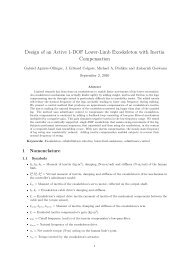
NORTHWESTERN UNIVERSITY
PASSIVE IMPLEMENTATION OF MULTIBODY SIMULATIONS
FOR HAPTIC DISPLAY
A DISSERTATION
SUBMITTED TO THE GRADUATE SCHOOL
IN PARTIAL FULFILLMENT OF THE REQUIREMENTS
for the Degree
DOCTOR OF PHILOSOPHY
Field of Mechanical Engineering
by
J. Michael Brown
EVANSTON, ILLINOIS
December 1998

ABSTRACT
PASSIVE IMPLEMENTATION OF MULTIBODY SIMULATIONS
FOR HAPTIC DISPLAY
J. Michael Brown
The development of complex virtual environment simulations is a challenging
problem in haptic display. Due to the dynamic interactions between the human operator,
mechanism, sensors, actuators and physics-based simulation, provision of stability
guarantees is both an interesting theoretical question and an important practical concern.
Most existing virtual environments rely on the careful tuning of environment and control
parameters to ensure stability. Whenever changes are made to the environment (such as
changing the length of an object), these parameters have to be re-tuned. While merely
annoying for relatively simple environments, this process becomes impractical for
complex ones.
The focus of this work is the development of a software architecture that permits
the simulation of complex multibody environments on a haptic display. This architecture
separates the haptic display from the simulation, such that stability of the haptic display is
not strongly dependent on simulation parameters. These simulations exhibit vastly
improved stability properties compared to previous implementations. Since the haptic
display and virtual environment are still weakly connected, guidelines for the design of
virtual environments are presented.
ii

Specifically, this thesis presents four distinct results associated with the proposed
software architecture. The first result is a detailed passivity analysis of a 1 degree of
freedom haptic display, generalizing previous analyses and providing design guidelines
for the proposed software architecture. This result also substantiates discrete-time
passivity as an exemplar for physics-based simulation methods. The second result is the
establishment of a connection between the incremental conservation properties of
physics-based numerical methods and discrete-time passivity of their numerical
operators. This connection has important implications about which numerical methods
are appropriate for use with haptic displays. The third result shows that discrete-time
passive numerical operators require the solution of implicit equations. For reasons that
are discussed, implicit equations are usually not solvable in real-time, making them
difficult to use with haptic displays. The final result is an improved tuning procedure that
preserves device passivity even with numerical methods that are not discrete-time
passive.
iii

ACKNOWLEDGMENTS
Top billing goes to my advisor, Ed Colgate, for providing me with an
environment where I was allowed the freedom to roam. Because of this freedom, I have
been forced to take more responsibility for myself and for the others around me. I've
learned a lot about haptic displays and control, but I've learned a lot more about all sorts
of other things, from teaching to writing to balancing family life with work.
Several other people deserve specific mention for their contributions to the work.
Beeling Chang, whom I've had the pleasure to work alongside for almost six years,
showed that the theory contained in this document is worthwhile by actually putting it
into practice. Brian Miller, despite his recent arrival in the lab, caught up quickly, and
has been invaluable in figuring out some of the more difficult concepts. He also played
the important role of proofreader for much of this document. Brent Gillespie also took on
this role, as well as providing all sorts of useful advice. Paul Millman left his fingerprints
on much of the hardware in our lab, and because of that, it all still works. I would like to
thanks the members of my doctoral committee -- Michael Peshkin, Scott Delp, and Randy
Freeman -- for making sure that this document is technically sound and relevant. Finally,
I would like to acknowledge Northwestern University's Cabell and Nugent Fellowship
Programs, as well as the NASA Graduate Student Researchers Program, for providing
financial support in the past six years.
On a personal level, I want to thank all the members of the Laboratory for
Intelligent Mechanical Systems (and Social Policy?) for keeping things interesting,
especially in the dog days of writing this document. Special thanks go to Carl Moore,
who is constantly forcing me change the way I think about the world and my place within
iv

it. Exalted Webmaster Bernie Reger has been a good friend and confidant ever since a
fluids class many years ago. I'm also indebted to Witaya Wannasuphoprasit, Mike
βrokowski, Don Cantrell, Andy Lorenz, Jon Lea, Julio Santos-Munné, Aaron Mills and
Sang An for their friendship and counsel at various points in past several years.
Finally I'd like to thank my parents and sister for supporting my efforts for as long
as I can remember, as well as Mick and Joan Howard for all their encouragement. Most
of all, I want to thank Jodi for seven years of the best friendship I could ever hope for,
and for teaching me that a life lived in fear is a life half-lived.
v

CONTENTS
Chapter 1
Introduction ..................................................................................................................... 1
1.1 Background .................................................................................................. 1
1.2 State of the art .............................................................................................. 3
1.3 Goals of the work ......................................................................................... 4
1.4 Contributions................................................................................................ 6
1.5 Organization of the document...................................................................... 7
Chapter 2
Review of sampled-data systems and passivity .............................................................. 9
2.1 Sampled-data systems .................................................................................. 9
2.2 Basic passivity definitions, examples, and theory ....................................... 13
2.2.1 Continuous-time systems .............................................................. 14
2.2.2 Discrete-time systems ................................................................... 15
2.2.3 Stability of coupled systems ......................................................... 16
Chapter 3
Review of previous passivity analyses of haptic displays .............................................. 18
3.1 Passivity of virtual environments with linear dynamics .............................. 19
3.2 Passivity of environments with a virtual coupling and linear dynamics...... 24
Chapter 4
Passive implementations of haptic virtual environments................................................ 29
4.1 Generalized two-port virtual coupling ......................................................... 29
4.2 Admittance causality virtual environments.................................................. 35
4.3 Impedance causality virtual environments................................................... 40
Chapter 5
Discrete-time passivity of physics-based numerical methods ........................................ 43
5.1 Performance evaluation for physics-based numerical methods ................... 45
5.2 Incremental discrete-time passivity ............................................................. 46
5.3 Discrete-time passive numerical integration of a 1 DOF particle................ 48
5.4 Discrete-time passive numerical integration of a 2 DOF particle................ 55
5.5 Discrete-time passive numerical integration of a rigid body in space ......... 58
5.6 Discrete-time passive collision response ..................................................... 64
5.6.1 Basic concepts of unilateral constraints ........................................ 65
5.6.2 Energy conserving collision response........................................... 67
5.6.3 Discrete-time passive collision response ...................................... 70
Chapter 6
Implicit vs. explicit formulations .................................................................................... 72
6.1 Delayed vs. non-delayed integrators - real time implementation ................ 72
6.2 Delayed vs. non-delayed integrators - discrete time passivity..................... 76
vi

Chapter 7
Minimum mass for haptic display simulations ............................................................... 80
7.1 Haptic display passivity with delayed numerical integrators....................... 80
7.2 An improved tuning procedure .................................................................... 92
7.3 Extension to multibody simulations............................................................. 96
Chapter 8
Conclusions and future work .......................................................................................... 98
References ...................................................................................................................... 101
Vita ................................................................................................................................. 105
vii

CHAPTER 1
INTRODUCTION
This thesis involves the development of stable virtual environment simulations for
haptic interfaces. A haptic interface comprises an input/output device (such as a forcefeedback
joystick or exoskeleton), a real-time controller, and a real-time simulation of a
virtual environment. The controller collects information from the input/output device's
sensors (position, velocity, force, and torque are the most common), which are then used
as inputs to the simulation. The simulation estimates the forces the user should feel based
on these sensor values and the internal state of the simulation itself. The simulation
outputs are used by the controller to drive the input/output device's actuators. This type
of system allows users to touch, feel, and manipulate virtual environments.
1.1 Background
Virtual reality in general, and haptic interface in particular, are driven by the
desire for human interaction with various types of simulations. Depending on the
purpose of the interaction, most applications fall within one of four major categories:
training, manipulation, communication, and entertainment. Training applications include
aeronautical (Colgate, et al. 1995) and surgical training (Basdogan, et al. 1998,
Baumann, et al. 1996, Cotin, et al. 1996, Gibson, et al. 1996), rehabilitation (Hogan, et al.
1992), and education (Brooks, et al. 1990). The fundamental goal of the interaction is to
1

2
allow the user to practice and learn in a safe, structured environment, perhaps providing
haptic guidance along the way. Manipulation applications are centered around enhancing
a user's ability to understand and control digitally stored information. Applications range
from virtual prototyping (Nahvi, et al. 1998) and design (Stewart, et al. 1997) to novel
user interfaces for commercial operating systems (e.g., Immersion Corporation's
FEELIt mouse). In communication, two users are brought to a shared virtual
environment (Buttolo, et al. 1996), or a single user manipulates a remote scene with the
help of virtual fixtures (Rosenberg 1993). Entertainment applications take aspects of all
three categories above, but the final goal is to provide enjoyment to the user, rather than
to accomplish some commercially or socially motivated task. A separate non-commercial
use of haptic displays is fundamental research into pyschophysics and human motion
control (Durlach and Mavor 1994), which produces results that are important for all of
the above applications.
Vision-based interaction, while quite useful for many applications, is sometimes
insufficient to give the user a sense of immersion in the virtual environment. Certain
simulations require sound to be effective, while others require haptic sensations. For
example, if a medical student is learning how to perform a lumbar puncture, how the
needle insertion feels is an important part of the task (Bostrom, et al. 1993). In training
tasks in general, if the task to be learned requires manual dexterity or relies on haptic
cues, then a haptic interface may enhance the training. In manipulation and
communication tasks, the addition of haptic components can form a more natural
interface to the virtual and remote environments. For example, in three dimensional
CAD systems, it has been theorized that allowing a designer to interact haptically with an
environment will enhance his or her ability to manipulate that environment (Hollerbach,

3
et al. 1997). In entertainment applications, anecdotal evidence suggests that haptic
interfaces are "cool", so that adding haptic sensations may improve their marketability.
1.2 State of the art
Many of the proposed applications for haptic interfaces involve the simulation of
a complex dynamic system. This simulation must then be connected to a haptic display
so that information about forces and motions can be exchanged haptically between the
human user and the virtual environment. At the beginning of this project, however,
virtual environments from published works had consisted primarily of haptic primitives,
like virtual walls (Colgate, et al. 1993, Salcudean and Vlaar 1994) and simple textures
(Howe and Cutkosky 1993, Klatzky, et al. 1989, Minsky 1995). Other implementations
include (Zilles and Salisbury 1995), which describes an approach to point interaction with
complex static environments, but does not address the extension to dynamic
environments. Gillespie (Gillespie 1996) describes the implementation of complex
dynamic environments whose constraint configurations are known a priori.
Notably missing from the haptics literature are general approaches to the interface
between a haptic display and a complex dynamic simulation. This gap can be at least
partially explained by the difficulty of providing stability guarantees when working with
haptic virtual environments. These guarantees are important both because instabilities are
potentially dangerous and because they typically destroy the user's sense of immersion.
Most existing virtual environments rely on the careful tuning of environment and control
parameters to ensure stability. Whenever changes are made to the environment (such as

4
changing the length of an object), these parameters have to be re-tuned. While merely
annoying for relatively simple environments, this process becomes impractical for
complex ones. Additionally, current simulations are designed for a particular haptic
display, and significant work is required to port the simulation over to a new device. As
simulations become more complicated, perhaps being developed for multiple hardware
configurations, this lack of portability becomes more important. Recent work by Adams
et. al. (Adams and Hannaford 1998, Adams, et al. 1998) also addresses these issues, and
in much the same spirit as the present work.
1.3 Goals of the work
As an avenue for exploring this topic, our group has begun developing hand tool
simulations for use in aeronautical training systems. To help motivate this application,
consider the recent use of virtual reality (VR) methods to train Space Shuttle support
personnel in procedures involving highly specialized hand tools. While some tools used
in micro-gravity are quite ordinary, others have unusual shapes and functions (e.g.,
various tools for emergency repairs). In the current VR training environment, tools are
not represented at all, since this inclusion would require simulation of the interactions
between virtual objects. For example, one merely points to a bolt that needs to be
loosened, and it loosens itself. Clearly, this type of environment is useful for learning a
complicated procedure, but not a physical skill. To develop a physical skill, haptic

5
In light of the hand-tool-based environments we envision building, a general
multibody simulation incorporates the required range of physical behaviors. Further, a
simulation of this type would also be useful in virtual prototyping, and may form the
basis for additional applications. Multibody simulations typically address at least a
subset of the following characteristics:
• An environment comprising rigid polyhedra, springs, and dampers
• Bilateral (i.e. permanent) constraints, such as revolute and prismatic joints
• Unilateral constraints, such as collisions, sliding contact or rolling contact
In the effort to build complex multibody environments for haptic interface, a
natural starting point is the physics-based simulation literature, where there have been
countless publications covering the topics of numerical integration, collision detection,
and collision response. This literature pulls from several different research communities:
computer graphics, robotics, and applied mechanics. In recent years, it has produced a
variety of modeling and implementation tools for use with multibody computer
simulations. However, since these tools were not designed with haptic interface in mind,
it is not clear that they will work properly when used in this context. For a review of
multibody simulation formalisms and their applicability to haptic interface, see (Gillespie
1997).
Our own experience has indicated that algorithms which work well with standalone
simulations often fail when implemented with a haptic display. The cause of this
failure is the difficulty of obtaining stability guarantees for any usefully broad class of
environments. To address this difficulty, it would be useful to develop a general-purpose

6
software and hardware architecture for real-time haptic interaction between users and
complex dynamic simulations. Ideally, this architecture would decouple the haptic
display from the multibody simulation, such that stability of the haptic display is not
strongly dependent on simulation parameters. Our goal is to allow a knowledgeable user
(but not an expert in haptic display) to design virtual environments while maintaining
confidence that the resultant system will be stable.
1.4 Contributions
In general terms, the contribution of the present work is the development of a
general-purpose software architecture for real-time haptic interaction between users and
complex dynamic simulations. This architecture separates the haptic display from the
simulation, such that stability of the haptic display is not strongly dependent on
simulation parameters. The separation also allows the simulation software to be ported
easily from one device to another. Since the haptic display and virtual environment are
still weakly connected, guidelines for the design of virtual environments are presented.
Specifically, this thesis makes four significant contributions to the field of haptic
interface. The first is a detailed passivity analysis of a haptic display, generalizing
previous analyses and providing design guidelines for the proposed software architecture.
It also substantiates discrete-time passivity as an exemplar for physics-based simulation
methods. The second contribution of the work is the establishment of a connection
between discrete-time passivity and the incremental conservation properties of physicsbased
numerical methods. This connection has important implications about which

7
numerical methods are appropriate for use with haptic displays. The third contribution of
the work somewhat weakens the first - it is shown that discrete-time passive numerical
operators require the solution of implicit equations. For reasons that will be discussed,
implicit equations are usually not solvable in real-time, making them difficult to use with
haptic displays. The final contribution is that, given restrictions on environment
parameters, device passivity can sometimes be preserved even when using numerical
methods that are not discrete-time passive. An important benchmark simulation is that of
a point mass, and these restrictions take the form of a minimum mass that can be
simulated passively. This development suggests a tuning procedure that can be used to
guarantee stability over a wide range of virtual environments.
1.5 Organization of the document
Chapter 2 contains a selective review of terminology and basic theory associated
with the passivity of sampled-data systems, and Chapter 3 reviews previous passivity
analyses of haptic interfaces. Chapter 4 contains a generalization of prior passivity work,
and provides guidelines for software design. Chapter 5 establishes the connection
between discrete-time passivity and the conservation properties of physics-based
simulation methods. Chapter 6 shows that discrete-time passive operators require the
solution of implicit equations, and discusses why these equations are difficult to use with
haptic displays. Chapter 7 explores the use of numerical methods that are not discretetime
passive, including a derivation of the minimum mass that can be simulated using

8
specific explicit formulations. Finally, Chapter 8 summarizes the results and significance
of the work and discusses some avenues for future research.

CHAPTER 2
REVIEW OF SAMPLED-DATA SYSTEMS
AND PASSIVITY
The first section of this chapter reviews the basic concepts and notation used to
describe the dynamics of sampled-data systems (systems which contain both continuous
and discrete portions). The second section reviews the basic concepts, definitions and
theorems of passivity analysis.
2.1 Sampled-data systems
`
Usually, a sampled-data system has a continuous-time plant (such as a motor),
and a discrete-time controller (e.g. a computer or DSP chip). Conversions from
continuous to discrete time are handled by an A/D converter, or sampler, which transmits
the value of the continuous signal only at discrete (usually periodic) times. Conversions
from discrete back to continuous time are handled by a D/A converter, or "hold" operator,
which holds the discrete numbers over time to produce a continuous signal. The most
common hold operator is a zero order hold (ZOH), which continually outputs the most
recent number passed to its input.
Figure 2.1 shows an example of a sampled-data system with a continuous-time
plant and a discrete-time controller.
9

10
r k Digital
u k Hold
u(t)
Controller Operator
Plant
Dynamics
y(t)
y k
Sampler
Figure 2.1. Diagram of a sampled data system. Continuous functions are represented with f(t),
whereas discrete functions are represented with f k . The computed controller effort, u k , becomes a
continuous signal, u(t), through the hold operator. The plant output, y(t), is sampled, becoming y k .
In addition to the plant output, the digital controller acts on the discrete reference signal r k .
The control effort u(t) and system output y(t) are continuous-time functions, and can be
expressed as solutions of differential equations that represent the dynamics of the
continuous system. The controller output u k , the sampled output y k , and the reference
input r k are discrete-time functions, and can be expressed as solutions of difference
equations that represent the dynamics of the discrete system. It is important to
understand that, in reality, discrete signals exist only as a train of numbers, and that
difference equations operate on these signals without reference to time (i.e., time is a
continuous concept, and is not well-defined in a purely discrete system).
In a sampled data system, however, these discrete signals interact with a
continuous time system via the sample and hold process. In this domain, time does exist,
and in fact is quite important in discussing the performance of the system. Thus, it is
convenient to issue a "time stamp" that expresses when the discrete signals occur
compared to continuous time events. Usually, periodic sampling is used, so we can
express the time stamp as a multiple of the sampling time. Thus, y k corresponds to the

11
value of the output at the time t=kT and u k is the controller output at the same instant of
time.
Figure 2.2 demonstrates how linear continuous-time operators and signals may be
represented with Laplace variables and functions, which encapsulate the frequency
content of signals and linear operators via the Laplace Transform. Linear discrete-time
operators and signals may be represented with pulse variables and functions, which use
the Z-transform to encapsulate frequency content.
r(z) +
u(z) u(s)
H(z)
ZOH
-
y(z)
G(s)
y(s)
T
Figure 2.2. Block diagram of a linear sampled-data system with a zero order hold and periodic
sampling. Continuous functions are represented in the Laplace domain with f(s), and discrete
functions are represented with f(z).
A subtlety is that pulse variables are continuous time representations of discrete signals,
so that while the actual discrete signal u k is defined only at sample times, the pulse
representation u(z) is a series of impulses, each with area u k , separated by a continuous
zero signal (see Figure 2.3). This representation is very convenient for sampled data
systems because linear continuous time effects, like computational delay, can be
mathematically represented in the discrete part of the system. These effects are not easily
modeled using traditional difference equations.

12
(A)
u(k)
x
x
x
x
x
x
x
x
kT
u*(t)
(B)
t
(C)
u ZOH (t)
Figure 2.3. Representations of discrete signals. Original discrete signal (A), pulse variable
description (B), signal after zero order hold (C).
t
Throughout this document, we will use linear models to describe the dynamics of
the continuous-time portions of the system, so Laplace variables and functions will be
sufficient. The discrete portions of our system, however, contain physics-based models
of multibody systems. These models are often non-linear, so we will resort to difference
equation descriptions of this portion of our system when necessary.
Figure 2.4 shows a block diagram representing the dynamics of a generic haptic
display system. The human operator, actuators, mechanism, and sensors form the
continuous-time portion of the system, while the virtual environment constitutes the

13
discrete-time part of the system. The A/D and D/A form the interface between the
continuous and digital domains of this sampled-data system.
Human
Operator
Actuator
Dynamics
+
-
Mechanism
Dynamics
Sensor
Dynamics
Continuous-time
D/A
A/D
Discrete-time
Virtual Environment
Simulation
Figure 2.4. Generic block diagram a haptic display. The human, actuators, mechanism, and
sensors are all continuous-time systems, while the virtual environment is a discrete-time system.
The A/D and D/A form the interface between them. The shaded areas emphasize which parts of
the haptic display are continuous vs. discrete time.
2.2 Basic passivity definitions, examples, and theory
This section reviews some basic concepts, definitions and theorems of passivity
analysis. It is not intended to be a comprehensive introduction to passivity theory, but
rather a very limited introduction to the specific results we will use throughout this
document. A much more rigorous and comprehensive treatment can be found in (Desoer

14
and Vidyasagar 1975, Khalil, et al. 1996). This section is divided into four parts:
continuous-time systems, discrete-time systems, stability of coupled systems, and
sampled-data systems.
2.2.1 Continuous-time systems
In this document, we only treat continuous-time systems that have linear
dynamics, so that while there are powerful passivity tools for dealing with non-linear
continuous-time systems, we will remain focused on the linear ones. Having said this,
consider a generic (possibly non-linear) operator, G, which operates on an input signal,
u(t), resulting in the output signal y(t). An intuitive definition of system passivity is that
the maximum extractable energy be less than or equal to the initial stored energy.
Translating this definition into more mathematical terms requires more information about
the nature of the signals. However, we can make a mathematical statement about
operator passivity without knowing anything about the nature of the signals. This
statement by itself doesn't specify anything about energy, but can be a powerful analytical
tool nonetheless. The operator G will be passive iff:
t
(2.1) ∫ u(t) ⋅ y(t)dt ≥−E(t 0
) ∀ u(t), ∀t ≥ t
t 0
0
where E(t 0 ) is some constant that depends only on the initial conditions of the system.
This mathematical statement of operator passivity matches the energy definition of
system passivity when u(t) and y(t) are complimentary effort/flow variables. In this case,
u(t)·y(t) is the instantaneous power delivered to the system, and G is defined as an

15
impedance operator (i.e., it acts on effort to produce flow or, conversely, flow to produce
effort).
If we further restrict G to be a linear operator, we can then describe it in the
frequency domain via Parseval's Theorem. In this case, (2.1) simplifies to:
(2.2)
Re[Ĝ( jω)] ≥ 0 ∀ ω ∈R
where Ĝ ( jω ) is the frequency-domain description of the operator G. Later in this
section, we will use (2.2) to help generate passivity conditions on the continuous portion
of the system.
2.2.2 Discrete-time systems
As in the previous section, consider a generic (possibly non-linear) operator, G,
which operates on a discrete input signal, u k , resulting in the discrete output signal y k .
Unlike the continuous-time case, we will not try to make an intuitive statement of system
passivity for discrete systems. The problem is that the definition of extractable energy is
arbitrary, even when u k and y k are an effort/flow pair. However, we can make a
mathematical statement about operator passivity - the operator G will be passive iff:
N
(2.3) ∑ u k ⋅ y k ≥−E 0 ∀ u k , ∀ Ν ∈ Ζ +
k=0

16
where E 0 is again a constant dependent on the initial conditions. Since much of our
analysis deals with non-linear discrete-time simulations of dynamic systems, (2.3) will
often be used for determining discrete-time passivity.
If we further restrict G to be a linear operator, we can describe it in the frequency
domain via Parseval's Theorem:
(2.4) Re[ ˜g(e jθ )] ≥ 0 ∀θ ∈ [0, 2π]
where ˜g(e jθ ) is the discrete frequency-domain description of the operator G. It is
important to remember that (2.4) will be of limited usefulness due to the restriction that G
be a linear operator. However, it will be used as a shortcut to (2.3) in several examples
later in this document. Having established the definitions for energetic passivity and
operator passivity for both the continuous-time and the discrete-time cases, we turn to the
Passivity Theorem and its corollaries in order to understand the interactions between
passivity and coupled stability.
2.2.3 Stability of coupled systems
Consider the system shown in Figure 2.5, which shows the coupling of two
(possibly non-linear) systems G and H. The Passivity Theorem states that if G is input
and output strictly passive, but otherwise arbitrary, then a necessary and sufficient

17
u(t)
+
-
G
y(t)
H
Figure 2.5. Block diagram showing the connection of two operators, where G is strictly passive
(but otherwise arbitrary), and H is a system to which it is connected. Signals u(t) and y(t) do not
have to be a complimentary effort/flow pair.
condition for coupled stability is the passivity of H. * This result seems intuitive, since
neither system can continually generate energy needed for unstable oscillations. A
corollary to the theorem is that if G is strictly passive (but otherwise arbitrary), then a
necessary and sufficient condition for the passivity of H is that the coupled system be
guaranteed stable. In practice, however, it is difficult to formulate stability guarantees for
systems containing arbitrary non-linear operators. A direct derivation of passivity
conditions using (2.1) or (2.3) is more appropriate for this type of proof.
If G is a linear passive (but otherwise arbitrary) impedance, then stability of the
coupled system is easier to prove, and this is the approach taken below. It is important to
note, however, that stability of the coupled system provides only a necessary condition
for the passivity of H. Even though the system is stable, H might still be active, but the
linear operator G will have no way of extracting the energy necessary to identify it as
active. If H is linear, then the condition again becomes necessary and sufficient.
* Input and output strict passivity is a slightly more demanding condition than that specified in (2.1) and
(2.3). If the operator in question is linear, then (2.2) and (2.4) apply, but with the left hand side positive and
uniformly bounded away from zero. Throughout this document, stability should be interpreted as finite
gain input/output stability in the 2-norm, unless otherwise specified. Details of these conditions can be
found in (Khalil, et al. 1996).

CHAPTER 3
REVIEW OF PREVIOUS PASSIVITY ANALYSES OF
HAPTIC DISPLAYS
A primary goal of virtual environment simulations, whether haptic or visual, is to
achieve a sense of "presence" in the virtual environment (Slater and Usoh 1993). If the
state of that environment becomes computationally unstable, the sense of presence will be
damaged, if not completely destroyed (imagine if a wrench began oscillating
uncontrollably against a nut). Thus, virtual environment simulations, whether haptic or
visual, need to provide stability guarantees. Our experience has shown that, for haptic
display, stability guarantees are one of the most challenging aspect of virtual environment
implementation.
The difficulty in any traditional stability analysis of this system is the unmodeled
dynamics of the human operator. Even though the virtual environment itself might be
stable, interaction with a human operator via a haptic interface may cause instability. In
our studies of virtual environments, we have had many experiences with human operators
adjusting their own behavior until oscillations resulted. Another approach to proving
robustness is to derive the conditions under which the haptic display handle appears
passive to the human operator. Under these conditions, the device cannot generate
energy continually over time, making actuator-driven instabilities impossible. The
following sections outline past theoretical approaches to achieving this goal.
18

19
3.1 Passivity of virtual environments with linear dynamics
For the past several years, our group has been using passivity as a tool to explore
the performance of haptic displays. The foundation for this work was laid in (Colgate
and Schenkel 1997), which developed necessary and sufficient conditions under which a
haptic display with linear virtual environment dynamics will appear passive. The result
was extended to include the effect of a unilateral constraint operator acting on the
environment. Figure 3.1 shows the system model used in the analysis:
Operator
G * (jω)
u s
1 - e - sT u
s
zero order hold
-
f
-
v
T
1 1
h
ms+b
s
h s
H(z)
Figure 3.1. Colgate and Schenkel's model of a 1 DOF haptic display. Parameters m and b are the
inherent inertia and damping of the haptic display handle. H(z) is the virtual environment, T is the
sample time, h is the handle position and u is the actuator effort (h s and u s after sampling).
With the goal of understanding the effects of inherent manipulandum dynamics
and sample-and-hold on the achievable dynamic range of haptic displays, Colgate and
Schenkel developed a simple model that still captured the salient features of these
components. This model has one degree of freedom and uses an ideal actuator, position

20
sensor, sampler and zero order hold. The model of the mechanism dynamics
approximates the behavior of the 1 DOF device in our laboratory.
The analytical approach was to replace the human operator with an arbitrary linear
time-invariant passive (ALTIP) impedance and then derive the conditions under which
the coupled system had to be stable. According to the Passivity Theorem (see §2.2.3),
stability when connected to an ALTIP impedance provides a necessary and sufficient
condition for the passivity of the haptic display. Insight into the derivation of these
passivity conditions can be obtained graphically through a Nyquist-style analysis. Figure
3.2 shows a progression of transfer function and their corresponding regions in the
Nyquist plane:
Im
Im
Im
Im
Re
b
Re
1
b
Re
Re
Z 0 ( jω)
mjω+b+Z 0 ( jω)
1
mjω+b+Z 0 ( jω)
G * (jω)
Figure 3.2. Graphical representation of passivity derivation. Regions corresponding to the ALTIP
impedance, mechanism, and sample/hold dynamics are shown in the Nyquist plane.
The ALTIP impedance, Z 0 (jω), occupies the entire right half-plane. Through a series of
Möbius transformations * , the effects of additional dynamics are incorporated. Adding
the mass and damping of the mechanism translates the half-plane to the right by the
* A Möbius transformation (also known as a bilinear transformation or a linear fractional transformation) is
a specific type of conformal map, consisting of translations, rotations, magnifications, and inversions. It
has the property that circles and lines always map to circles or lines. Disks, half-planes and holes always
map to disks, half-planes or holes.

21
amount of damping b. Since the desired mapping is from force to velocity, this halfplane
must be inverted, yielding a disk of radius , centered at on the real axis.
1
1
2b 2b
The primary difficulty in this analysis is modeling the effects of sample and hold on the
transfer function from u s to h s . Using the impulse model of sampled systems and the zero
order hold model shown above, G * (s) is given by an infinite series:
(3.1) G * ()= s
1 T
+∞
∑ Gs+jnω ( s )
ω s = 2π T
k=−∞
(3.2) G(s) =
1− e−Ts
s 2 1
ms + b + Z 0 s ()
Because the disk of the previous step is frequency-independent, it can be removed from
the summation in (3.1):
(3.3) G * ()= s
1 T
1
ms + b + Z 0 s
() ⋅ +∞
1−e −Ts+jnω ( s )
∑
k=−∞ ( s + jnω s ) 2
The remaining summation has a closed form, resulting in the following transfer function:
(3.4) G * (jω) = T 2
e −jωT −1
1−cosωT ⋅ 1
mjω+b+Z 0 (jω)
The last term in this expression is the unrotated disk shown in Figure 3.2. The terms in
front are an additional Möbius Transformation, resulting in a scaled and rotated disk. At

22
each frequency, the center and radius of the disk are:
(3.5) Center G * ( jω)
{ }= T e −jωT −1
4b 1− cosωT
(3.6) Radius{ G * ( jω)
}= T 4b
e −jωT −1
1− cosωT
Having fully identified the region, a Möbius Transformation that maps this disk to the
complete interior of the unit disk, pointwise in frequency, can be found. Finally, Colgate
(Colgate 1994) found a related transformation that, when applied to H(z), results in a
system with the same closed loop characteristic equation as the original. The Small Gain
Theorem was then used to obtain necessary conditions for closed loop stability:
(3.7) b > T 2
1
1 − cosωT Re { (1 − z−1 )H(z)} z=e
jωT
0≤ω≤ω N
where ω N =π/T is the Nyquist frequency. An application of Parseval's Theorem was used
to show that (3.7) is also a sufficient condition for closed loop stability of this system.
Finally, it was proved that (3.7) remains unchanged if the virtual environment is preceded
by a unilateral constraint operator.
This result can be used, for example, to investigate one implementation of a
virtual wall:
(3.8) H(z) = K + B T
( 1− z−1)

23
where K is the virtual stiffness and B is the virtual damping. When substituted into (3.7),
the passivity condition simplifies to:
(3.9) b > KT
2 + B
This result is important because it provides design guidelines for the mechanism
dynamics of a haptic display. It shows that increasing the inherent physical damping of
the mechanism will increase the maximum stiffness and damping the device can emulate.
Further, it indicates that negative virtual damping can be used to cancel out the effect of
the added physical damping when the stiffness is zero (i.e., the human operator has
moved outside the wall).
An offshoot of this work was the use of a new performance measure for haptic
displays: the "Z-width" (Colgate and Brown 1994). The Z-width of a haptic display is
the range of impedances that it can simulate passively. This measure can be used to
contrast different devices, even if they have different configurations. It can also be used
along with a measure of simulation quality to compare different implementations of a
given virtual environment. The Z-width is affected by a number of factors, including
inherent mechanism dynamics, controller update rate, and sensor/actuator performance.
To ensure system robustness, the haptic display hardware should never be commanded to
render an impedance that is outside its Z-width.
While quite helpful for providing manipulandum design guidelines, (3.7) is not
usually very effective for designing virtual environments. Along with the restriction to
linear virtual environments, the result doesn't inherently apply to any well-defined class
of virtual environments. Any proposed environment must be substituted into these

24
conditions to see if its implementation will be passive. To move beyond these
difficulties, we need to develop a framework for implementing a wider class of virtual
environments.
3.2 Passivity of environments with a virtual coupling and linear
dynamics
Extension of the virtual wall model to more complicated environments is often
not a trivial task. When a haptic display has both translational and rotational degrees of
freedom, even simple virtual environments generate instabilities if implemented
unwisely. The problem is keeping the device within its Z-width. For example, consider a
peg in hole simulation implemented on a 3-DOF planar haptic display (Figure 3.3).
L
Figure 3.3. Two configurations of a peg in hole simulation. In this implementation, the massless,
perfectly rigid peg tracks the handle of the haptic display. The hole is mechanically grounded and
has a contact stiffness of Kc. The vertical distance between the contact points is L.

25
We can obtain the Z-width of the device either through derivation or experimental
measurement. This Z-width is expressed as a three-element vector [Kx Ky K θ ] T ,
representing the maximum stiffness implementable across the entire workspace
(neglecting for now the role of virtual damping). One approach to keeping the hardware
within its Z-width is to model the peg as a massless rigid body that tracks the handle of
the haptic display, while the hole is compliant. If the peg penetrates any surface, a
reaction force/torque about the center of mass is computed according to the contact
stiffness, Kc, and applied to the handle. In the second configuration of Figure 3.3, the
stiffness matrix of the peg (and thus the handle of the haptic display) is given by:
⎡
K
⎤
⎢ c ⎥
(3.10) K peg = ⎢ 0 ⎥
⎢1
2 K ⎥
c
⎣⎢
L2
⎦⎥
There are two problems that make this approach infeasible. First, the rotational and
translational components of the stiffness are interdependent (i.e., typically only one
component can be set to its maximum stiffness for a given simulation). The other
component will either be too compliant or exceed the Z-width of the device. Second, the
stability of this simulation is geometry-dependent. For a given contact stiffness, it is
always possible to choose a peg length that will result in severe instability. This second
problem becomes even worse as simulations become more complicated, due to the
increase in the number of parameters that strongly affect stability. A successful
implementation needs to utilize the full Z-width of the device, while maintaining stability

26
independent of simulation geometry. Finally, simulations in this framework must be
designed for a particular device, resulting in poor simulation portability.
In (Colgate, et al. 1995), a more general approach to the implementation of
complex virtual environments was developed. While the analysis was restricted to
environments with linear dynamics, an important new concept was incorporated: the
virtual coupling. Shown in Figure 3.4 as a spring and damper, the virtual coupling allows
the environment design to be separated from the sampled-data control issues associated
with haptic display. The virtual coupling is a multi-dimensional compliant element that
is placed between the haptic display hardware and the virtual tool. Acting as an
impedance filter, the virtual coupling limits the rendered impedances to within the Z-
width of the particular device being used. If the virtual environment calls for an infinite
stiffness to be displayed, such as when a rigid wrench interacts with a rigid bolt, the
device will instead render the impedance of the virtual coupling.
operator
"Virtual Coupling"
K
B
haptic display
Discrete-time Passive
Simulation
Figure 3.4. Conceptualization of a virtual coupling in a hand tool simulation.

27
The 1 DOF model shown in Figure 3.5 was used to demonstrate the effectiveness of this
approach. In this model, the virtual coupling is a 2-port operator, where each element
contains a backwards difference discretization of a spring-damper.
Operator
f v
1 - e - sT u -
- 1 1
s
ms+b
s
zero order hold
F 1 (z)
x 1 (z)
T
x
F 2 (z)
C(z)
v 2 (z)
E(z)
Figure 3.5. Block diagram of a 1 DOF haptic display using a virtual coupling. The virtual coupling
and environment are represented by C(z) and E(z), respectively. The human operator, as in
previous work, is replaced with an arbitrary linear time-invariant passive operator.
The mappings go from endpoint position and virtual environment velocity to force, with
the two forces being equal and opposite because they represent the force between the
haptic display handle and virtual environment.
(3.11)
( )
( )
⎡
⎡F 1 (z) ⎤
K + B 1− z−1
⎢
⎣F 2 (z) ⎥
⎦
= ⎢ T
⎢
⎢−K − B ⎣ T 1 − z−1
−KT
1 − z −1 − B ⎤
⎥⎡x 1 (z) ⎤
KT
1 − z −1 + B ⎥⎢v ⎥⎣
2 (z) ⎥
⎦
⎦

28
Using structured singular values, it was demonstrated that the conditions under which this
system is stable are the same as for the virtual wall (3.9). This result is useful because it
extends the virtual wall result to a significantly wider class of virtual environments --
those with linear discrete-time passive dynamics.
The scope of the result is limited, however, because the analysis applies only to
the particular virtual coupling given in (3.9). It would be preferable to have a more
general result like (3.5), which could then be used as a tool for designing both virtual
couplings and environments. A second limitation is the analysis only addresses
simulations with linear dynamics, whereas many of the systems we wish to simulate are
highly non-linear. The final limitation is that the output of a numerical simulation is
likely to contain position information, while the analysis above assumes velocity is the
output. The next chapter presents a generalized version of the virtual coupling, and will
address the issues mentioned above.

CHAPTER 4
PASSIVE IMPLEMENTATIONS OF HAPTIC VIRTUAL
ENVIRONMENTS
The developments that follow will continue to use the virtual coupling to allow
the passive implementation of a broad class of virtual environments. Section 4.1 provides
the most general passivity analysis, with an arbitrary linear two-port virtual coupling.
The primary result is a derivation of the conditions under which a haptic display will be
passive given any linear two-port virtual coupling. Sections 4.2 and 4.3 explore two
physically motivated special cases of the general theory. These special cases allow
simpler and more useful passivity conditions to be developed. Section 4.2 specifically
addresses admittance causality virtual environments, while §4.3 deals with impedance
causality.
4.1 Generalized two-port virtual coupling
In this section, we return to the passivity tools developed in (Colgate and
Schenkel 1997), extending them to include a general two-port linear virtual coupling.
The goal of the analysis is to derive the conditions under which the haptic display will
present a passive impedance to the human operator. Figure 4.1 shows a two-port virtual
coupling implementation of a 1 DOF haptic display. As in §3.1, haptic display passivity
29

30
conditions are derived by demonstrating stability when the human operator is replaced by
an arbitrary linear time-invariant passive (ALTIP) impedance.
f human
Human
Operator
G * (jω)
f h
1 − e − sT
s
+
-
1
ms + b
v h
1
s
T
x h
-
C 11
( z) C 12
() z
C 21
() z C 22
() z
-
s 1
s 2
Simulation
passive operator
Figure 4.1. Model of a haptic display with a two-port virtual coupling. G*(jω) represents the
dynamics of the sample/hold, mechanism, and human operator, x h is the measured position of the
haptic display handle, while f h is the force to be applied to the mechanism by the actuators.
Signals s 1 and s 2 are the inputs and outputs of the simulation, and are not required to be specified
for the analysis.
The pulse transfer function of the virtual coupling maps x h and s 2 into f h and s 1 :
(4.1)
()
⎡−f h z ⎤
⎢
⎣s 1 () z ⎦
⎥ = ⎡ C11 z
⎢
⎣C 21 z
() C 12 z
() C 22 () z
x h
⎤⎡
⎤
⎥⎢
⎦⎣−s⎥
2 ⎦

31
It is assumed that the environment simulation is discrete-time passive (i.e., the
mapping from s 1 to s 2 is a passive one according to (2.3) or (2.4)). The model of the
continuous portion of the system and the virtual coupling is the same as that used in §3.1.
The goal of this analysis is to develop conditions under which the mapping from s 2 to s 1 ,
via the virtual coupling and G * (jω), is a passive one. These conditions will be sufficient
to establish the stability of the entire system, and necessary to establish the passivity of
the haptic display.
As in the previous chapter, we model the continuous-time dynamics and the
sample-and-hold using the techniques developed in (Colgate and Schenkel 1997). Recall
that G * (jω) captures the dynamics of the mechanism, the ALTIP impedance that replaces
the human operator, and the sample/hold operators:
(4.2) G * ( jω) = T 2
e − jωT −1
1 − cosωT ⋅ 1
mjω + b + Z 0
( jω)
where T is the sample time, m is the mechanism inertia, b is the mechanism damping, and
Z 0 (jω) is the ALTIP impedance. The region associated with G * (jω) is a disk whose edge
passes through the origin, and whose center and radius are:
(4.3) Center G * ( jω)
{ }= T e −jωT −1
4b 1− cosωT
(4.4) Radius{ G * ( jω)
}= T 4b
e −jωT −1
1− cosωT

32
Further manipulations can be performed on G * (jω) through the continued use of Möbius
transformations and block diagram manipulation. The transfer function from -s 2 to s 1 is
calculated directly, resulting in the standard coupled stability form shown in Figure 4.2.
G ' (jω)
s 1
-
Simulation
s 2
passive operator
Figure 4.2. Coupled stability form of haptic display system. The mechanism, ALTIP impedance,
sample/hold, and two-port virtual coupling dynamics are contained in G'(jω). The virtual
environment is restricted to be discrete time passive.
The mechanism, ALTIP impedance, sample/hold and virtual coupling dynamics are
contained in G'(jω):
( )
()
(4.5) G ' (jω) = −C 12 ()⋅C z 21 ()⋅G* z jω
1+C 11 ()⋅G z
* z
+C 22 () z
z=e jωT
The virtual environment is passive, but otherwise arbitrary, so a necessary and sufficient
condition for system stability is the strict passivity of G'(jω). Since G'(jω) is a frequencydependent
region in the complex plane, the Passivity Theorem (2.2) can be used to

33
demonstrate strict passivity:
(4.6) Re{ G' (jω)}>0
Equivalently, the inverse of G'(jω) should also have a positive real part:
⎧ 1 ⎫
(4.7) Re⎨
⎬>0
⎩G'(jω)
⎭
Substituting (4.5) into (4.6) and (4.7), respectively, yields two equivalent passivity
conditions for the haptic display:
( )
⎧
(4.8) Re −C 12 ()⋅C z 21 ()⋅G* z jω
⎨
⎩ 1+C 11 ()⋅G z
* () z
⎫
+C 22 () z ⎬
⎭ z=e
jωT
>0
⎧⎪
1 + C
(4.9) Re
11 ()⋅G z
* z
⎫⎪
⎨
[ C 11 ()⋅C z 22 ()−C z 12 ()⋅C z 21 () z ]⋅G * ⎬
⎩⎪
( jω)+C 22 () z
()
⎭⎪ z=e
jωT
>0
For any given virtual coupling, (4.8) or (4.9) can be evaluated to determine the passivity
conditions for the haptic display. The difficulty here is in forming a useful analytic result
for the general case. Since G*(jω) is a disk in the complex plane, its inverse can be a
half-plane, a hole, or another disk, depending on whether G*(jω) touches, encompasses,
or misses the origin, respectively. Additionally, G*(jω) appears in both the numerator
and denominator of both (4.8) and (4.9), making it impossible to simplify the results
further without specifying something about the virtual coupling.

34
It is interesting to compare this formulation with that used in (Adams and
Hannaford 1998). Adams and Hannaford address the same issues, and in a very similar
spirit to the present work. Using a "virtual coupling network", they develop conditions
under which a model of a 1 DOF haptic display running a discrete-time passive
environment will present a passive impedance to the human operator. The difference
between the two formulations is that Adams and Hannaford perform their analysis in
discrete time, whereas the present work analyzes the system in continuous time. To
analyze a haptic display model in discrete time, both the mechanism and the sample/hold
dynamics must be discretized, using any of a variety of techniques. Adams and
Hannaford chose Tustin's method to discretize the mechanism dynamics because this
method preserves the passivity properties of the operator. They approximated the
dynamics of the zero order hold with a digital low-pass filter:
(4.10) ZOH()≅ z
1 ( )
2 1+z−1
This filter has unity steady-state gain and 90˚ phase lag at the Nyquist frequency.
Because their model of the sample-hold process is much simpler than the one used in the
present work, broader results were obtained. It is unclear, however, whether the
simplified model of sample-hold significantly compromises the accuracy of the results.
The next section considers a physically motivated special case that will allow for
more useful results to be obtained.

35
4.2 Admittance causality virtual environments
Consider the restriction of the virtual environment to admittance causality (i.e.,
force inputs produce motion outputs). This causality requires s 1 to be a force, since it is
the input for the virtual environment. We can further restrict the virtual coupling by
requiring it to obey Newton's Third Law, so that the force applied to the haptic display by
the actuators is also applied to the virtual environment, but with the opposite sense. With
these two restrictions, a one-port representation is adequate to represent the dynamics of
the system:
f human
Human
Operator
G * (jω)
1 − e −sT
s
-
T
1
1
+ ms + b v h
s
x h
-
f h
C(z)
-
Simulation
x e
1 − z −1
∆x e
+
x e
1
1 − z −1
passive operator
Figure 4.3. Model of a haptic display with a one-port virtual coupling and an admittance causality
virtual environment. Note that the simulation outputs position, rather than velocity.

36
Special care has been taken to use position as the output for the simulation, as the
numerical effects of integration are an important part of the passivity/stability
characteristics of the system. A more realistic model feeds back both position and
velocity, since this approach is typically taken in practice. However, this improved
model does not lend itself to a straight forward passivity analysis due to the mismatch in
the number of inputs and outputs.
For reasons that will be explained in Chapter 5, passivity conditions for physicsbased
simulations are developed using force and position change as the inputs and
outputs, even though the true output of the simulation is position. The 1-z -1 and 1/(1-z -1 )
that follow the simulation are a mathematical construct that permit the analysis to
continue, but have no overall effect on the dynamics of the system. Their difference
equations are never actually used in the simulation. From this point, the development
parallels that of the previous section, as G*(jω) is still given by (3.4). The block diagram
now simplifies to the standard coupled stability form shown in Figure 4.4.
The transfer function from ∆x e to f h and its inverse are calculated directly through
block diagram manipulation and Möbius transformations:
()
(4.11) G ' (jω) = f h z
∆x e z
() z=e
jωT
Cz ()
=
( 1−z −1
)1+Cz ()⋅G * (jω)
[ ] z=e
jωT
(4.12)
1
G ' (jω) = 1−z−1
Cz
()
+1−z ( −1
)⋅G * (jω)
z=e jωT
As in the two-port case, a necessary and sufficient condition for system stability is the
strict passivity of G'(jω). Since G * (jω) is a disk and the Möbius transformations in (4.12)

37
G ' (jω)
f h
Simulation
1 − z −1 -
∆x e
passive operator
Figure 4.4. Coupled stability form of haptic display system. The mechanism, ALTIP impedance,
sample/hold, and one-port virtual coupling dynamics are contained in G'(jω). The virtual
environment is restricted to be discrete time passive.
are not inversions,
1
G'(jω)
c'(jω) and |r'(jω)|, respectively:
will also be a disk. The center and radius will be given by
(4.13) c' ( jω) = T cosωT − jsinωT
2b ( )+1−e−jωT
(4.14) r'(jω) = T 2b
( )
Ce jωT
In order for G'(jω) to be passive, every point in the disk that covers
1
G'(jω)
must have
real part greater than zero. In terms of the center and radius, the real part of the center
must be greater than the radius:
(4.15) Re{ c'(jω) }> r'(jω)

38
Substituting (4.13) and (4.14) into (4.15), we obtain the conditions under which G'(jω)
will be passive and the entire haptic display will be guaranteed stable:
(4.16) b > T 2
1 − cosωT
⎧ jωT
⎪1 − e− ⎫⎪
Re⎨
⎩⎪ Ce ( jωT ⎬
) ⎭⎪
This result is useful because it permits comparison between the effectiveness of different
virtual couplings that might be used with admittance causality virtual environments.
As an example, consider the spring and damper coupling implementation
mentioned previously, whose continuous-time transfer function is given by:
(4.17) Cs ()=K+Bs
where K and B are the virtual stiffness and damping. The discrete version of this transfer
function depends on the mapping used between continuous and discrete time and on the
sample time T. For example, we can calculate the discrete-time transfer functions for a
backwards difference and Tustin’s mapping, respectively:
(4.18) C BD ()=K+ z
B ( )
T 1−z−1
(4.19) C Tustin ()=K+ z
2B T
⎛1− z −1 ⎞
⎜
⎝1+ z −1 ⎟
⎠

39
Substitution of (4.17) and (4.18) into (4.15) yields two different passivity conditions for
the two different virtual couplings. For the spring/damper using the backwards
difference, the passivity condition for the haptic display is the same as that found
previously:
(4.20) b > KT
2 + B
This result indicates that for a given mechanism damping level and simulation update
rate, the virtual stiffness and damping of the coupling can be chosen such that any
discrete-time passive simulation will meet necessary conditions for device passivity. The
simulation can be based on any physics-based modeling technique, whether linear or nonlinear,
as long as it obeys discrete-time passivity. By comparison, the passivity condition
for the spring/damper using Tustin’s mapping is:
(4.21) b >
⎛ KT
⎝ 2 + B ⎞ 1 + 2λ cosωT +λ 2
⎠ 21+cosωT ( )1+2λcosωT
( )
λ=
KT − 2B
KT + 2B
This expression indicates that infinite physical damping is necessary at the Nyquist
frequency, making (4.19) a poor candidate for a virtual coupling for certain passive
virtual environments. Optimization of the virtual coupling is the subject of current and
future work. To date, however, no published works have documented significantly
improved performance over the backwards difference spring-damper virtual coupling
mentioned above.

40
4.3 Impedance causality virtual environments
In this section, we consider the restriction of the virtual environment to impedance
causality (i.e., motion inputs produce force outputs). While probably not the optimal
formulation for multibody systems, impedance environments have been used in many
simulations. Adams and Hannaford (Adams, et al. 1998) showed that any virtual
coupling used with admittance environments can be used with impedance environments
as well, albeit with a slightly different implementation in software.
Returning to the two-port structure of Figure 4.1, this causality requires s 2 to be a
force, since it is the output of the virtual environment. As in the previous section, we can
further restrict the virtual coupling by requiring it to obey Newton's Third Law, so that
the virtual environment's output force is sent directly to the haptic display's actuators, but
with the opposite sense. With these restrictions, a one-port representation is adequate to
represent the dynamics of the system.
As in the admittance causality case, the 1-z -1 and 1/(1-z -1 ) operators are a
mathematical construct and are not implemented in actual simulations. The transfer
function from -f e to ∆x e (via the virtual coupling and G * (jω)) is calculated directly
through block diagram manipulation:
()
(4.22) G ' (jω) = ∆x e z
−f e z
() z=e
jωT
=1−z ( −1
)⋅G * ( jω)+ 1−z−1
Cz
() z=e
jωT
which is the inverse of G'(jω) in the admittance case.

41
f human
Human
Operator
G * (jω)
f h
1 − e −sT
s
-
T
1
1
+ ms + b v h
s
x h
f e
-
Simulation
x e
1 − z −1 1 − z −1
1
-
+
Cz ()
1 ∆x e
x e
passive operator
Figure 4.5. Impedance causality virtual environment with one-port virtual coupling. The virtual
coupling, C(z), is the same as that used for admittance environments.
As a result, the passivity conditions remain the same as in the admittance case.
(4.23) b > T 2
1 − cosωT
⎧ jωT
⎪1 − e− ⎫⎪
Re⎨
⎩⎪ Ce ( jωT ⎬
) ⎭⎪
As in the previous case, this result is helpful because it permits comparison between the
effectiveness of different virtual couplings that might be used with impedance causality
virtual environments. The remainder of the document, however, will focus on admittance

42
causality virtual environments because they seem to be better suited for multibody
simulations.
The use of a virtual coupling like the backwards-difference damped spring allows
the designer to focus on multibody simulation rather than sampled-data stability issues.
The only requirement, from a passivity point of view, is that the numerical methods in the
simulation be discrete-time passive. This change in focus is desirable because discretetime
passivity has a meaningful interpretation when dealing with physics-based
numerical methods. The next chapter explores this issue in greater depth.

CHAPTER 5
DISCRETE-TIME PASSIVITY OF PHYSICS-BASED
NUMERICAL METHODS
In the analyses of the previous two chapters, it was assumed, without explanation,
that the simulation obeys the property of discrete-time passivity. This chapter
investigates the connection between discrete-time passivity and the conservation
properties of the numerical methods used in multibody simulations. The general
contribution of the chapter is to show that if a numerical method meets a specific energy
conservation guideline, it will be discrete-time passive. This result establishes, in the
context of physics-based simulations, guidelines for numerical operators so that they can
then be used with a properly designed virtual coupling to create extremely robust
multibody simulations for haptic display.
Admittance causality physics-based simulations begin with a force input (in this
case from the virtual coupling). From this point, a multibody simulation consists of five
distinct modules: bilateral constraint formulation, integration, collision detection, contact
point determination, and collision response. These modules are together responsible for
advancing the state of the simulation through time and computing the forces that are fed
back to the human operator through the virtual coupling and haptic display hardware.
They must be able to enforce constraints, detect collisions between bodies, and respond to
them in a physically meaningful manner.
43

44
For even moderately complicated environments, the most computationally
intensive module is collision detection, and improving the efficiency of these algorithms
is currently an extremely active area of research (for a survey, see (Lin and Gottschalk
1998)). However, it will suffice for this document to say that collision detection should
be as fast as possible, because computational delay tends to compromise passivity. For
additional detail regarding collision detection and contact point determination for haptic
display, see (Chang 1998).
The subtleties of numerical integration and collision response, however, merit
closer investigation. Their effect on discrete-time passivity can be quite pronounced,
even though they are not a severe computational burden compared to collision detection.
§5.1 discusses in general terms the different methods for evaluating the performance of
numerical integrators used in real-time simulations for haptic display. §5.2 presents the
most general result, an incremental energy conservation principle that guarantees
discrete-time passivity of numerical operators. This conservation principle can be applied
to any physics-based numerical method, regardless of the types of models used in the
environment. §5.3 explores a simple example, a particle constrained to a line. It is
shown that the conservation principle of the previous section has a meaningful physical
interpretation, and can be used to design discrete-time passive numerical integrators.
§5.4 and §5.5 extend the analysis to a particle in a plane and a rigid body in space,
respectively, while §5.6 further extends the results to include collision models between
rigid bodies.

45
5.1 Performance evaluation for physics-based numerical methods
When modeling complex dynamic systems, the result is typically a set of nonlinear
differential equations with no known analytic solution. Often, researchers must
resort to using a numerical method to approximate the solution to this set of equations.
There is no "best" way to approach this task in general, and a vast research literature has
developed which explores different approaches for a wide variety of applications. In our
case, we are interested in obtaining solutions to sets of ordinary differential equations that
represent the dynamics of rigid-body mechanical systems. As in the general case, there
are no clear "best" ways of obtaining solutions. However, several different measures of
numerical method "goodness" have developed over the years:
1) Accuracy -- Use the numerical method to simulate a set of equations to which there is
a known analytic solution, and compare the numerical result to the analytic one. If the
error is within some threshold set by the analyst, then the numerical method is judged to
be "good enough."
2) Stability -- Some numerical methods have the potential to become numerically
unstable when it is known that the true solution does not. Obviously, if this situation
arises, the numerical method has failed.
3) Conservation properties -- In many cases, while the solution itself is unknown, it is
known that the solution must obey certain overriding physical principles, such as
conservation of momentum or energy. If these conservation principles are met within
some threshold set by the analyst, the numerical method is judged to be "good enough."
4) Computational efficiency -- In many cases, particularly when dealing with
simulations that must run in real time, computational efficiency can become an overriding

46
factor in evaluating performance. Frequently, methods that are accurate, stable and
observe the relevant conservation properties fail because they take too long to execute.
For successful real time operation, the analyst needs to provide a guarantee that the
numerical method will yield a solution within a given period of time.
The remainder of the chapter focuses on stability, conservation properties, and
computational efficiency. However, while computational efficiency is important, and any
algorithms will need to be realizable in real time, the primary concern in this chapter is to
understand the "right" way of implementing rigid-body dynamic simulations for haptic
display.
5.2 Incremental discrete-time passivity
For an arbitrary operator G with input u and output y, recall the basic definition
for discrete-time passivity:
N
(2.3) ∑ u k ⋅ y k ≥−E 0 ∀ u k , ∀ Ν ∈ Ζ +
k=0
where E 0 is a constant dependent on the internal initial conditions of the dynamic
operator G. This expression is difficult to evaluate for physics-based simulation methods
because it requires evaluation for all possible input trajectories over all time. In this
section, we demonstrate an incremental condition that, given some simple restrictions on
the operator, provides a guarantee that the numerical method will be discrete-time
passive. An incremental condition is easier to use because it is does not require

47
evaluation of entire trajectories over time, but rather represents a restriction on the
updated state based only on the current state and the most recent input.
The operator G represents the dynamics of a physics-based simulation, so it can
be non-linear and may have any number of internal states in addition to the input and
output. However, if the following two conditions are met at each step, then G will be
discrete-time passive:
1) Operator G has an energy storage function, E, that is based solely on the internal state
of the simulation at a given step and is bounded from below by E min .
2) For any internal state at step k-1 (with stored energy E k-1 ) and input u k , the algorithm
meets the following restriction on y k and E k :
(5.1) u k y k ≥ E k − E k−1
To see that these conditions result in a discrete-time passive method, consider the
summation over all steps:
N
∑ u k y k ≥ ∑ E k − E k−1
k=1
N
k=1
( )
≥ ( E 1 − E 0 )+( E 2 −E 1 )+ E 3 −E 2
≥ E N − E 0
(5.2) ≥ ( E N − E min )+E min − E 0
( ) + ⋅⋅⋅ + ( E N −E N−1 )

48
Since (E N -E min ) must be non-negative, the operator must be discrete-time passive:
(5.3) ∑ u k y k ≥ E min − E 0
N
k=1
Equation (5.1) can be interpreted as an incremental energy conservation principle, such
that any extracted work must at least be matched by an equal drop in the internal energy
stored in the system. The result implies that any numerical operator, linear or non-linear,
that observes a conservation principle like that of (5.1) will result in a passive mapping
from input to output. In the following sections, this principle will be applied to various
examples and used as a design tool for physics-based numerical methods.
5.3 Discrete-time passive numerical integration of a 1 DOF particle
Consider a particle P, constrained to move along a line, with a time-varying force
acting on it, as shown in Figure 5.1.
x(t), v(t)
F(t)
P
Figure 5.1. Particle constrained to a line. The particle has mass m, with force F(t) acting on it.

49
The equation of motion for this system is:
(5.4) ˙ẋ = F(t )
m
The analytic solution to this second-order differential equation can be obtained directly if
F(t) is integrable:
(5.5) v(t) = vt ( 0 )+ 1 t
∫
m F(t)dt
∀t ≥ t 0
t 0
t
(5.6) x(t) = xt ( 0 )+ ∫ v(t)dt
∀t ≥ t 0
t 0
with the following initial conditions:
(5.7) v(t 0 )=v 0 x(t 0 )=x 0
It should be noted that this system inherently obeys two conservation laws: conservation
of momentum and conservation of energy. * The time integral form of (5.4) expresses the
momentum balance for this system:
t
(5.8) mv(t) − mv 0
= ∫ F(t)dt
t0
* In many texts, "conservation of energy" is closely tied to systems with conservative forces. In this
document, conservation of energy means that the change in kinetic energy equals the sum of work done by
external forces.

50
The change in momentum exactly equals the total impulse applied by the external force
over any time period. The energy balance for the system can be obtained by expressing
the power flow into the system and then integrating with respect to time.
∫ F(t)v(t) dt = ∫ m˙v(t) v(t)dt
(5.9) = 1 2 mv2 − 1 2 mv 2
0
t 0
t
t 0
t
The work done by the external force exactly equals the change in kinetic energy of the
mass. We will see that, even for this simple example, numerical integration methods do
not necessarily yield solutions that observe these basic conservation laws of mechanical
systems. It is these conservation laws that will be used later in the section to form
incremental passivity conditions for numerical integrators.
One approach to numerical approximation begins by breaking the single secondorder
differential equation into two first order differential equations:
(5.10)
⎡ ˙v(t) ⎤
⎢
⎣ẋ(t)
⎥
⎦
= ⎡ 0 0 ⎤⎡v(t)
⎤
⎢
⎣1 0⎥⎢
⎦⎣x(t)
⎥
⎦
+ ⎡ F(t)/m ⎤
⎢
⎣ 0 ⎥
⎦
Now the equations of motion are in a form more amenable to standard numerical
integration techniques. Possibly the simplest numerical integration scheme is the Euler
method:
(5.11)
⎡
⎢
⎣
v k
x k
⎤
⎥
⎦
= ⎡ 1 0 ⎤⎡
⎢
⎣T 1⎥⎢
⎦⎣
v k−1
x k−1
⎤
⎥
⎦
+ ⎡ f k−1 T / m ⎤
⎢
⎣ 0 ⎥
⎦

51
As done above for the analytic solutions, we can formulate the momentum and energy
balances for this system. It is important to remember, however, that these conservation
laws are somewhat arbitrary when discussed in discrete time. This arbitrariness arises
because both (5.8) and (5.9) involve time integrals of continuous time signals. For
example, the top half of (5.11) can be used to compare the total impulse applied by the
external force with the momentum change of the mass. While the change in momentum
is well defined from step k-1 to k, calculating the total impulse requires an estimation of
the force that acts to produce the change in momentum. It seems to make sense,
however, to use the same force estimation as used by the integrator itself. For Euler
integration, the momentum balance becomes:
(5.12) f k−1 T = mv k − mv k−1
It is easy to see that the change in momentum of the mass exactly equals the total impulse
applied by the external force. Similarly, both parts of (5.11) can be used to compare the
work done by the force from step k-1 to k with the kinetic energy change of the mass:
W k−1:k = f k −1 ⋅ (x k − x k −1 )
2
(5.13) = mv k v k−1 − mv k−1
≠ 1 2 mv k 2 − 1 2 mv 2
k−1
where the force estimate from time t k-1 to t k is f k-1 . Here we can clearly see that the
change in kinetic energy of the mass in fact does not exactly equal the work done by the
external force. Figure 5.2 shows the energy balance for this particular numerical

52
integrator with a sinusoidal input force. It is easy to see that mass is receiving more
energy than the external force is giving to it.
3 x10 -3
2
Kinetic Energy and Work Done by Force
Energy generated
Energy (Nm)
1
0
-1
-2
-3
Work done by external force
KE of mass
-4
0 0.2 0.4 0.6 0.8 1
Time(sec)
Figure 5.2. Energy balance for the Euler integration of a particle with a sinusoidal input force.
Having established that some numerical integrators do not yield results that are consistent
with overriding conservation principles of mechanical systems, we are faced with the
more daunting task of finding or designing a numerical integrator that does obey them.
For the 1 DOF particle, it becomes quite straight forward to design the integrator from
first principles. The momentum balance (5.12) determines how the velocity is updated,
while the energy balance (5.14) determines how position is updated:
(5.14) f k−1 (x k − x k−1 ) = 1 2 mv k 2 − 1 2 mv 2
k−1

53
Solving (5.12) and (5.14) for v k and x k yields the update equations for the numerical
integrator, which is a first order Taylor series integrator (Euler method) for the velocity
update and a second order Taylor series integrator for position update:
(5.15)
⎡
⎢
⎣
v k
x k
⎤
⎥
⎦
= ⎡ 1 0 ⎤⎡
⎢
⎣T 1⎥⎢
⎦⎣
v k−1
x k−1
⎤
⎦
⎥ + ⎡ 2 ⎢ ⎤ ⎣ T ⎦ ⎥ f k−1 T
2m
Figure 5.3 shows the energy balance for a sample integration using this numerical
integration scheme. Clearly, energy is conserved for this system.
1.5 x10-3
Kinetic Energy and Work Done by Force
KE of mass
1
Energy (Nm)
0.5
0
-0.5
Energy generated
-1
Work done by external force
-1.5
0 0.2 0.4 0.6 0.8 1
Time(sec)
Figure 5.3. Energy balance for the energy-conserving integration of a particle with a sinusoidal
input force.

54
We could have used a different estimation of force from t k-1 to t k , which would have
resulted in a different approximation for work. As long as the resulting definition of
work is used to form the integrator, it will conserve energy according to that particular
definition.
The importance of energy conserving integrators relates to the incremental
passivity conditions developed in the previous section. In the following development, we
show how a numerical integrator can obey (5.1), and in turn, how the operator from force
to position change is a passive one. Consider the non-delayed * version of the
energy/momentum conserving integrator examined previously:
(5.16)
⎡
⎢
⎣
v k
x k
⎤
⎥
⎦
= ⎡ 1 0 ⎤⎡
⎢
⎣T 1⎥⎢
⎦⎣
v k−1
x k−1
⎤
⎦
⎥ + ⎡ 2 ⎢ ⎤ ⎣ T ⎦ ⎥ f k T
2m
The energy balance for this integrator differs from (5.14) only in the subscript on force:
(5.17) f k (x k − x k−1 ) = 1 2 mv k 2 − 1 2 mv 2
k−1
The first requirement of incremental passivity is the existence of an internal energy
storage function that is bounded from below. In this case, the kinetic energy of the mass
meets this condition because it must be non-negative. The second requirement of
incremental passivity is given by (5.1), which places a restriction on how the state is
updated at each step. Comparison between (5.17) with (5.1) demonstrates that the first
order/second order Taylor integrator is discrete-time passive in the mapping between
* This difference equation is "non-delayed" because xk and vk depend on fk. They depend on fk-1 in the
previous example, making the integrator of (5.11) "delayed". This issue will be revisited in Chapter 6.

55
force and position change. The passivity developments of the previous chapter imply that
because it is discrete-time passive, this integrator should be extremely robust when used
with a virtual coupling architecture.
5.4 Discrete-time passive numerical integration of a 2 DOF particle
Before exploring the dynamics of a rigid body in space, let us consider extending
the results of the previous section to higher degrees of freedom, but without the
complexity of three-dimensional rotations. For example, suppose the particle in the
previous example was not constrained to travel on a line, but instead allowed to travel in
a plane (Figure 5.4).
e 2
e 1
m
F(t)
x(t), v(t)
Figure 5.4. Two DOF particle, with position x(t) and velocity v(t), and an arbitrary force F(t) acting
on it (note that x(t), v(t) and F(t) are all vectors).
In vector form, the equations of motion for this system are:
(5.18) F(t) = M˙ẋ(t)

56
where M is a constant mass matrix:
⎡
(5.19) M = m 0 ⎤
⎢
⎣ 0 m⎥
⎦
Conservation of momentum and energy expressions can be obtained using the same
techniques as in the previous section:
(5.20) ∫ F i
(t)dt = mv i
(t) − mv i
t 0
t
t 0
( ) i=1,2
t
∫ F i
(t) v i
(t)dt = ∫ m˙v i
(t)v i
(t) dt
t 0
(5.21) = 1 2 mv 2 i
− 1 2 mv 2
i,0
t
t 0
i=1,2
Clearly, the analytic solution will obey momentum and energy conservation principles.
As in the 1 DOF case, we would like to use these conservation properties to design a
numerical integrator that is discrete-time passive. For the 2 DOF system, there are four
difference equations that need to be updated at each step (2 positions and 2 velocities):
(5.22)
⎡
⎢
⎣
v k
x k
⎤
⎥
⎦
= g ⎛ ⎡
⎜ ⎢
⎝ ⎣
v k−1
x k−1
⎤
⎥
⎦
,f ⎞
k⎟
⎠
where g(·) is some function representing the numerical integrator. There are also four

57
constraint equations that must be met (2 for momentum and 2 for energy):
(5.23) f i,k
T = m(v i,k
− v i,k −1
) i=1,2
(5.24) f i,k
(x i,k
− x i,k −1
) = 1 2 mv 2
i,k
− 1 2 mv 2
i,k −1
i=1,2
As in the 1 DOF case, we can solve the constraints algebraically to obtain the difference
equations that can be used for integration:
(5.25)
⎡
⎢
⎣
v i,k
x i,k
⎤
⎥ = ⎡ 1 0 ⎤⎡
⎢
⎦ ⎣T 1⎥⎢
⎦⎣
v i,k−1
x i,k−1
⎤
⎦
⎥ + ⎡ 2 ⎢ ⎤ f
⎣ T ⎦ ⎥ i,k
T
2m
i=1,2
Let us compare the number of dynamic equations with the number of "constraint"
equations for both the 1 DOF and the 2 DOF cases. For the 1 DOF system, there are two
difference equations that need to be updated each step (one for position and one for
velocity) and two constraint equations (1 for momentum, 1 for energy). Thus, the
algorithm is completely constrained, indicating that (5.16) is the only numerical
integrator that exactly conserves both momentum and energy for the 1 DOF particle (of
course, other more complicated methods may simplify to this result for such a simple
system). In the 2 DOF case, there are four update equations and four independent
constraint equations, specifying the update procedure entirely.
At this point, we must make a clarification that will become important when
dealing with 3-dimensional rotations. Strictly speaking, there should be only one energy
conservation equation, rather than the two of (5.24). In fact, true energy conservation for

58
this example would be met by summing (5.24) over all degrees of freedom:
t
t 0
t
t 0
(5.26) ∫ F 1 v 1 dt + ∫ F 2 v 2 dt = 1 2 mv 1 2 − 1 2 mv 1,0
2
+ 1 2 mv 2 2 − 1 2 mv 2
2,0
A better name for the principle that is enforced by (5.24) is conservation of work. Any
work done by external forces can show up only in certain types of motions, as determined
by the component form of the energy/work equations. For this specific example, the
equations of motion indicate that the degrees of freedom can be completely separated
from one another, making it seem as if there is conservation of energy within each degree
of freedom. We will see that for a rigid body rotating in space, however, the degrees of
freedom are coupled, making the work conservation equations coupled as well.
5.5 Discrete-time passive numerical integration of a rigid body in space
This section demonstrates the difficulties encountered when attempting to
generalize the numerical integrator design approach outlined in the previous two sections.
Consider a single rigid body β in 3-dimensional space with a time-varying force acting
upon it, as shown below in Figure 5.5. Any externally applied force F(t) can be
equivalently modeled as a force F e (t) at the center of mass and an externally applied
torque N e (t) as shown in Figure 5.6.

59
β
b
b 2
3
b
a 1 3 x(t)
F(t)
α
a 2
a 1
Figure 5.5. Rigid body β moving in inertial frame α. Vector x(t) describes the location of the mass
center with respect to a fixed point in α. Local coordinate system b is fixed in the body frame, and
is aligned with the principle axes of β. The orthogonal transformation Λ(t) defines the orientation of
b with respect to α-fixed a. F(t) is an external force acting on body β.
r cp
P
N e (t)
F(t)
F e (t)
Figure 5.6. Equivalent force/torque pair. Force F(t) is applied at point P, whereas F e (t) is applied
to the center of mass, with an external torque N e (t) also applied to the body.
The equivalent force and torque are given by:
(5.27) F e
(t) = F(t) N e
(t) = r CP
× F(t)

60
where r cp is a vector pointing from the center of mass to the point of application of the
external force. Thus, without loss of generality, we will consider only forces applied to
the center of mass, and we will drop the subscripts indicating that the force (or torque) is
part of an equivalent force/torque. The equations of motion for this system are given in
terms of the linear momentum, p, and the angular momentum, L, about the center of
mass.
(5.28) F(t) = dp
dt
N(t) = dL
dt
The linear momentum for a rigid body is expressed using the total mass m and the
velocity v c of the mass center, while angular momentum about the mass center uses the
inertia dyadic I and angular velocity ω of the body:
(5.29) p(t) = mv c (t)
(5.30) L()=Iωt
t ()
Time integration of (5.28) yields the momentum conservation equations for this system:
t
t
(5.31) ∫ F(t)dt = p(t) − p
t 0 N(t)dt
0
∫ = L(t) − L
t 0
0
where p 0 and L 0 are the initial linear and angular momentum, respectively. The work

61
conservation equations can be best understood by writing (5.28) in component form:
(5.32) F i = dp i
dt
N i = dL i
dt
i=1,2,3
Post-multiplication of (5.32) 1 by v i and integration with respect to time yields the work
conservation equations for the translational portion of the system:
t
(5.33) ∫ F i (t) ⋅ v i (t)dt = 1
t 0 2 mv i 2 (t) − 1 2 mv 2
i,0
i=1,2,3
As in the example of the particle in a plane, independent conservation equations can be
written for each translational degree of freedom. The rotational portion, however, does
not share this property. The easiest way to see this effect is to express the rotational
equations of motion in body coordinates (b). Because the time derivative of momentum
must be calculated with respect to the inertial frame, (5.28) 2 becomes:
(5.34) N(t) =
⎛ dL ⎞
+ω×L
⎝ dt ⎠ β
Since the body coordinates are aligned with the principle axes, (5.34) can be expanded to
a fairly simple form, commonly known as Euler's equations of motion for a rigid body
with one point fixed (for a full derivation, see (Goldstein 1980)):
(5.35)
N 1 = I 1 ˙ω 1 −ω 2 ω 3 (I 2 − I 3 )
N 2 = I 2 ˙ω 2 −ω 3 ω 1 (I 3 − I 1 )
N 3 = I 3 ˙ω 3 −ω 1 ω 2 (I 1 − I 2 )

62
where I i are the principle moments of inertia of body β. Post-multiplication by ω i and
integration with respect to time yields the work conservation equations for the rotational
portion of the system:
t
t 0
∫ N 1 ω 1 dt = 1 2 I 1 ω 1 2 − 1 2 I 1 ω 1,0 −
2
t
∫t 0
ω 2 ω 3 (I 2 − I 3 )ω 1 dt
(5.36)
t
t 0
∫ N 2 ω 2 dt = 1 2 I 2 ω 2 2 − 1 2 I 2 ω 2,0 −
2
t
∫t 0
ω 3 ω 1 (I 3 − I 1 )ω 2 dt
t
t 0
∫ N 3 ω 3 dt = 1 2 I 3ω 2 3 − 1 2 I 3ω 3,0 −
2
t
∫t 0
ω 1 ω 2 (I 1 − I 2 )ω 3 dt
These results demonstrate that the energy/work equations for three-dimensional rigidbody
rotation are coupled. Individual axes of rotation do not in fact observe conservation
of work. The sum of the above equations shows, however, that the work done by the
external force exactly equals the change in kinetic energy of the body.
∫ ( N 1 ω 1 + N 2 ω 2 + N 3 ω 3 )dt = ∫ ( I 1 ˙ω 1 ω 1 + I 2 ˙ω 2 ω 2 + I 3 ˙ω 3 ω 3 ) dt
t 0
t
(5.37) =
t 0
t
3
∑
i=1
1
2 I iω 2 i
−
3
∑
i=1
1
2 I 2
iω i,0
As in the previous two sections, we would like to design a numerical integrator
for this system that inherently preserves these overriding properties, resulting in an
integrator that obeys incremental discrete-time passivity. Since a single rigid body has
six degrees of freedom, there are twelve update equations to specify. Conservation of
momentum yields six constraint equations and conservation of work yields six more.
Unlike the previous cases, though, these constraints are highly coupled and some of the
terms are non-integrable, so a complete solution remains to be found. The translational

63
portion can be addressed via the method outlined in §5.2, yielding six translational update
equations that meet conservation of linear momentum/work:
(5.38)
⎡
⎢
⎣
v i,k
x i,k
⎤
⎥ = ⎡ 1 0 ⎤⎡
⎢
⎦ ⎣T 1⎥⎢
⎦⎣
v i,k−1
x i,k−1
⎤
⎦
⎥ + ⎡ 2 ⎢ ⎤ f
⎣ T ⎦ ⎥ i,k
T
2m
i=1,2,3
For the rotational portion of the system, discrete momentum equations can be developed
using (5.31) 2 :
(5.39) N k
T = L k
− L k−1
These constraint equations are more difficult to meet than in the translational case
because the angular momentum depends on both angular velocity and orientation (as
opposed to velocity alone in the translational case). Simo (Simo and Wong 1991)
successfully implements this constraint by forming (5.39) in body coordinates:
(5.40) Λ k
Iω k
−Λ k−1
Iω k−1
=TN k−1+α
where N k −1+α
is an estimation of applied torque over the time step (for passivity
purposes, we will use α=1) and Λ k is the orientation of the body with respect to the
inertial frame.
Because of the form of (5.34), discrete conservation of work is significantly more
difficult to enforce than discrete momentum conservation. While (5.31) 2 can be
integrated analytically to obtain (5.39), some terms in (5.36) are non-integrable, making it
unclear how best to proceed. Conservation of energy can be enforced using (5.37),

64
yielding one constraint equation. While sufficient to establish discrete-time passivity of
the map from torque to angle of rotation, a method that obeys a discrete version of (5.36)
should in theory be more accurate. There are several integrator candidates that are energy
conserving for force-free motions (LaBudde and Greenspan 1976, Sasaki 1976, Simo and
Wong 1991), but it remains to be seen whether they obey conservation of energy or some
form of conservation of work. These properties will be necessary to ensure discrete-time
passivity of the numerical method.
The previous two sections have addressed the significance of incremental
discrete-time passivity for numerical integrators. The most important point to understand
is that if a numerical integrator is energy conserving in the sense of (5.1) it will be
discrete-time passive over all possible input trajectories. Further, it is straight forward to
design integrators with this property for translations, but not for three dimensional
rotations.
5.6 Discrete-time passive collision response
After integration and collision detection, the final component of a multibody
simulation is constraint enforcement. In this document, we will focus on unilateral
constraints, which occur whenever bodies collide. They resist the interpenetration of
bodies, but do not hold them together. Unilateral constraints are one of the most
noteworthy features of interaction, and one of the most troublesome for haptic display.
Bilateral constraints, such as revolute and prismatic joints, are also important for

65
multibody simulation. However, the complexity they introduce to integration and
collision response algorithms is such that they remain a topic for future work.
The analysis that follows addresses the connection between discrete-time
passivity and the conservation properties of collision response algorithms. §5.6.1
introduces some basic concepts of unilateral constraints, collision response, and energy
conservation, while §5.6.2 discusses the conservation properties of various collision
response algorithms. §5.6.3 shows that energy conservation in collision response, in
conjunction with an energy conserving numerical integrator, leads to a discrete-time
passive multibody simulation algorithm.
5.6.1 Basic concepts of unilateral constraints
A collision between two bodies is an extremely complicated event, often featuring
fast time constants, deformations of the bodies, shock waves, vibrations, and energy lost
to friction and plastic strain. In modeling such a system, the goal is to create the simplest
model possible that captures all the "relevant" behavior. In many situations, if the bodies
involved do not deform very much, a rigid-body assumption is used. This assumption
greatly simplifies the dynamics of the system, and often produces useful results for the
analyst.
It is important to remember, however, that perfectly rigid bodies do not exist. By
basing the model on a fictional entity, the analyst is forced into postulating a set of
dynamical rules that govern their behavior. For example, it is generally accepted that
rigid bodies should be subject to Newton's laws of motion. These laws alone are
sufficient to determine the motion of a rigid body system as long as there are no

66
collisions between bodies. If collisions are allowed to occur, we must make additional
assumptions governing these collisions. The following assumptions are often used in
multibody simulations, and will be used in the present work:
• To prevent interpenetration of the bodies involved in the collision, body velocities
must change instantaneously. Since finite forces cannot instantaneously change a
body's velocity, the collision must generate an impulse. An impulse is an infinite
force that lasts for an infinitesimal period of time, and whose time integral is nonzero.
• Because a collision takes an infinitesimal period of time to occur, the body
configurations will be assumed constant throughout the collision.
• Due to the instantaneous nature of collisions, the effect of non-impulsive external
forces on body velocities will be neglected during the course of the collision.
To obtain a full set of motion equations governing collisions, additional
assumptions must be made. These additional equations are derived not from Newton's
laws or other fundamental principles, but rather from empirical models used to
approximate the complex behavior of collisions between bodies. Usually, these models
try to predict how much energy is lost due to plastic deformation and friction during the
collision. It is through the arbitrary nature of the contact model that problems can occur
in haptic display.
As with numerical integration techniques, we must evaluate the "goodness" of
collision response algorithms. There are three primary techniques used to evaluate a
given set of approximations: comparison with a higher order approximation (e.g., a

67
Hertzian contact model), comparison with experimental measurements, and checking to
see if the model can create kinetic energy. This latter technique carries the most
relevance for haptic display, as there is a connection between the conservation and
passivity properties of collision response algorithms.
5.6.2 Energy conserving collision response
Figure 5.7 shows a system of two rigid bodies β and γ the instant that they collide.
Using the notation of (Smith 1991), we will express the collision equations of motion in
terms of the relative velocity between the contact points, the impulse applied to each
body as a result of the collision, and the contact inertia matrix. Since the contact inertia
matrix depends only on the geometry of the collision (x(t), y(t), r bp , r cp , b and c) and the
inertial properties of the bodies involved, it will remain constant throughout the collision.

68
c 2
b 3
r bp
P β
P γ
r cp
c 3
γ
c 1
β
b 2
b 1
y(t)
x(t)
a 3
α
a 2
a 1
Figure 5.7. Two rigid bodies at the instant of collision. Vectors x(t) and y(t) describe the mass
center locations of each of the two bodies in inertial frame α. P β and P γ are the contact points on
each body, and r bp and r cp describe the location of P β and P γ with respect to the mass centers of
β and γ respectively. Local coordinate systems (b 1 ,b 2 ,b 3 ) and (c 1 ,c 2 ,c 3 ) can be used to describe
the orientation of bodies β and γ with respect to α.
The equations of motion for the system describe the relationship between the relative
contact velocity before (v) and after the collision (w):
(5.41) g = M(w − v)
where g is the impulse applied to body β (-g is applied to body γ), and M is the 3x3
contact inertia matrix. These equations express conservation of momentum for the entire

69
system during the collision. It is important to note that three additional equations are
necessary to compute the impulse itself, making a total of six equations to specify the
change in velocities due to the collision. These additional equations are based on the
assumptions made about the collision process.
To determine if a given algorithm is energy-conserving, we must evaluate the
kinetic energy change as a result of the contact model. The change in kinetic energy for
the system in Figure 5.1 can be expressed in several useful forms (Smith 1991):
∆K = 1 2 wT Mw − 1 2 vT Mv
(5.42)
= 1 2 gT (v + w)
= g T v + 1 2 gT M −1 g
Energy growth due to poorly formed contact models has been observed by many
researchers. The most cited example involves the interaction between Newton's model of
restitution and Coulomb friction (Lotstedt 1984, Smith 1991, Wang and Mason 1992).
Even in planar systems, the interaction between the two models results in energy growth
for certain configurations. Routh's method (Routh 1905), by contrast, has been
analytically demonstrated to conserve energy in all planar configurations (Wang and
Mason 1992). Extension of the algorithm, which uses Poisson's hypothesis as a
restitution model, to three dimensions is addressed in (Keller 1986, Mirtich and Canny
1994). Another method, proposed by Stronge(Stronge 1990), has also been demonstrated
to conserve energy for rigid body collisions with Coulomb friction.

70
5.6.3 Discrete-time passive collision response
The importance of energy conservation for our application again relates to the
incremental passivity condition covered in §5.2. Since the time step and configuration
don't change during the course of a collision, (5.1) will be met if the stored energy
decreases or remains constant as a result of the collision:
(5.43) E′
k ≤ E k
where E′
k indicates the stored energy after the collision. As with the numerical
integrators, a physically motivated choice for the storage function is the kinetic energy of
the masses involved with the collision. Thus, any collision response algorithm that
cannot generate energy will comply with the definition of discrete-time passivity. This
result can serve as a guideline in choosing models of restitution and friction. In (Chang
and Colgate 1997), Routh's method was used in a planar impulse-based simulation for
haptic display, with good results from the point of view of passivity. However, the
Newton/Coulomb contact model was not implemented for comparison, so it is possible
the energy growth documented above is insignificant in practice.
This chapter has shown that if the numerical methods used in a physics-based
simulation meet a specific incremental energy conservation guideline, they will be
discrete-time passive. This result establishes, in the language of physics-based
simulations, guidelines for these methods so that they can be used with a properly
designed virtual coupling to create robust multibody simulations for haptic display. The

71
next chapter explores the ramifications of these requirements in terms of their suitability
in a real-time context.

CHAPTER 6
IMPLICIT VS. EXPLICIT FORMULATIONS
This chapter addresses some of the practical considerations of using these
numerical methods in a "hard" real-time context. * In particular, §6.1 introduces the
concept of explicit and implicit formulations in a real-time simulation, paying particular
attention to integration methods. §6.2 demonstrates the relevance to the passivity theory
of previous chapters by proving that discrete-time passive numerical operators require the
solution of implicit equations. These results imply a natural tradeoff between robustness
and ease of real-time implementation.
6.1 Delayed vs. non-delayed integrators - real time implementation
One important characteristic of a physics-based numerical method is whether it is
delayed or non-delayed. A discrete numerical operator is delayed if its output does not
depend on the most recent input, whereas it is non-delayed if the output does depend on
the most recent input. Equivalently, a delayed operator is strictly proper, whereas a nondelayed
operator is proper but not strictly proper. Since the virtual environment output
immediately affects the input (via the virtual coupling), the formulation will be implicit
* For physics-based simulation, hard real-time means that the computational time is guaranteed to be
smaller than simulation step size for all motions. Simulations used for animation, or even visual virtual
reality, do not require this type of guarantee, as occasional delays do not typically have serious
consequences.
72

73
unless the physics-based simulation has at least a one time step delay. This characteristic
has important ramifications both for discrete-time passivity and for software
implementation.
As a means of exploring how implicit and explicit formulations, let us return to
the point mass example of Chapter 5. Figure 6.1 shows the discrete portion of a haptic
display simulating an admittance causality 1 DOF point mass and using a delayed Euler
integrator with a spring-damper virtual coupling.
x h
f h
K + B ( 1− z−1)
T
+
-
T 2
m e
⎛
⎜ z −1 ⎞
⎝
1−z −1 ⎠
⎟ 2
x e
Figure 6.1. Delayed Euler mass simulation and virtual coupling block diagram. Parameters K and
B are the virtual coupling stiffness and damping, T is the sample time, and m e is the mass of the
simulated environment.

74
The difference equations for this system are:
(6.1) f h,k =
⎛
K + B ⎝ T
⎞
⎠( x h,k − x e,k)− B T x h,k−1 − x e,k−1
( )
(6.2) x e,k = 2x e,k−1 − x e,k−2 + T2
m e
f h,k−2
By looking at (6.2) we can see that x e,k does not depend on f h,k , but rather on f h,k-2 . This
dependence means that the calculation at each time can be broken into two steps. The
first step is to calculate xe,k, which depends only on old values of the virtual coupling
force. The second is to calculate fh,k based on the most recent position value from the
sensors and virtual environment simulation. This force is immediately sent back to the
haptic display hardware, but will not affect the environment output until two more
position measurements, x h,k and x h,k-1 , arrive from the sensors.
Figure 6.2 again shows the discrete portion of a haptic display simulating a 1 DOF
point mass. This time, however, it is using a non-delayed Euler integrator with the
spring-damper virtual coupling. The difference equation for the virtual coupling remains
the same, but the one for the environment becomes:
(6.3) x e,k = 2x e,k−1 − x e,k−2 + T2
m e
f h,k
The primary difference is that x e,k now depends directly on f h,k , making it impossible to
split the calculation into two distinct steps. There are two approaches to calculating f h,k :
combination and iteration. In "combination", the pulse transfer function from f h to x h is

75
x h
f h
K + B ( 1− z−1)
T
+
-
T 2
1
m e ( 1− z −1
) 2
x e
Figure 6.2. Non-delayed Euler mass simulation and virtual coupling. Parameters K and B are the
virtual coupling stiffness and damping, T is the sample time, and m e is the mass of the simulated
environment.
calculated directly through block diagram manipulation, and then converted into
difference equations:
(6.4)
f h (z)
x h (z) =
[ KT2 + BT( 1 − z −1
)] 1−z−1
KT 2
+ BT 1 − z −1
m e m e
( )+ 1−z −1
( ) 2
( ) 2
(6.5)
⎛
2 + BT ⎞
⎜
⎝ m
f k = e ⎠
⎟ f − f + ⎛
K + B ⎞
k−1 k−2 ⎝ T ⎠ h k − ⎛
2K + 3B ⎞
⎝ T ⎠ h k−1 + ⎛
K + 3B ⎞
⎝ T ⎠ h k−2 − B T h k−3
1 + KT2 + BT
m e m e

76
where the subscript on f h has been dropped and x h has been replaced by h for
compactness. The extension to more complicated environments, where integration,
collision detection, and collision response would all be combined into one nonlinear
formulation, makes this approach unworkable. Iteration is the normal technique used to
solve implicit equations, but would require extremely careful consideration of efficiency
and convergence, due to the unilateral constraints present in multibody simulations.
6.2 Delayed vs. non-delayed integrators - discrete time passivity
From the previous section it is clear that delayed methods are significantly easier
to use in hard real time simulations and offer substantial computational savings compared
to their non-delayed counterparts. In this section, we address the issue of discrete-time
passivity of these operators. Continuing with the example of the previous section, we can
evaluate the discrete-time passivity of a simulation operator by looking at the mapping
from virtual coupling force to environment position change. For the delayed and nondelayed
Euler method, respectively, this transfer function is:
(6.6) Delayed Euler:
()
∆x e z
f h () z
=T2
m e
z −2
1−z −1
(6.7) Non-delayed Euler:
()
∆x e z 1
f h () z
=T2 m e 1−z −1

77
Since both operators are linear, their discrete-time passivity can be assessed by looking at
the real part of each transfer function evaluated along the Nyquist Contour:
()
⎧
(6.8) Delayed Euler: Re ∆x e z ⎫
⎨ ⎬
⎩f h () z ⎭ z=e
jωT
=− T2 1+2cosωT
m e 2
⎧
(6.9) Non-delayed Euler: Re ∆x e z ⎫
⎨ ⎬ = 1
⎩f h () z ⎭ z=e
jωT 2
()
From (6.8), we can see that the delayed Euler method is not discrete-time passive because
the real part of the transfer function from force to position change can be negative. The
non-delayed Euler method, on the other hand, is shown to be discrete-time passive in
(6.9) because the real part of the transfer function is guaranteed to be positive. Within
this simple linear example, there is a clear tradeoff between efficiency and robustness.
The ideal numerical integrator, of course, would be one that is delayed and discrete-time
passive, and this example serves as motivation for the search.
To determine whether there exists delayed discrete time passive numerical
methods, we must generalize the notation somewhat to allow for nonlinear operators.
Consider an arbitrary discrete operator G acting on input u and resulting in output y:
(6.10) y k = Gu ( k ,y k−1 ,u k−1 ,y k−2 ,u k−2 ,...,y 1 ,u 1 ,y 0 ,u 0 )
where uk and yk are assumed to be zero for negative values of k. If G is delayed, then the

78
dependence on uk is removed:
(6.11) y k = Gy ( k−1 ,u k−1 ,y k−2 ,u k−2 ,...,y 1 ,u 1 ,y 0 ,u 0 )
From basic passivity definitions given in Chapter 2, G is discrete-time passive iff:
N
(6.12) ∑ u k ⋅ y k ≥−E 0 ∀ Ν ∈ Ζ +
k=0
which can be rewritten as:
(6.13) u N y N ≥−E 0 − ∑ u k ⋅y k
∀ Ν ∈ Ζ +
N−1
k=0
Since y N depends only on previous values of u and y, u N can be selected such that this
expression will be violated:
(6.14)
E 0 +
y N > 0 : u N

79
This result somewhat weakens the analyses of the previous two chapters, because
it says that the goal of discrete-time passivity for real-time simulations is unreachable for
all but very simple virtual environments. Without the guarantee of discrete-time
passivity, the complete separation between environment dynamics and device passivity is
also unreachable. However, our experience to date has shown that, while not discretetime
passive, delayed numerical methods typically experience only a weak connection
between environment dynamics and device passivity. For hand tool simulations, this
connection takes the form of a minimum mass and inertia moment for the virtual tool. In
the next chapter, we explore this issue in greater detail, developing passivity conditions
and parameter limitations for simulations using explicit formulations.

CHAPTER 7
MINIMUM MASS FOR HAPTIC DISPLAY SIMULATIONS
This chapter investigates the connection between environment dynamics and
device passivity for explicit formulations of admittance causality virtual environments.
As an exploration into this topic, Section 7.1 considers the simulation of a 1-DOF point
mass, with the virtual coupling structure outlined previously. In addition to being a good
way of exploring the passivity characteristics for more general systems, the simulation of
a mass is one of the critical building blocks for multibody simulations. This analysis uses
one particular virtual coupling and several different numerical integrators. The passivity
of these numerical methods is compared to that of a backwards-difference spring-damper
virtual wall. Since all the virtual coupling and environment operators are linear, the
derivations are straight forward using standard linear passivity tools. Section 7.2
introduces an improved tuning procedure for haptic displays with explicit formulations
and presents some experimental results. Section 7.3 briefly discusses the application of
these concepts to multibody virtual environments.
7.1 Haptic display passivity with delayed numerical integrators
Recall from Chapter 3 the analysis developed in (Colgate and Schenkel 1997),
which formulated passivity conditions for systems with the structure shown in Figure 7.1.
The most general result was an expression for the minimum physical damping necessary
80

81
Operator
f v
1 - e - sT u -
- 1 1
s
ms+b
s
zero order hold
u s
h s
h
H(z)
T
Figure 7.1. Colgate and Schenkel's model of a 1 DOF haptic display. The inherent inertia and
damping of the haptic display handle are m and b, respectively. H(z) is the virtual environment, T is
the sample time, h is the handle position and u is the actuator effort (h s and u s after sampling).
to ensure that the device would appear passive to the human operator, assuming linear
virtual environment dynamics:
(7.1) b > T 2
1
1 − cosωT
{ ()} 0≤ω≤ω
z=e
jωT S
Re ( 1 − z−1)Hz
For the present analysis, we use linear virtual coupling (C(z)) and environment (E(z))
models, resulting in the following transfer function for their combined dynamics:
(7.2) Hz ()=
()
Cz
1+Cz ()Ez
()
The virtual coupling used throughout this analysis, a backwards difference damped
spring, was chosen based on its simplicity and because other couplings have not been

82
shown to perform better in practice.
(7.3) Cz ()=K+ B ( )
T 1−z−1
We will consider three different delayed numerical integrators (see Table 1).
Numerical Method Difference Equations Transfer Function
Method 1
Delayed Euler velocity
Delayed Euler position
Method 3
Delayed Euler velocity
Non-delayed Euler position
Method 3
Delayed Euler velocity
Trapezoidal position
v k = v k−1 + T m e
f k−1
x k = x k−1 + Tv k−1
v k = v k−1 + T m e
f k−1
x k = x k−1 + Tv k
v k = v k−1 + T m e
f k−1
x k = x k−1 + T v k−1 + v k
2
x(z)
f(z) = T2
m e
z −2
( 1−z −1
) 2
x(z)
f(z) = T2 1
m e 1−z −1
x(z)
f(z) = T2
2m e
( ) 2
( 1+ z −1
)z −1
( 1−z −1
) 2
Table 1. Transfer functions and difference equations for three delayed numerical integrators
Substitution of the expressions for the virtual coupling and environment dynamics into
(7.1) and (7.2) results in three different passivity conditions. Method 1 uses the delayed
Euler method to update position, resulting in the following combined environment and

83
virtual coupling dynamics:
(7.4) H 1 ()= z
1+ T2
m e
K+ B ( )
T 1−z−1
z −2 ⎡
( )
( 1−z −1
) 2 K+ B ⎣⎢ T 1−z−1 ⎤
⎦⎥
Substitution into (7.1) yields the passivity conditions for the haptic display:
⎧
(7.5) b 1 > T 1 − z −1
1
2 1 − cosωT Re ⎪
⎨
⎪ 1−z −1
⎩⎪
( ) 3 ⎡
K+ B ( )
T 1−z−1
( ) 2 + T2
m e
⎤
⎣⎢
⎦⎥
⎡
K+ B ( )
⎣⎢ T 1−z−1 ⎤
⎫
⎪
⎬
⎪
⎭
⎦⎥ z−2
⎪ z=e
jωT
The difficulty here is that the required damping is a function of four independent system
parameters: K, B, T, and m. Converting this condition to non-dimensional form can
reduce the number of parameters, making it easier to identify trends within the data. For
the analysis that follows, we reduce the total number of parameters from five to three by
introducing the following dimensionless quantities:
(7.6) b * = b
b wall
α= KT2
m e
β= B
KT
The first dimensionless parameter, b * , normalizes the required physical damping for the
mass simulation by the physical damping required for a backwards difference virtual
wall. If b * is greater than unity for a given set of dimensioned parameters, more physical
damping will be required than for a virtual wall of the same stiffness and damping. The

84
second non-dimensional parameter, α, represents the natural frequency associated with
the virtual coupling's spring and the virtual environment's mass, scaled against the update
rate of the controller. The final dimensionless parameter, β, represents the amount of
virtual coupling damping relative to the stiffness. *
Before continuing with the analysis, recall the passivity condition for a backwards
difference damped-spring virtual wall:
(7.7) b > KT
2 + B
To simplify comparisons with other simulations, it is useful to include the dimensionless
parameter β, resulting in the following expression for the minimum physical damping to
ensure passivity for a virtual wall:
(7.8) b wall = KT
2 1 + 2β ( )
It is this expression that is used to non-dimensionalize the physical damping of the device
in (7.6). Using the dimensionless parameters, the passivity condition for Method 1
becomes:
⎧
(7.9) b * 1
1 ( ωT)≥
1+2β ⋅ 1
1−cosωT ⋅ Re ⎪
⎨
⎩
⎪
( 1 +β−βz −1
)1−z ( −1
) 3 ⎫
⎪
1−z −1
( )z −2 ⎬
⎭
( ) 2 +α1+β−βz −1
⎪
z=e
jωT
* An alternative to this choice is β = B Km. This selection ends up being inconvenient because it
contains the virtual environment mass, making comparisons with virtual walls more difficult.

85
While still not a tractable analytic solution, (7.9) can at least be explored graphically.
Figure 7.2 uses level curves of b * to show the region in α-β space where the passivity
condition for each simulation matches that of the virtual wall (i.e., b * =1). In regions
where the ratio is less than or equal to unity, (7.7) is sufficient to determine passivity of
the device. In essence, b * is a measure of activeness, relative to the activeness of the
virtual wall.
0.25
BD virtual coupling, EE velocity, EE position, 0 delay
Dimensionless natural frequency (α)
0.2
0.15
0.1
0.05
0.95
0.9
0.85
0.8
1.2
0
0.5 1 1.5 2 2.5 3 3.5 4 4.5 5
Dimensionless damping (β)
Figure 7.2. Level curves of required damping (b * ) for a virtual mass using the delayed Euler
method to update position and velocity. For values less than or equal to one, the system will be
passive if (7.7) is also met. Level curves above b*=1.2 are not shown.

86
To interpret this graph, it is useful to step through the environment design process
in terms of the dimensioned parameters, K, B, m, and T. Selection of the stiffness,
damping and update rate determines β, and thus the position on the abscissa, along with
the scale factor of 1/m on the ordinate. Regardless of this selection, decreasing m will
eventually lead to crossing the unity level curve (i.e., the required physical damping will
exceed that necessary for a comparable virtual wall). For example, typical values of K, B,
and T for the 1-DOF device in our lab are:
(7.10) K=10 4 (N/m) B=20 (N·sec/m) T=0.001 (sec)
resulting in the dimensionless parameters:
(7.11) β=2 α= 0.00025
m
where m is the virtual environment mass expressed in kilograms. Equation (7.11)
describes a vertical line in the α-β plane. This line crosses the b * =1 level curve at
α≈0.24. Solving for m at this intersection yields the mass at which the required physical
damping exactly equals the damping required for the virtual wall:
(7.12) m≈0.04 (kg)
Simulation of masses smaller than this value will require more physical damping than a
backwards difference spring damper virtual wall with parameters given by (7.10).

87
Figure 7.3 shows more generally how the dimensionless parameters α and β are affected
by each of the dimensioned parameters.
+K +B
α
α
β
β
+T +m
α
α
β
β
Figure 7.3. Graphical demonstration of how the dimensionless parameters α and β are affected
by the dimensioned parameters K, B, T, and m. The arrows indicate the direction of increase for
each dimensioned parameter.
A parallel analysis yields similar passivity conditions for the two additional numerical
integrators. Method 2 uses the non-delayed Euler method to update position, while

88
Method 3 uses the trapezoidal rule for position updates. Substitution of the appropriate
transfer functions from Table 1 into (7.1) and conversion to dimensionless parameters
results in passivity conditions for these two implementations:
⎧
(7.13) b * 1
2 ( ωT)≥
1+2β ⋅ 1
1−cosωT ⋅ Re ⎪
⎨
⎩
⎪
( 1 +β−βz −1
)1−z ( −1
) 3 ⎫
⎪
1−z −1
( )z −1 ⎬
⎭
( ) 2 +α1+β−βz −1
⎪
z=e
jωT
⎧
(7.14) b * 1
3 ( ωT)≥
1+2β ⋅ 1
(
1−cosωT ⋅ Re
1 +β−βz −1
)1−z ( −1
) 3 ⎫
⎪
⎪
⎨
( 1−z −1
) 2 + 1 2 α ⎬
⎪
( 1+β−βz−1 )1+z ( −1
)z −1 ⎪
⎩
⎭
z=e jωT
As with Method 1, tractable analytic solutions are evasive, but graphical methods are
sufficient due to the reduced number of independent parameters. Figures 7.4 and 7.5
again use level curves of b * to show the region in α-β space where the passivity condition
for each simulation matches that of the virtual wall. Notable features of these graphs
include:
• For delayed Euler position updates (Method 1, Figure 7.2), β must be greater than
one to achieve passivity. Below the unity level curve, b * is weakly dependent on
α and β.
• For non-delayed Euler position updates (Method 2, Figure 7.4), more damping is
required for mass simulations than for virtual walls. However, the gradient of the
required damping is fairly low, so that if the virtual wall is allowed to be
somewhat softer than optimal, a reasonable range of masses can be simulated
passively.

89
• For trapezoidal position updates (Method 3, Figure 7.5), β must be greater than
1/2 to achieve passivity. The region under the unity level curve is perfectly flat,
indicating that the values of α and β will not affect passivity at all within this
region. Of the three methods considered, Method 3 allows the smallest masses to
be simulated, both in theory and in practice.
Explicit Euler velocity update, Implicit Euler position update
0.5
2
0.4
1.5
0.3
1.25
1.12
0.2
1.05
0.1
1.01
0
0.5 1 1.5 2 2.5 3 3.5 4 4.5 5
Dimensionless damping (beta)
Figure 7.4. Level curves of required damping for a virtual mass using non-delayed Euler position
updates. Note that with this integrator, more damping is always required for mass simulations than
for wall simulations. If stiffness and damping are less than that required by (7.7), then mass
simulations can be passive.

90
Explicit Euler velocity update, Trapezoidal position update
0.5
0.4
1
1.03
1.13 1.35 1.8
0.3
0.2
0.1
0
0.5 1 1.5 2 2.5 3 3.5 4 4.5 5
Dimensionless damping (beta)
Figure 7.5. Level curves of required damping for a virtual mass using trapezoidal position updates.
For this integrator, there is a wide region under the unity level curve where the required damping
exactly matches that of the virtual wall. As long as α and β fall within this region, their values do
not affect passivity.
To get a sense for how these restrictions in α-β space affect the dimensioned parameters,
one can fit an analytic function to the unity level curve. For Method 3, a reasonable
approximation is given by (7.15), and is shown graphically in Figure 7.6:
(7.15) α<
β
β 2 +0.732β+0.25 , β>1 2

91
0.6
0.5
0.4
0.3
0.2
0.1
0
0 0.5 1 1.5 2 2.5 3 3.5 4 4.5 5

92
The first condition is simply the normal virtual wall result, the second places a limitation
on the virtual coupling damping, and the final indicates a minimum mass that can be
simulated safely.
The importance of these results is not the exact value of the minimum mass or the
quality of the analytic approximation, but rather that the minimum mass exists in the first
place. As long as the mass is kept above this value, passivity is guaranteed. This result
corroborates our experiences when implementing multibody simulations with a virtual
coupling -- if the mass (or moment of inertia) drops too low, the user can elicit
oscillations from the haptic display handle. If the mass is kept above this minimum, the
simulations are exceptionally reliable.
7.2 An improved tuning procedure
Due to the complexity of the passivity analysis, identification of the minimum
mass is best handled experimentally. One procedure that works well in practice is to go
through the following four steps:
1) Select the update rate based on the complexity of the physics-based simulation and the
computational resources available. For multibody simulations involving collisions
between rigid bodies, an update rate of 500 Hz or higher allows collisions to feel
reasonably rigid. As a rule of thumb, update rates below 100-200 Hz tend to suffer
from poor perceptual quality and/or stability problems.
2) Given the update rate, identify the maximum virtual stiffness and damping through
simulation of virtual walls and bodies of infinite mass (i.e., bilateral virtual walls).

93
3) Given the update rate, stiffness and damping, identify the minimum mass and moment
of inertia associated with the numerical method of choice. To date, the best
integration method we have identified uses first and second order Taylor's
approximations for velocity and position update, respectively.
4) If lower masses are required, then a tradeoff can be made by dropping the virtual
coupling stiffness and damping. As the stiffness (and damping) approaches the
maximum identified in Step 2, this tradeoff can be quite beneficial, because small
changes in virtual coupling stiffness lead to relatively large changes in minimum
mass in this region.
This parameter tuning procedure is more effective than previous techniques. It is
fundamentally motivated by the passivity results obtained in the previous section and
results in extremely robust behavior. To indicate how this process works in practice, a
simple experiment was performed on the 1 DOF haptic display in our lab (Figure 7.7).
Figure 7.7. One DOF haptic display used to obtain experimental results.

94
The device is powered by a DC brushless motor mounted to a sturdy table so that the
motor shaft points upward. Attached to the shaft is a crank handle that the user may grab
with his/her hand. An optical encoder on the motor shaft measures position with a
resolution of 900,000 counts per revolution (this extremely fine position resolution allows
numerical differentiation to be reasonably accurate even at high update rates). Motor
currents are supplied by a pulse width modulating amplifier, and voltage inputs to the
amplifier are provided by a 12-bit A/D converter. Because the device is equipped with a
fluid-filled viscous damper, it can simulate a wide range of impedances passively. See
(Chang 1994) and (Brown 1995) for details on the hardware configuration.
For Step 1, the update rate was chosen somewhat arbitrarily to be 1000 Hz. The
computational time for a simple mass integrator was approximately 0.1 ms, making the
effect of computational delay relatively small. For Step 2, the dimensionless damping
ratio β was set to one in order to maximize the allowable range of natural frequencies (see
Figure 7.5). The maximum stiffness for a bilateral backwards difference damped spring
was measured to be approximately 12,400 (N/m) at the handle. For Steps 3 and 4, the
minimum mass was measured over a range of virtual coupling stiffness. Figure 7.8
shows the results of these steps, along with the theoretical predictions based on the
passivity analysis. *
The experimental results capture the essential nature of the passivity analysis.
They indicate that the minimum mass becomes infinite as the virtual coupling stiffness
approaches the maximum possible for the device, and show how smaller masses can be
simulated passively through a tradeoff with virtual coupling stiffness. Possible sources of
error in the theoretical analysis include oversimplified mechanism dynamics (this
* The device damping used in the model was measured indirectly in Step 2 by assuming that b>KT/2+B to
preserve passivity.

95
Minimum mass that can be simulated passively (Method 3, B=KT, T=0.001 sec)
10 2 Virtual coupling stiffness (N/m)
10 1
Predicted
Measured
Minimum mass (kg)
10 0
10 −1
10 −2
10 −3
0 2000 4000 6000 8000 10000 12000 14000
Figure 7.8. Minimum mass as a function of virtual coupling stiffness for the 1 DOF haptic display.
The vertical line is an asymptote at which the minimum mass becomes infinite.
analysis used a damped mass), unmodeled computational delay, and operator inability to
destabilize slightly active systems. The first two potential sources of error are currently
being addressed through extension of the mechanism and environment model.
Incorporation of computational delay will increase the predicted minimum mass, while an
improved mechanism model could result in increased or decreased minimum mass.
Human operator limitations are an inherent difficulty with experimental verification of
passivity, and would tend to decrease the measured minimum.

96
7.3 Extension to multibody simulations
This type of tuning procedure has proven to be extremely reliable on two higher
degree of freedom haptic displays in our lab (Figure 7.9).

97
1997). Anecdotal experiences are quite promising, as the simulator exhibits vastly
improved stability properties compared to previous implementations. Details of the
implementation can be found in and (Chang 1998).

CHAPTER 8
CONCLUSIONS AND FUTURE WORK
This thesis has addressed the development of complex virtual environment
simulations for haptic interfaces. On a practical level, the contribution of the work is that
we have developed a hardware/software architecture that permits the simulation of
complex multibody environments on a haptic display. These simulations exhibit vastly
improved stability properties compared to previous implementations.
The theoretical developments of Chapter 4 represent a significant generalization
of previous passivity theory conducted in our research group. Previously, the only virtual
coupling passivity analysis that existed was based on numerical techniques (structured
singular values). While the specific passivity analyses presented in Chapter 4 are
original, the virtual coupling used with impedance causality virtual environments was
directly inspired by Adams and Hannaford (Adams, et al. 1998). One possible future
avenue of research is extension of the theory to multiple degrees of freedom. While
mathematically difficult, this extension appears to present no conceptual problems. It is
not clear, however, that it would produce any new insight into hardware or software
design. Other, more promising lines include incorporation of higher order mechanism
models into the analysis and optimization of the virtual coupling. While the springdamper
version has clear physical motivation and works quite well in practice, other
options may work more effectively (e.g., transmission lines).
Establishing the connection between the incremental conservation properties of
physics-based numerical methods and the discrete-time passivity of the mathematical
98

99
operators is an original development. This connection is important because it forms a
bridge between the vast literature of physics-based simulation and sampled-data
control/stability issues that arise in haptics. It provides a simulation designer important
guidance in selecting numerical methods for use with haptic virtual environments. The
most obvious future work here is the development of discrete-time passive numerical
integrators for three-dimensional rotations. Since these integrators would have to be
implicit, it is not clear that this work would produce any directly usable results.
The proof that discrete-time passive operators must be implicit, while not a
particularly challenging derivation, yields some important results. It shows that the
exemplar of discrete-time passive physics-based simulations cannot be realized in "hard"
real time for anything but very simple virtual environments. Future work includes the
continued development of explicit numerical methods for use in haptic display
simulations. Chapter 5 implies that the closer an integrator is to energy-conserving (and
thus, to being discrete-time passive), the better it will perform when used with a virtual
coupling in haptic simulations. Finding the proper metric for "closeness to energy
conservation" would provide a useful way of contrasting different integrators.
The detailed passivity analysis in Chapter 7, while a straight forward application
of previously derived passivity theory, shows that admittance causality mass simulations
have a minimum mass that can be implemented passively. This development permits a
useful restriction on the class of environments that can be simulated when using explicit
numerical methods. Future work along these lines might explore the implementation of
impedance causality environments with explicit numerical methods. As with admittance
causality environments, the use of explicit numerical methods will force restrictions on
the range of virtual environments that can be simulated passively. The form these

100
restrictions will take has not yet been identified, but one hypothesis is that, analogous to
the minimum mass for admittance environments, there exists a maximum stiffness for
impedance environments.

REFERENCES
Adams, R. and Hannaford, B., 1998, "A Two-Port Framework for the Design of
Unconditionally Stable Haptic Interfaces," Proc. IEEE/RSJ International Conference on
Intelligent Robots and Systems, Victoria, B.C., Canada, ASME, accepted for publication.
Adams, R., Moreyra, M. R. and Hannaford, B., 1998, "Stability & performance of haptic
displays: Theory and experiments," Proc. International Mechanical Engineering
Congress and Exhibition, Anaheim, CA, ASME, accepted for publication.
Basdogan, C., Ho, C., Srinivasan, M. A., Small, S. D. and Dawson, S. L., 1998, "Force
Interactions in Laparoscopic Simulations: Haptic Rendering of Soft Tissues," Proc.
Medicine Meets Virtual Reality, San Diego, CA, IOS Press.
Baumann, R., Maeder, W., Glauser, D. and Clavel, R., 1996, "The pantoscope: a
spherical remote-center-of-motion parallel manipulator for force reflection," Proc.
International Conference on Robotics and Automation, Albuquerque, NM, IEEE, pp.
718-726.
Bostrom, M., Singh, S. K. and Wiley, C. W., 1993, "Design of An Interactive Lumbar
Puncture Simulator With Tactile Feedback," Proc. Virtual Reality Annual International
Symposium (VRAIS), IEEE, pp. 280-286.
Brooks, F. P., Ouh-Young, M., Batter, J. J. and Kilpatrick, P. J., 1990, "Haptic Displays
for Scientific Visualization," Computer Graphics, Vol. 24, No. 4, pp. 177-185.
Brown, J. M., 1995, "A Theoretical and Experimental Investigation Into the Factors
Affecting the Z-Width of a Haptic Display," , M.S., Northwestern University.
Buttolo, P., Oboe, R., Hannaford, B. and McNeely, W., 1996, "Force Feedback in Shared
Virtual Simulations," Proc. International Conference on the CADCAM, Computer
Graphics and Computer Aided Technologies (MICAD), Paris, France, Editions
HERMES.
Chang, B., 1994, "On damped manipulator with damping compensation for the haptic
interface in a virtual environment," , M.S., Northwestern University.
Chang, B., 1998, "Real-time impulse-based rigid body systems for haptic display," Ph.D.,
expected 10/98, Northwestern University.
Chang, B. and Colgate, J. E., 1997, "Real-time Impulse-based Simulation of Rigid Body
Systems for Haptic Display," Proc. International Mechanical Engineering Congress and
Exhibition, Dallas, TX, ASME, pp. 145-152.
101

102
Colgate, J. E., 1994, "Coordinate Transformations and Logical Operations for
Minimizing Conservativeness in Coupled Stability Criteria," Journal of Dynamic
Systems, Measurement and Control, Vol. 116, No. 4, pp. 639-649.
Colgate, J. E. and Brown, J. M., 1994, "Factors Affecting the Z-width of a Haptic
Display," Proc. International Conference on Robotics and Automation, San Diego, CA,
IEEE R&A Society, 4, pp. 3205-10.
Colgate, J. E., Grafing, P. E., Stanley, M. C. and Schenkel, G., 1993, "Implementation of
Stiff Virtual Walls in Force-Reflecting Interfaces," Proc. Virtual Reality Annual
International Symposium, Seattle, WA, IEEE, pp. 202-207.
Colgate, J. E. and Schenkel, G. G., 1997, "Passivity of a Class of Sampled-Data Systems:
Application to Haptic Interfaces," Journal of Robotic Systems, Vol. 14, No. 1, pp. 37-47.
Colgate, J. E., Stanley, M. C. and Brown, J. M., 1995, "Issues in the Haptic Display of
Tool Use," Proc. IEEE/RSJ International Conference on Intelligent Robots and Systems,
Pittsburgh, 3, pp. 140-145.
Cotin, S., Delingette, H., Clement, J.-M., Tassetti, V., Marescaux, J. and Ayache, N.,
1996, "Geometric and Physical Representations for a Simulator of Hepatic Surgery,"
Proc. Medicine Meets Virtual Reality IV, IOS Press, pp. 139-151.
Desoer, C. A. and Vidyasagar, M., 1975, Feedback Systems: Input-Output Properties,
Academic Press, New York.
Durlach, N. and Mavor, A., 1994, "Virtual reality: scientific and technological
challenges," Chapter 4 (Haptic Interfaces by M. Srinivasan).
Gibson, S., Samosky, J., Mor, A., Fyock, C., Grimson, E., Kanade, T., Kikinis, R., Lauer,
H., McKenzie, N., Nakajima, S., Ohkami, H., Osborne, R. and Sawada, A., 1996,
"Simulating Arthroscopic Knee Surgery using Volumetric Object Representations, Real-
Time Volume Rendering and Haptic Feedback," Mitsubishi Electric Research Lab,
Cambridge, MA, TR96-19.
Gillespie, R. B., 1996, "Haptic Display of Systems with Changing Kinematic Constraints:
The Virtual Piano Action," , Ph. D., Stanford University.
Gillespie, R. B., 1997, "A Survey of Multibody Dynamics for Virtual Environments,"
Proc. International Mechanical Engineering Conference and Exhibition, Dallas, TX,
ASME, DSC-Vol. 61, pp. 45-54.
Goldstein, H., 1980, Classical Mechanics, Addison-Wesley, Reading, MA.
Hogan, N., Krebs, H. I., Charnnarong, J., Srikrishna, P. and Sharon, A., 1992, "MIT-
MANUS: A workstation for manual therapy and training," Proc. Telemanipulator
Technology, Boston, ed. H. Das, SPIE, pp. 161-165.

103
Hollerbach, J. M., Cohen, E. C., Thompson, W. B., Freier, R., Johnson, D. E., Nahvi, A.,
Nelson, D. D. and II, T. V. T., 1997, "Haptic interfacing for virtual prototyping of
mechanical CAD designs," Proc. Design for Manufacturing Symposium, Sacramento,
CA, American Society of Mechanical Engineers.
Howe, R. D. and Cutkosky, M. R., 1993, "Dynamic tactile sensing: perception of fine
surface features with stress rate sensing," IEEE Transactions on Robotics and
Automation, Vol. 9, No. 2, pp. 140-151.
Keller, J. B., 1986, "Impact with Friction," ASME Journal of Applied Mechanics, Vol. 53,
pp. 1-4.
Khalil, H. K., Teel, A. R., Georgiou, T. T., Praly, L. and Sontag, E., 1996, "Stability," in
The Control Handbook, W. S. Levine, ed., CRC Press, Inc., pp. 889-908.
Klatzky, R., Lederman, S. and Reed, C., 1989, "Haptic Integration of Object Properties:
Texture, Hardness, and Planar Contour," J. of Exp. Psychology: Human Perception and
Performance, Vol. 15, No. 1, pp. 45-57.
LaBudde, R. A. and Greenspan, D., 1976, "Energy and momentum conserving methods
of arbitrary order for the numerical integration of equations of motion, Part II,"
Numerical Mathematics, Vol. 26, pp. 1-16.
Lin, M. C. and Gottschalk, S., 1998, "Collision detection between geometric models: a
survey," Proc. Conference on Mathematics of Surfaces, The Institute of Mathematics and
its Applications, accepted for publication.
Lotstedt, P., 1984, "Numerical Simulation of Time-Dependent Contact and Friction
Problems in Rigid Body Mechanics," SIAM J. Sci. Stat. Computing, Vol. 5, No. 2, pp.
370-393.
Millman, P. A., Stanley, M. and Colgate, J. E., 1993, "Design of a high performance
haptic interface to virtual environments," Proc. IEEE Virtual Reality Annual
International Symposium, Seattle, pp. 216-222.
Minsky, M. D. R., 1995, "Computational Haptics: The Sandpaper System for
Synthesizing Texture for a Force-Feedback Display," , Ph.D. Thesis, Media Lab, MIT.
Mirtich, B. and Canny, J., 1994, "Impulse-based Dynamic Simulation," Proc. Workshop
on Algorithmic Foundations of Robotics, Boston, MA, ed. K. Goldberg, P. Halperin, J. C.
Latombe and R. Wilson, A.K. Peters.
Nahvi, A., Nelson, D. D., Hollerbach, J. M. and Johnson, D. E., 1998, "Haptic
manipulation of virtual mechanisms from mechanical CAD designs," Proc. International
Conference of Robotics and Automation, Leuven, Belgium, IEEE, pp. 373-380.

104
O'Modhrain, S. and Gillespie, B., 1997, "The Moose: A Haptic User Interface for Blind
Persons," Proc. The Third WWW Conference, Santa Clara, CA.
Rosenberg, 1993, "Virtual Fixtures: Perceptual Tools for Telerobotic Manipulation,"
Proc. IEEE Virtual Reality Annual International Symposium (VRAIS '93), Seattle, WA,
IEEE, pp. 76-82.
Routh, E. J., 1905, Dynamics of a System of Rigid Bodies, Dover Publications, New
York.
Salcudean, S. E. and Vlaar, T. D., 1994, "On the Emulation of Stiff Walls and Static
Friction with a Magnetically Levitated Input/Output Device," Proc. International
Mechanical Engineering Exposition and Congress, Chicago, IL, ed. C. J. Radcliffe,
ASME, DSC 55-1, pp. 303-310.
Sasaki, Y. K., 1976, "Variational deisgn of finite-difference schemes for initial value
problems with an integral invariant," Journal of Computational Physics, Vol. 21, pp. 270-
278.
Simo, J. C. and Wong, K. K., 1991, "Unconditionally Stable Algorithms for Rigid Body
Dynamics that Exactly Preserve Energy and Momentum," International Journal for
Numerical Methods in Engineering, Vol. 31, pp. 19-52.
Slater, M. and Usoh, M., 1993, "Presence in Immersive Virtual Environments," Proc.
IEEE Virtual Reality Annual International Symposium, Seattle, Washington, 1, pp. 90-96.
Smith, C. E., 1991, "Predicting Rebounds Using Rigid-body Dynamics," Transactions of
the ASME, Vol. 58, pp. 754-758.
Stewart, P., Chen, Y. and Buttolo, P., 1997, "Direct integration of haptic user interface in
CAD systems," Proc. Internation Mechanical Engineering Congress & Exhibition,
Dallas, TX, ASME, DSC-Vol. 61, pp. 93-99.
Stronge, W. J., 1990, "Rigid Body Collisions with Friction," Proceedings of the Royal
Society of London, Vol. A431, pp. 169-181.
Wang, Y. and Mason, M. T., 1992, "Two-Dimensional Rigid-Body Collisions with
Friction," Journal of Applied Mechanics, Vol. 59, pp. 635-642.
Zilles, C. and Salisbury, K., 1995, "A Constraint-Based God Object Method for Haptic
Display," Proc. International Conference on Intelligent Robots and Systems, Pittsburgh,
PA, IEEE/RSJ.

VITA
J. Michael Brown grew up in Palo Alto, CA. He received the B.S. degree in 1992
the M.S. degree in 1995, and the Ph.D. in 1998, all at Northwestern University in
Mechanical Engineering. He will begin working in September 1998 at HT Medical, Inc.,
located in Rockville, MD. His research interests include haptic interface, computational
dynamics, medical robotics, and teleoperation.
PUBLICATIONS
Brown, J. M. and Colgate, J. E., 1998, "Minimum Mass for Haptic Display Simulations,"
Proc. International Mechanical Engineering Congress and Exhibition, Anaheim, CA,
ASME, accepted for publication.
Brown, J. M. and Colgate, J. E., 1997, "Passive Implementation of Multibody
Simulations for Haptic Display," Proc. International Mechanical Engineering Congress
and Exhibition, Dallas, TX, ASME, DSC-61, 85-92.
Colgate, J. E., Stanley, M. C. and Brown, J. M., 1995, "Issues in the Haptic Display of
Tool Use," Proc. IEEE/RSJ International Conference on Intelligent Robots and Systems,
Pittsburgh, 3, 140-145.
Brown, J. M. and Colgate, J. E., 1994, "Physics-based Approach to Haptic Display,"
Proc. Topical Workshop on Virtual Reality, Houston, Texas, International Symposium on
Measurement and Control in Robotics, 1, 101-106.
Colgate, J. E. and Brown, J. M., 1994, "Factors Affecting the Z-width of a Haptic
Display," Proc. International Conference on Robotics and Automation, San Diego, CA,
IEEE, 4, 3205-10.
105