Non-specific filtering - Computational Statistics for Genome Biology

Non-specific filtering and control of
false positives
Richard Bourgon
16 June 2009
bourgon@ebi.ac.uk
EBI is an outstation of the European Molecular Biology Laboratory

Outline
• Multiple testing I: overview
• Genome-wide experiments
• Why adjustment is necessary
• Experiment-wide “type I error rates”
• Uniformity and a mixture of p-values
• Non-specific filtering
• The ALL data: B-cell subtypes
• Non-specific filtering to increase rejections
• Multiple testing II: impact of filtering
• Non-specific filtering: are we controlling error rate?
• Independence
• Implications for FWER and FDR
Slide 2

Multiple testing I
Slide 3

Differential expression testing
Acute lymphocytic leukemia (ALL) data
• Chiaretti et al., Clinical Cancer Research
11:7209, 2005.
• Immunophenotypic analysis of cell surface
markers identified…
• T-cell derivation in 33 samples.
• B-cell derivation in 95 samples.
• Affymetrix HG-U95Av2 oligonucleotide arrays
with ~ 13,000 probe sets.
• Chiaretti et al. identified 792 differentially
expressed genes, with “sufficient levels of
expression and variation across groups.”
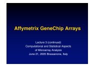
Clustered expression data for all 128
subjects, and a subset of 475 genes
showing evidence of differential
expression between groups
Slide 4

The traditional type I error rate
• The traditional p-value for a single gene:
• Define a test statistic T based on the expression data.
• Compute its value, t, for the observed data.
• Define p = P(T > t | the gene is not differentially expressed).
• Compare p to an acceptable type I (false positive) error rate.
• Suppose Chiaretti et al. had compared replicate samples, so that no gene was
differentially expressed. Comparing p-values to = .05 gives and average of
13,000 .05 = 650 false positives.
• Per-family error rate (PFER): the expected number of false positives. For the
real data, PFER 650.
Slide 5

Experiment-wide type I error rates
Not rejected Rejected Total
True null hypotheses U V m 0
False null hypotheses T S m 1
Total m – R R m 0
• Family-wise error rate: P(V > 0), i.e., the probability of one or more false
positives. For large m 0 , this is very difficult to keep small.
• False discovery rate (FDR): let Q = V/R, or 0 if R is 0. The FDR is E(Q), i.e.,
the expected fraction of false positives among all discoveries.
Slide 6

A nice property of continuous random variables
• For a continuous random
variable X, P(X = x) is 0 for any
x.
Continuous
Gaussian
Exponential
Discrete
Binomial
Geometric
• The distribution function:
Standard normal distribution function
F(x) = P(X x).
• The nice property: if we define
random U = F(X), then U is
uniformly distributed on the unit
interval [0,1].
P(X x)
0.0 0.2 0.4 0.6 0.8 1.0
-4 -2 0 2 4
x
Slide 7

A nice property of CDFs for continuous RVs
> X = rnorm(100000)
> F = pnorm
> hist(X, breaks = 50)
> hist(F(X), breaks = 50)
Histogram of X
Histogram of F(X)
Frequency
0 2000 4000 6000 8000
Frequency
0 500 1000 1500 2000
-4 -2 0 2 4
X
0.0 0.2 0.4 0.6 0.8 1.0
F(X)
Slide 8

A “nice” property?
• To compute a p-value for testing a null hypothesis H 0 , we typically…
• Define a test statistic T, and compute its value t for the observed data.
• Assume we know the distribution of T when H 0 is true: F 0 .
• Compute p = 1 – F 0 (t), i.e., define p = P(T > t | H 0 is true).
• Compare p to some .
• Now define the random variable P = 1 – F 0 (T). If H 0 is true, then…
• F 0 (T) is uniformly distribution on [0,1].
• By symmetry, P is uniformly distribution on [0,1] as well.
• Suppose 20% of genes are differentially expressed, so that
0
= m 0
m
= .80 ...
Slide 9

Observed p-values: a mixture
A.
F 0
C.
Mixture density 0 F 0 + 1 F ( 0 = 0.8)
0 10
0 10
0.0 0.2 0.4 0.6 0.8 1.0
B.
F
Density
0 0
3
II
III
I
IV
False negative
True positive
False positive
True negative
0.0 0.2 0.4 0.6 0.8 1.0
0.0 0.2 0.4 0.6 0.8 1.0
p
Slide 10

Observed p-values: a mixture
A.
F 0
C.
Mixture density 0 F 0 + 1 F ( 0 = 0.8)
0 10
0 10
0.0 0.2 0.4 0.6 0.8 1.0
B.
F
Density
0 0
3
0.0 0.2 0.4 0.6 0.8 1.0
0.0 0.2 0.4 0.6 0.8 1.0
p
Slide 11

Non-specific filtering
Slide 12

Continuing with the Chiaretti et al. ALL data
• 79 subjects with B-cell ALL:
• 37 with the BCR/ABL mutation (“Philadelphia chromosome”)
• 42 with no observed cytogenetic abnormalities
• We’ve seen that…
• Multiple testing correction becomes more extreme for larger m.
• Removal of true null hypotheses reduces the FDR associated with a particular p-
value cutoff.
• Proposal: non-specific filtering
• von Heydebreck, Huber and Gentleman, Encyclopedia of Genetics, Genomics,
Proteomics and Bioinformatics. Wiley, 2005.
• McClintick and Edenberg, BMC Bioinformatics 7:49, 2006.
Slide 13

Non-specific filtering
• For a given gene, write the data as ((c 1 ,Y 1 ),…,(c p ,Y p )).
• First group (c = 1): i = 1, …, p 1 .
• First group (c = 2): i = p 1 + 1, …, p 1 + p 2 .
• Conditions under which we expect little variation in Y:
1. Genes which are absent in both samples. (Probes will still report noise and crosshybridization,
typically at the same level in both groups.)
2. Probe sets which do not respond to target.
3. Genes which are not differentially expressed.
• A “non-specific” filter:
• Ignores c 1 , …, c p , i.e., U (I) (Y).
• Helps identify any of these three classes, based on our a priori understanding of
array behavior.
• Apply standard testing to genes passing the filter, using some U (II) (c,Y).
Slide 14

Increased rejection rate
• Stage one non-specific filter statistic: compute the overall variance
U (I) (Y) = S 2 = 1
and remove the smallest.
• Stage two: standard two-sample t-test for genes passing stage 1.
p1
p
(Y i
Y ) 2
i=1
a
b
R
0 500 1000 1500
= 0.5
= 0.4
= 0.3
= 0.2
= 0.1
= 0
R
0 500 1000 1500
0.00 0.05 0.10 0.15 0.20 0.25 0.30
FDR (BH)
0.00 0.05 0.10 0.15 0.20 0.25 0.30
qvalue
Slide 15

Increased power?
• An increased detection rate implies increased power only if we are still
controlling type I errors at the nominal level.
a
b
R
0 500 1000 1500
= 0.5
= 0.4
= 0.3
= 0.2
= 0.1
= 0
R
0 500 1000 1500
0.00 0.05 0.10 0.15 0.20 0.25 0.30
FDR (BH)
0.00 0.05 0.10 0.15 0.20 0.25 0.30
qvalue
Slide 16

Multiple testing II: impact of filtering
Slide 17

Slide 18
Notation ahead!

Conditional control
• Random variable definitions:
• V: number of false positives. FWER = P(V > 0).
• R: total number of rejections.
• Q: V / max{R, 1}. FDR = E(Q). Note that R = 0 implies that V = 0.
• M: the random set (of size M) of hypothesis passing the stage-one filter.
• U (I) and U (II) : the stage-one and stage-two test statistics.
• Conditional control is sufficient: E(Q) = E(E(Q|M)).
• Because we only reject at stage two, given M, we can assess conditional
control of type I error by considering how a procedure performs when applied
to the M conditionally distributed (U (II) I1
,…,U (II) IM
)| .
M={I1 ,…,I M
}
• Thus, FWER or FDR control is achieved if the conditional distributions of the
stage-two statistics meet requirements for the control procedure.
Slide 19

Requirements for FWER and FDR control
• Marginal properties of true-null test statistics.
• Distributions must be properly specified.
• Joint properties of all test-statistics.
• Adjustment procedures may…
…work for arbitrary dependence structure (e.g., Bonferroni and Holm).
…estimate and correct for dependence (e.g., Westfall and Young).
…require that dependence structure satisfies some assumptions.
• Assumptions about dependence structure:
• Independence!
• Subset pivotality.
• Positive regression dependence.
• Convergence of the empirical processes based on V() and R().
• Etc.
Slide 20

Independence of stage one and stage two test statistics
• For genes for which the null hypotheses is true, U (I) and U (II) are statistically
independent in both of the following cases:
• For normally distributed data:
• Stage one: overall mean, , or variance, S 2 = 1 p
Y = 1 p
p1 (Y i
Y ) 2 .
p Y
i=1 i
i=1
• Stage two: the standard two-sample t-statistic, or any location- and scaleinvariant
test statistic.
• Non-parametrically:
• Stage one: any function of the data which (i) to filter gene g only uses data
from gene g, and (ii) doesn’t depend on the order of the arguments. S 2 above,
or the IQR, are both candidates.
• Stage two: the Wilcoxon rank sum test statistic.
• Both can be extended to the multi-class context: ANOVA and Kruskal Wallis.
Slide 21

Independence: Bonferroni and Holm FWER adjustments
• Single-stage Bonferroni correction compares each p i to /m.
• The Holm step-down procedure is a more powerful variant. For ordered p-
values p (1) p (2) … p (m) , reject as long as
• Independence of U (I) and U (II) implies that the key step in proving that these
procedures control FWER still applies:
( P(V > 0) = P {U (I) > a,U (II) )
i0 i i
> b}
p (i )
<
i0
i0
P(U (I)
i
> a,U i (II) > b)
= P(U (I)
i
> a)P(P i
< )
= E(M).
m i + 1 .
Slide 22

FWER: Westfall and Young
• Westfall and Young (1993) controls FWER with more power, but depends on
the joint distribution of all p-values:
( ) .
p i
= P min
1 j m P j
p i
| H 0
C
• WY93 is valid under subset pivotality. If this holds for the one-stage
procedure, it holds for the two-stage non-specific filtering approach as well.
H 0
C
• Distribution of min P j under is typically estimated by permutation. If filtering
changes correlation structure, new structure is used by permutation!
Slide 23

FDR: Benjamini & Hochberg and Storey adjustments
• What is the FDR associated with
use of cutoff ? Naive estimator:
• V is not observable, but E(V) is
m 0 , which is bounded by m .
• E(R) cannot be computed, but
R can be used as an estimator.
FDR
() =
• Evaluating at each p (i) using m
or ˆm 0
gives BH95 or Storey
adjustments, respectively:
FDR
(p(i
)
) =
m 0
#{i : p i
}
m
#{i : p i
}
m 0
#{i : p i
p (i )
} = m 0
.
i
density
0 0
3
II I
III IV
FDR() = E
V()
R() 1 .
False negative
True positive
False positive
True negative
0.0 0.2 0.4 0.6 0.8 1.0
p
Slide 24

FDR: Benjamini & Hochberg and Storey adjustments
• The foregoing motivation for the
BH95 and Storey procedures
uses E(V()) = m 0 .
FDR() = E
V()
R() 1 .
• Marginal independence of true
null U (I) and U (II) means that this
still applies at stage two in
expectation. Define M 0 to be the
random number of true nulls
passing stage 1. Then
E(V()) = P(U (I) i
> a, P
i i
< )
0
= P(U (I) i
> a)P( P
i i
< )
0
= E(M 0
).
density
0 0
3
II I
III IV
False negative
True positive
False positive
True negative
0.0 0.2 0.4 0.6 0.8 1.0
p
Slide 25

Counterexamples
Slide 26

Counterexample #1: normality matters
• Filter on S 2 , test using T.
• For true null hypotheses, data
are i.i.d. normal with probability
p, but heavily skewed with
probability 1 – p. Let latent X
indicate mixture component
identity.
Frequency
0 100 200 300 400
^ | X = 0
0.0 0.5 1.0 1.5 2.0 2.5 3.0
^ | X = 1
Frequency
0 50 100 150 200 250
T(Y) | X = 0
4 2 0 2 4
T(Y) | X = 1
• The filter statistic is now
predictive for X.
• The conditional distribution of T
will be more weighted towards
the X = 1 case than the
unconditional distribution.
Frequency
0 100 200 300 400
0.0 0.5 1.0 1.5 2.0 2.5 3.0
Frequency
0 50 100 150 200 250
4 2 0 2 4
Slide 27

Counterexample #2: the limma t-statistic
• Filter on S 2 , test using the limma
moderated t-statistic.
• The moderated t-statistic is not
scale invariant, due to the effect
of the global variance estimator.
• This is more pronounced for
small n — precisely the context
in which limma is most useful.
• Filtering on overall mean rather
than variance “solves” the
problem.
|t|
0.0 0.5 1.0 1.5 2.0 2.5 3.0 3.5
Moderated t and overall variance
0.5 1.0 1.5 2.0
S
Slide 28

Counterexample #2: the limma t-statistic
Unconditional pvalues
Conditional pvalues
Frequency
0 10 20 30 40 50 60
Frequency
0 10 20 30 40 50
0.0 0.2 0.4 0.6 0.8 1.0
fit$p.value[, 2]
0.0 0.2 0.4 0.6 0.8 1.0
fit$p.value[S > median(S), 2]
Slide 29

Conclusions
• In actual examples, use of an independent filter leads to (biologically)
significant increases in the number of genes identified.
• Some commonly used stage one/stage two test statistic pairs are statistically
independent for genes which are not differentially expressed…
• …but others are not! The non-specific criterion is not enough.
• Given this independence, Bonferroni and Holm FWER control is valid in the
two-stage procedure. Likewise for FDR-controlling procedures which make no
assumptions about independence.
• Correlation structure may change under filtering. Permutation-based Westfall
and Young correction accounts for this. FDR control could theoretically suffer,
although the practical impact is likely to be small.
• Effect of filtering on correlation can also be checked, and impact, assessed.
Slide 30