ON GLOBAL RIEMANN-CARTAN GEOMETRY

ON GLOBAL RIEMANN-CARTAN GEOMETRY
Prof. Sergey E. Stepanov
Finance University
under the
Government of Russian Federation
Moscow (Russia)
E-mail: s.e.stepanov@mail.ru
1

1. History of the Metrically-Affine Theory
The beginning of metrically-affine space (manifold) theory was marked by E. Cartan in 1923-1925, who suggested
using an asymmetric linear connection ∇ having the metric property ∇ g = 0
theory of gravity (ECT).
. His theory was called Einstein-Cartan
[1] Cartan Е. Sur les variétés à connexion affine et la théorie de la relativité généralisée. Part I, Ann. Ec. Norm., 40
(1923), 325-412.
[2] Cartan Е. Sur les variétés à connexion affine et la théorie de la relativité généralisée. Part I, Ann. Ec. Norm., 41
(1924), 1-25.
[3] Cartan Е. Sur les variétés à connexion affine et la théorie de la relativité généralisée. Part II, Ann. Ec. Norm., 42
(1925), 17-88.
[4] Cartan E. On manifolds with an affine connection and the theory of general relativity. Napoli: Bibliopolis, 1986, 199
p.
[5] Trautman A. The Einstein-Cartan theory. Encyclopedia of Mathematical Physics: Edited by Fracoise J.-P., Naber
G.L., Tsou S.T. – Oxford: Elsevier, 2 (2006), 189-195.
2

T. Kibble and D. Sciama have found a connection between the torsion S of the connection ∇ and the spin tensor s
of matter. Subsequently, other physical applications of ECT were found.
[6] Kibble T.W.B. Lorenz invariance and the gravitational field. J. Math. Phys, 2 (1961), 212-221.
[7] Sciama D.W. On the analogy between change and spin in general relativity. Recent developments in General
Relativity. – Oxford: Pergamon Press & Warszawa: PWN, 1962, pp. 415-439.
[8] Penrose R. Spinors and torsion in General Relativity. Found. of Phys 13 (1983), 325-339.
[9] Ruggiero M.L., Tartaglia A. Einstein-Cartan theory as a theory of defects in space-time. Amer. J. Phys. 71 (2003),
1303-1313.
The Einstein-Cartan theory was generalized by omitting the metric property of the linear connection ∇, i.e. the
nonmetricity tensor Q = ∇g
≠ 0 . The new theory was called the metrically-affine gauge theory of gravity (MAG).
[10] Hehl F.W., Heyde P. On a New Metric-Affine Theory of Gravitation. Physics Letters B. 63: 4 (1976), 446-448.
3

The E. Cartan idea was reflected in the well-known books in differential geometry of the first half of the last century.
Now there are hundreds works published in the frameworks of ECT and MAG, and moreover, the published results
are of applied physical character.
[11] Schouten J.A., Struik D.J. Einführung in die neuere methoden der differntialgeometrie, I. Noordhoff: Groningen-
Batavia, 1935.
[12] Schouten J.A., Struik D.J. Einführung in die neuere methoden der differntialgeometrie, II. Noordhoff: Groningen-
Batavia, 1938.
[13] Eisenhart L.P. Non Riemannian geometry. New York: Amer. Math. Soc. Coll. Publ., 1927.
[14] Eisenhart L.P. Continuous groups of transformations. Prinseton: Prinseton Univ. Press, 1933.
[15] Puetzfeld D. Prospects of non-Riemannian cosmology. Proceeding of the of 22 nd Texas Symposium on
Relativistic Astrophysics at Stanford University (Dec. 13-17, 2004). California: Stanford Univ. Press, 2004, 1-5.
[16] Hehl F.W., Heyde P., Kerlick G.D., Nester J.M. General Relativity with spin and torsion: Foundations and
prospects. Rev. Mod. Phys, 48: 3 (1976), 393-416.
4

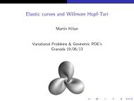
Classification of known kinds of metrically-affine spaces (manifolds) is presented in the following diagram.
Metric-affine
Metric-affine
manifolds
manifolds
Q = n -1 tr Q g
Weyl-Cartan
Weyl-Cartan
= 0 manifolds
manifolds
Q = 0
Weyl
Weyl
manifolds
manifolds
Q = 0
= 0 Q = 0
Riemannian
Riemannian
manifolds
manifolds
= 0
Flat
Flat
manifolds
manifolds
Riemannian
Riemannian
–
–
Cartan
Cartan
manifolds
manifolds
manifolds
manifolds
= 0 = 0
= 0
Weitzenböck
Weitzenböck
manifolds
manifolds
5

For long time, among all forms metrically-affine space, only quarter-symmetric metric spaces and the semisymmetric
metric spaces were considered in differential geometry.
[17] Yano K. On semi-symmetric metric connection. Rev. Roum. Math. Pure Appl., 15 (1970), 1579-1586.
[18] Nakao Z. Submanifolds of a Riemannian manifold semi-symmetric metric connections. Proc. Amer. Math. Soc.,
54 (1976), P. 261-266.
[19] Barua B., Ray A.K. Some properties of semi-symmetric connection in Riemannian manifold. Ind. J. Pure Appl.
Math., 16 (1985), No. 7, 726-740.
[20] Chaubey S.K., Ojha R.H. On semi-symmetric non-metric and quarter symmetric metric connections. Tensor,
N.S., 70 (2008), 202-213.
[21] Segupta J., De U.C., Binh T.Q. On a type of semi-symmetric connection on a Riemannian manifold. Ind. J. Pure
Appl. Math., 31: 12 (2000), 1650-1670.
[22] Muniraja G. Manifolds admitting a semi-symmetric metric connection and a generalization of Shur’s theorem. Int.
J. Contemp. Math. Sciences, 3: 25 (2008), 1223-1232.
6

The development of geometry of metrically-affine spaces “in the large” was stopped at the results of K. Yano, S.
Bochner and S. Goldberg obtained in the middle of the last century. In their works, in the frameworks of RCT, they
proved “vanishing theorems” for pseudo-Killing and pseudo-harmonic vector fields and tensors on compact Riemann-
Cartan manifolds with positive-definite metric tensor g and the torsion tensor S such that trace S = 0.
Y. Kubo, N. Rani and N. Prakash have generalized their results by introducing in consideration compact Riemann-
Cartan manifolds with boundary.
[23] Bochner S., Yano K. Tensor-fields in non-symmetric connections. The Annals of Mathematics, 2 nd Ser. 56: 3
(1952), 504-519.
[24] Yano K., Bochner S. Curvature and Betti number. Princeton: Princeton University Press, 1953.
[25] Goldberg S.I. On pseudo-harmonic and pseudo-Killing vector in metric manifolds with torsion. The Annals of
Mathematics, 2 nd Ser. 64: 2 (1956), 364-373.
[26] Kubo Y. Vector fields in a metric manifold with torsion and boundary. Kodai Math. Sem. Rep. 24 (1972), 383-395.
[27] Rani N., Prakash N. Non-existence of pseudo-harmonic and pseudo-Killing vector and tensor fields in compact
orientable generalized Riemannian space (metric manifold with torsion) with boundary. Proc. Natl. Inst. Sci. India.
32: 1 (1966), 23-33.
7

2. Riemann-Cartan manifolds
A Riemann-Cartan manifold is a triple ( M ,g,∇)
, where ( M ,g ) is a Riemannian n-dimensional ( n ≥ 2)
manifold with
linear connection ∇ having nonzero torsion S such that ∇g = 0 .
[1] Trautman A. The Einstein-Cartan theory. Encyclopedia of Mathematical Physics: Edited by Fracoise J.-P., Naber
G.L., Tsou S.T. – Oxford: Elsevier, 2 (2006), 189-195.
The deformation tensor T defined by the identity
following properties
(i)
T is uniquely defined;
(ii) S ( X, Y ) ( T ( X,
Y ) −T
( Y,
X ))
;
(iii)
= 2
1
g ( T ( X ,Y ),Z
) + g ( T ( X ,Z ),
Y ) = 0
2
T ∈C
∞ TM ⊗Λ M since ∇ = 0 ⇔ g ;
(iV) g ( T ( Y ,Z ),
X ) g ( S( X ,Y ),Z
) + g ( S( X ,Z ),Y
) + g( S( Y ,Z ),
X )
(V) trace T = 2 trace S .
= ;
Т := ∇ −∇
where ∇ is the Levi-Civita connection on (M, g) has the
[2] Yano K., Bochner S. Curvature and Betti number. Princeton: Princeton University Press, 1953.
8
3. Cappozziello-Lambiase-Stornaiolo classification of Riemann-Cartan manifolds

We know that
S
b
∈C
∞ Λ
2 M ⊗TM
( M ) ⊕ Ω ( M ) ⊕ ( M )
∗
M ⊗ T M ≅ Ω
2
3
Λ 2 Ω
1
. In turn, the following pointwise O(q)-irreducible decomposition holds
. Here, q = g(x) for an arbitrary point x ∈ M
projections on the components of this decomposition are defined by the following relations:
(1)
S
b
( )
b
b
b
( X , Y,
Z ) = −1 S ( X,
Y,
Z ) + S ( Y,
Z,
X ) + S ( Z,
X,
Y )
3 ;
( X,
Y,
Z ) g( Y,
Z ) θ ( X ) g( X,
Z ) θ( Y )
(2) S b
−
(3)
S
b
= ;
( )
b
(1) b
(2) b
( X , Y,
Z ) S ( X,
Y,
Z ) − S ( X,
Y,
Z ) − S ( Z,
X,
Y )
= ,
b
where S ( X,
Y,
Z ) = g( S( X,
Y ),
Z ) and := ( n −1) −1 trace S
θ .
. In this case, the orthogonal
[1] Bourguignon J.P. Formules de Weitzenbök en dimension 4. Géométrie Riemannienne en dimension 4: Seminaire
Arthur Besse 1978/79. – Paris: Cedic-Fernand Nathan, 1981.
We say that a Riemann-Cartan manifold ( M ,g,∇)
belongs to the class Ω
α or
the tensor field
b
S is a section of corresponding tensor bundle α
( Ě )
Ω or ( Ě ) ⊕ Ω ( Ě )
Ωα
⊕ Ω
β for α , β = 1 , 2,
3 and α < β if
Ω .
α
β
[2] Capozziello S., Lambiase G., Stornaiolo C. Geometric classification of the torsion tensor in space-time. Annalen
Phys., 10 (2001), 713-727.
9

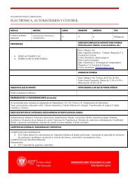
All these classes of Riemann-Cartan manifolds are presented in the following diagram.
Riemannian
Riemannian
-
-
-
-
Cartan
Cartan
manifolds
manifolds
Ω 1 ⊕
Ω
1 ⊕ 2 2
Ω 1
Ω 2
Ω 1
Ω 1 ⊕
Ω
1 ⊕ 3
Ω 2
3
Ω 2 ⊕
Ω
2 ⊕ 3
Ω
3
3 3
Riemannian
Riemannian
manifolds
manifolds
10

4. The class Ω 1 ⊕ Ω 2 of Cappozziello-Lambiase-Stornaiolo classification
Lemma 4.1. A Riemann-Cartan manifold ( ,∇)
satisfies an algebraic equation of the form
b
of Riemann-Cartan manifolds
M,g belongs to the class Ω1 ⊕ Ω
2 if and only if its torsion tensor
b
( X,
Y,
Z ) + S ( X,
Z,
Y ) = g( X,
Z ) B( Y ) + g( X,
Y ) B( Z ) + g( Y Z ) A( X )
S ,
for some smooth A, B ∈ С
∞ Т
∗ М and arbitrary vector fields X, Y, Z ∈С ∞ ТМ
Lemma 4.2. The class Ω 2 of Riemann-Cartan manifolds ( M,g ,∇)
consists of semisymmetric Riemannian-Cartan
manifolds.
Lemma 4.3. A Riemann-Cartan manifold ( M,g ,∇)
belongs to the class Ω 1 if and only if its torsion tensor satisfies the
property
S
b
∈C
∞ Λ
3
M
. In particular, this class includes spaces of semisimple groups.
[1] Eisenhart L.P. Continuous groups of transformations. Princeton: Princeton Univ. Press, 1933.
[2] Yano K., Bochner S. Curvature and Betti number. Princeton: Princeton University Press, 1953.
[3] Fabri L. On a completely antisymmetric Cartan torsion tensor. Annalen de la Foundation de Broglie 32: 2-3 (2007),
215-228..
11

We know that
5. Vanhecke-Tricerri classification of Riemann-Cartan manifolds
Ň
b
∈ŇĚ
⊗C
∞
2
Λ M
. In turn, the following pointwise O(q)-irreducible decomposition holds
T*M ⊗ Λ 2 M ≅ Ψ 1 (M) ⊕ Ψ 2 (M) ⊕ Ψ 3 (M). In this case, the orthogonal projections on the components of this
decomposition are defined by the following relations:
(1)
Т
Т
b
( )
1 b
b
b
( X ,Y ,Z ) 3 Т ( X ,Y ,Z ) + Т ( Y ,Z, X ) + Т ( Z, X ,Y )
= − ;
( X ,Y ,Z ) = g( X ,Z ) ω( Y ) − g( X ,Y ) ω( Z )
(2) b
;
(3)
Т
b
( )
b
(1) b
(2) b
( X ,Y ,Z ) Т ( X ,Y ,Z ) − Т ( Y ,Z, X ) − Т ( Z, X ,Y )
= ,
b
−1
where Т ( X,
Y,
Z ) = g( T ( X,
Y ),
Z ) and : = ( n −1) trace Т
ω .
[1] Bourguignon J.P. Formules de Weitzenbök en dimension 4. Géométrie Riemannienne en dimension 4: Seminaire
Arthur Besse 1978/79. Paris: Cedic-Fernand Nathan, 1981.
We say that a Riemann-Cartan manifold ( M ,g,∇)
belongs to the class Ψ α or
b
tensor field Т is a section of corresponding tensor bundle Ψ α ( М ) or α ( М ) ⊕Ψβ
( М )
Ψ ⊕Ψ
for , β = 1 , 2,
3
α
Ψ .
β
α and α < β if the
[2] Tricerri F., Vanhecke L. Homogeneous structures. Progress in mathematics (Differential geometry), 32 (1983),
234-246.
The spaces
12
∗
Λ 2 М ⊗Т
М and Т М ⊗Λ М
∗
2
, as well as their irreducible components, are isomorphic. Therefore these
two classifications are equivalent. Moreover, corresponding classes of Riemann-Cartan manifolds from these two
classifications coincide.

6. Examples of Riemann-Cartan manifolds
Consider a Euclidian sphere S 2 = {S 2 \ north pole} of radius R excluding the north pole and with the standard
Riemannian metric g 11 = R 2 cos 2 ϕ, g 22 = R 2 , g 12 = g 21 = 0 where
1 2
х =ϑ , х = ϕ for denote the standard spherical
coordinates of S 2 . Then X 1 = {(R cos ϕ) -1 , 0}, X 2 = {0, R -1 } are vectors of standard orthogonal basis of all vector fields
on S 2 .
There is a non-symmetric metric connection ∇ with coefficients
1
Γ - tanϕ
and other Γ α β = γ 0 such that ∇ = 0
where α , β,
γ =1,
2.
For this connection ∇ the curvature tensor R = 0 and the torsion tensor S has components
( ) 1 tanϕ
1
12 = 2 −
2
12 =
S , 0
21 =
Х Х α β
S . Therefore, S 2 with g and ∇ is an example of a Riemann-Cartan manifold manifold ( g,∇)
In addition if R = 0 then ∇ has name Weitzenböck or a teleparallel connection.
M, .
[1] Cartan Е. Sur les variétés à connexion affine et la théorie de la relativité généralisée. Part I, Ann. Ec. Norm., 41
(1924), 1-25.
[2] Aldrovandi R., Pereira J. G., and Vu K. H. Selected topics in teleparallel gravity. Вrazilian Journal of Physics, 34:
4A (2004), 1374-1380.
[3] Wu Y.L., Lee X.J. Five-dimensional Kaluza-Klein theory in Weizenböck space. Phys. Letters A, 165 (1992), 303-
306.
13

A homogeneous Riemannian manifold (M, g) is the connected Riemannian manifold (M, g) whose isometry group is
transitive.
By the Tricerri and Vanhecke theorem, a complete connected Riemannian manifold (M, g) is
2
homogeneous iff a tensor field T ∈С
∞ ТМ ⊗Λ М such that = 0
∇R and = 0
∇T for the connection = ∇ + T
∇ .
In this case, ∇g = 0 and, therefore, a homogeneous Riemannian manifold is an example of the Riemannian-Cartan
manifold( M, g,∇)
.
[4] Tricerri F., Vanhecke L. Homogeneous structures on Riemannian manifolds. London Math. Soc.: Lecture Note
Series., Vol. 83. Cambridge University Press, London, 1983.
An almost Hermitian manifold is defined as the triple (M, g, J), where the pair (M, g) is a Riemannian 2m-dimensional
manifold with almost complex structure J
[5] Kobayshi S., Nomizu K. Foundations of Riemannian geometry, Vol. 2. Interscience publishers, New York-London,
1969.
∗
∈ ТМ ⊗Т
М compatible with the metric g, i.e. J 2 −Id
TM
= and g ( J, J) = g . In
this case, ∇g = 0 for the connection∇
=∇+∇J
, and, therefore, an almost Hermitian manifold (M, g, J), together with
the connection
,
∇ =∇+∇J
, is an example of the Riemannian-Cartan manifold (M, g,∇).
14

The classification of almost Hermitian manifolds is well known, it is based on the pointwise U(m)-irreducible
decomposition of the tensor
∇ Ω, where Ω (X, Y) = g(X, JY).
Almost semi-Kählerian manifolds are isolated by the condition trace ∇ J = 0 and are an example of Riemann-
Cartan manifolds of class Ω 1 ⊕ Ω 2 .
Almost Kählerian manifolds are isolated by the condition dΩ = 0 and are an example of Riemann-Cartan manifolds
of class Ω 2 ⊕ Ω 3 .
Nearly Kählerian manifolds are isolated by the condition dΩ = 3 ∇Ω and are an example of Riemann-Cartan
manifolds of class Ω
1 .
[6] Gray A., Hervella L. The sixteen class of almost Hermitean manifolds. Ann. Math. Pura Appl., 123 (1980), 35-58.
15

7. Weitzenböck manifolds
A Riemann-Cartan manifold ( M ,g,∇)
is called the Weitzenböck or teleparallel manifold if the curvature tensor R of
the nonsymmetric metric-affine connection ∇ vanishes.
[1] Hayashi K., Shirafuji T. New general relativity. Phys. Rev. D, 19 (1979), 3524-3553.
[2] Wu Y.L., Lee X.J. Five-dimensional Kaluza-Klein theory in Weizenböck space. Phys. Letters A, 165 (1992), 303-
306.
[3] Aldrovandi R., Pereira J.G., Vu K.H. Selected topics in teleparallel gravity. Brazilian J. Ph., 34 (2004), 1374-1380.
Lemma 7.1. If the Weitzenböck manifold ( M ,g,∇)
with positive-definite metric g belongs to the class Ω 1 then
n
( X,X ) T ( X,e ,e ) T ( X,e , e ) ≥ 0
Ric = ∑ i j
i j for Ricci tensor Ric of the Riemannian manifold (M, g) and an arbitrary orthonormal
i,j = 1
basis {e 1 , e 2 , … , e n }.
Lemma 7.2. If the Weitzenböck manifold ( M ,g,∇)
belongs to the class Ω 2 then the Weyl tensor W of the
Riemannian manifold (M, g) vanishes and (M, g) for n ≥ 4 is a conformally flat.
Lemma 7.3. If the Weitzenböck manifold ( M ,g,∇)
belongs to the class Ω 3 then s = – 2
2
S ≤ 0 for the scalar
curvature s of the Riemannian manifold (M, g).
16

8. Green theorem for a Riemann-Cartan manifold
∫
=
Let (M, g) be a compact oriented Riemannian manifold then the classical Green’s theorem ( div X ) dV
0 has the
∫
=
form ( trace∇X
) d V 0 for an arbitrary smooth vector field X and the volume element dV.
М
М
[1] Yano K., Bochner S. Curvature and Betti number. Princeton: Princeton University Press, 1953.
Since the dependence
∇ = ∇ + Т holds on ( ,g,∇)
M , it follows that trace ∇ X = trace∇X
+2( trace S)X
. Whence, by the
Green’s theorem, we deduce the Green’s theorem ( trace ∇X
−2( traceS ) X ) d V 0 for a Riemann-Cartan manifold
( M ,g,∇)
.
∫ =
M
Goldberg S., Yano K. and Bochner S. and also Kubo Y., Rani N, and Prakash N. proved their “vanishing theorems”
on compact oriented Riemann-Cartan manifolds under the condition that
∫
trace V = 0
theorem has the form ( ∇X
)
М
div X = trace∇X
. In this case Green’s
d . These Riemann-Cartan manifolds belong to the class Ω 1 ⊕ Ω 3 .
17

[2] Bochner S., Yano K. Tensor-fields in non-symmetric connections. The Annals of Mathematics, 2 nd Ser. 56(1952),
No. 3, 504-519.
[3] Yano K., Bochner S. Curvature and Betti number. Princeton: Princeton University Press, 1953.
[4] Goldberg S.I. On pseudo-harmonic and pseudo-Killing vector in metric manifolds with torsion. The Annals of
Mathematics, 2 nd Ser. 64 (1956), No. 2, 364-373.
[5] Kubo Y. Vector fields in a metric manifold with torsion and boundary. Kodai Math. Sem. Rep. 24 (1972), 383-395.
[6] Rani N., Prakash N. Non-existence of pseudo-harmonic and pseudo-Killing vector and tensor fields in compact
orientable generalized Riemannian space (metric manifold with torsion) with boundary. Proc. Natl. Inst. Sci. India.
32 (1966), No. 1, 23-33.
18

9. Scalar and complete scalar curvature
of Riemann-Cartan manifolds
It is well known that the curvature tensor R of the linear non-symmetric connection ∇ of a Riemann-Cartan
manifold ( ,g,∇)
2
2
M is a section of the tensor bundle Λ M ⊗ Λ M . Therefore the scalar curvature of the Riemann-
Cartan manifold ( ,g,∇)
a Riemannian manifold (M, g).
n
M we can define by the formula s ∑ R( e ,e ,e ,e )
_
= as an analogy to the scalar curvature s of
The dependence between the scalar curvatures s and s is described in the following formula
i = 1
( 1) b
2
( ) ( 2 ) b
2 ( 3 ) b
2
b
= s − S −2
n −2
S + 2 S − div ( trace S ). (9.1)
s 4
In particular, for the Weitzenböck connection ∇ we have the identity s = 0. Then the formula (9.1) can be rewritten in
the following form
( 1) b
2
( ) ( 2 ) b
2 ( 3 ) b
2
b
S + 2 n −2
S −2
S 4div ( traceS )
s = +
.
i
j
i
j
[1] Yano K., Bochner S. Curvature and Betti number. Princeton: Princeton University Press, 1953.
[2] Stepanov S.E., Gordeeva I.A. Pseudo-Killing and pseudo harmonic vector field on a Riemann-Cartan manifold.
Mathematical Notes, 87: 2 (2010), 238-247.
19

We consider a Riemann-Cartan manifold ( M ,g,∇)
of the class Ω 1 which is characterized by the conditions
( 2 ) ( 3
=
)
S = 0
S that is equal to S
b 3
∈C
∞ Λ M . For this condition the identity (9.1) can be rewritten as s = s −
( 1) S
2
. Hence
we have
s ≤ s , and equality is possible only if ∇ = ∇. The following theorem holds.
Theorem 9.1. The scalar curvatures s and s of the metric connection ∇ and of the Levi-Civita connection ∇ of an
n-dimensional Riemannian-Cartan manifold ( M,g ,∇)
of the class Ω 1 satisfy the inequality s ≤ s . The equality s = s is
possible only if
∇ = ∇.
Let ( M ,g,∇)
be a compact Riemann-Cartan manifold, we define its complete scalar curvature as the number
s ( M ) =
∫
s d V as an analogue of the complete scalar curvature s( M ) = ∫ s d V
M
of a Riemannian manifold.
M
The dependence between the complete scalar curvatures s(M) and s (M) is described in the following formula
∫
( )
( 1) b
2
( ) ( ) ( ) ( 2
= − + −
) b
2
−
( 3 ) b
2
s M s M S 2 ň 2 S 2 S dV . (9.2)
In particular, for the Weitzenböck connection ∇ we have the integral identity
M
∫
b
2
( S )
( 1) b
2
( ) ( ) ( 2
= + −
) b
2
−
( 3
M S 2 ň 2 S 2
)
s dV .
M
20

For a compact Riemann-Cartan manifold ( M ,g,∇)
of the class Ω 1 ⊕ Ω 2 , we have
Then the following theorem is true.
s
⎛
⎝
( ) ( )
( 1) b
M = s M −∫
⎜ S + ( n − ) ( 2
2 2
)
M
2
S
b
2
⎞
⎟dV
⎠
. (9.3)
Theorem 9.2. The complete scalar curvatures s ( M ) and s ( M ) of Riemannian compact oriented manifold ( M ,g ) and
a compact oriented Riemann-Cartan manifold ( M,g ,∇)
of class Ω 1 ⊕ Ω 2 are related by the inequality ( M ) s( M )
s ≤ .
For dimM
≥3
, the equality is possible if the connection ∇ coincides with the Levi-Civita connection ∇ of the metric
g, for n = 2, if ∇is a semi-symmetric connection.
For a compact Weitzenböck manifold ( M,g ,∇)
of the class Ω 1 ⊕ Ω 2 the inequality ( M ) ≥ 0
formulate (see Lemma 7.1)
s holds. Therefore we can
Corollary 1. There are not Weitzenböck connections ∇ of the class Ω 1 ⊕ Ω 2 on a compact Riemannian manifold
with ( M ) < 0
s .
21

Knowing the definition of the scalar curvatures s and s and taking account of the positive definiteness of the metric g,
we can prove the following corollary.
Corollary 2. On compact oriented Riemannian manifold (M, g) with negative-semidefinite (resp. negative-definite) the
scalar curvature s, there is no non-symmetric metric connection ∇ of class Ω 1 ⊕ Ω 2 with positive-definite (resp.
−
−
positive-semi definite) quadratic form (X, X) for the Ricci tensor
Ric Ric
For a Riemann-Cartan manifold ( ,g,∇)
theorem is true.
of the connection ∇ and any vector field X.
( 3 ) b
2
M of the class Ω 3 , we have s ( M ) = s( M ) + 2∫
S dV . Then the following
M
Theorem 9.3. The complete scalar curvatures s(M) and s ( M ) of Riemannian manifold ( M ,g ) and a Riemann-Cartan
manifold ( M,g ,∇)
of class Ω 3 a related by the inequality ( M ) s( M )
coincides with the Levi-Civita connection ∇ of the metric g.
s ≥ . The equality is possible if the connection ∇
Knowing the definition of the scalar curvatures s and s we can prove the following corollary.
Corollary 4. On Riemannian manifold (M, g) with positive-semidefinite (resp. positive-definite) the scalar curvature s,
there is no non-symmetric metric connection ∇ of class Ω 3 with negative-definite (resp. negative-semi definite)
−
−
quadratic form (X, X) for the Ricci tensor
Ric Ric
22
of the connection ∇ and any smooth vector field X.

The differential equation ( ∇ ξ,Y
) + g ( X ∇ ξ ) = 0
manifold ( ,g,∇)
10. Pseudo – Killing vector fields
g defining the pseudo-Killing vector field on a Riemann-Cartan
X ,
Y
( )
b
b
M can be represented in the equivalent form ( L g )( X,
Y ) = 2 S ( ξ,
X,
Y ) S ( ξ,
Y,
X ) where L ξ is
the Lie derivative with respect to ξ.
ξ +
[1] Goldberg S.I. On pseudo-harmonic and pseudo-Killing vector in metric manifolds with torsion. The Annals of
Mathematics, 2 nd Ser. 64: 2 (1956), 364-373.
Let ( M ,g,∇)
belong to the class Ω 1 ⊕ Ω 2 then ( Lξ
g )( X ,Y ) = ( 2g
( X ,Y ) θ ( ξ ) − g ( X , ξ ) θ ( Y ) − g ( ξ,
Y ) θ ( ξ ) )
2 and hence
( Lξ
g )( X ,Y ) = 4g
( X , Y ) θ( ξ )
⊥
for arbitrary smooth vector fields X and Y belong to the hyperdistribution ξ orthogonal to ξ.
Moreover, the second fundamental form
⊥ ⊥
Q of ξ has the form
⊥
Q = 4 g ⊗ξ
.
Theorem 10.1. A pseudo-Killing (non-isotropic) vector field ξ on a Riemann-Cartan manifold ( M ,g,∇)
of class Ω 1 ⊕
⊥
Ω 2 is an infinitesimal (n – 1)-conformal transformation and the hyperdistribution ξ orthogonal to ξ is umbilical.
[2] Tanno S. Partially conformal transformations with respect to (m – 1)-dimensional distributions of m-dimensional
Riemannian manifolds. Tôhoku Math. J., 17: 17 (1965), 358-409.
[3] Reinhart B.L. Differential geometry of foliations. Berlin-New York: Springer-Verlag, 1983.
23

On a compact oriented manifold (M, g) with globally defined umbilical hyperdistribution, the following integral formula
holds
∫ ⎜
⎛ ⊥
2
⊥
2
( , ς) − F −( n −1
)( n −2)
H ⎟
⎞
dv =
M
r 0
⎝
⎠
where ς is the unit vector field orthogonal to this hyperdistribution and
ς (10.3)
hyperdistribution. Then from this formula, we deduce that the following theorem is true.
⊥
Н is a mean curvature vector of this
Theorem 10.2. Let a compact oriented n-dimensional (n > 2) Riemann-Cartan manifold ( M ,g,∇)
with positive-definite
metric tensor g belong to the class Ω 1 ⊕ Ω 2 . If the condition Ric( ξ, ξ) ≤ 0 holds for a pseudo-Killing vector field ξ then
the hyperdistribution
⊥
ξ is integrable with maximal totally geodesic manifolds and the metric form of the manifold has
n
the following form in a local coordinate system x 1 ,..., x of a certain chart (U, ψ )
ds
= g
ab
1 n −1
a b
1 n n n
( x ,..., x ) dx ⊗ dx + g ( x ,..., x ) dx ⊗ dx
2 for a,b
=1,...,n
−1
.
nn
[3] Stepanov S.E. An integral formula for a Riemannian almost-product manifold. Tensor, N.S., 55: 3 (1994), 209-213.
[4] Stepanov S.E., Gordeeva I.A. Pseudo-Killing and pseudo harmonic vector field on a Riemann-Cartan manifold.
Mathematical Notes, 87: 2 (2010), 238-247.
24

11. Vanishing theorems for pseudo-Killing vector fields
The analysis of the integral formula (10.3) allows to draw a conclusion that the following theorem is true.
Theorem 11.1. Let a compact oriented n-dimensional (n > 2) Riemann-Cartan manifold ( M ,g,∇)
with positivedefinite
metric tensor g belong to the class Ω 1 ⊕ Ω 2 . If the Ricci tensor Ric of the Levi-Civita connection ∇ of the
metric g is negative, then on ( M ,g,∇)
there are no nonzero pseudo-Killing vector fields.
The Laplacian of the length function F = ½ g (ξ , ξ ) of a pseudo-Killing vector field on a Riemann-Cartan manifold
(M, g,∇) is found from the relation
n
∑
∆F
= g
___
n
( ∇ , ∇ξ
) −Ric( ξ,
ξ ) + 2∑ g( S( ξ,
ei
),
∇e i
ξ )
2
for ∆F = ( ∇ F )( ei , e i
) and a local orthonormal basis { e 1 , … , e n }.
i=
1
ξ (11.1)
i=
1
[1] Stepanov S.E., Gordeeva I.A. On existence of pseudo-Killing and pseudo-harmonic vector fields on Riemannian-
Cartan manifolds. Zb. Pr. Inst. Mat. NaN Ukr. 6: 2 (2009), 207-222.
25

Using the formula (11.1) we can prove the following theorems.
Theorem 11.2. Let a Riemann-Cartan manifold ( M ,g,∇)
with positive-definite metric tensor g belong to the class
Ω 2 . If the length function F = ½ g (ξ , ξ ) of a pseudo-Killing vector field ξ has a local maximum at a point x ∈ M
of the manifold at which the quadratic form Ric ____
(X, X) is negative-definite, then ξ vanishes at this point and in a
certain its neighborhood.
Theorem 11.3. Let a Riemann-Cartan manifold ( M ,g,∇)
with positive-definite metric tensor g belong to the class
Ω 3 . If the length function F = ½ g (ξ , ξ ) of a pseudo-Killing vector field ξ has a local maximum at a point x ∈ M
at which the quadratic form Ric ____
(X, X) is negative-definite, then ξ vanishes on the whole manifold.
[2] Stepanov S.E., Gordeeva I.A., Pan’zhenskii V.I. Riemann-Cartan manifolds. Journal of Mathematical Science
(New York), 169: 3 (2010), 342-361.
26

12. Pseudo-harmonic vector fields
A vector field ξ on a Riemann-Cartan manifold ( M ,g,∇)
with positive-definite metric tensor g is said to be
pseudo -harmonic if it is a solution of the system of differential equations g ( ∇ ,Y ) − g ( X, ∇ ξ ) 0
0.
[1] Goldberg S.I. On pseudo-harmonic and pseudo-Killing vector in metric manifolds with torsion. The Annals of
Mathematics, 2 nd Ser. 64: 2 (1956), 364-373.
Theorem 12.1. Let a compact oriented n-dimensional (n > 2) Riemann-Cartan manifold ( M ,g,∇)
with positivedefinite
metric tensor g belong to the class Ω 1 ⊕ Ω 2 . If the condition Ric ( ξ , ξ) ≥0
holds for a pseudo-harmonic
⊥
vector field ξ then the hyperdistribution ξ orthogonal to ξ is umbilical.
−−−
ξ ; trace ∇ ξ =
X Y
=
Theorem 12.2. Let a compact oriented n-dimensional (n > 2) Riemann-Cartan manifold ( M ,g,∇)
with positive-
___
definite metric tensor g belongs to the class Ω 2 . If the condition Ric ( ξ, ξ) ≥0
holds for a pseudo-harmonic vector
⊥
field ξ then the hyperdistribution ξ is integrable with maximal totally umbilical manifolds and the metric form of
n
the manifold has the following form in a local coordinate system x 1 ,..., x of a certain chart (U, ψ )
ds
2
= σ
1 n 1 n−1
a b
1 n n n
( x ,...,x ) g ( x ,...,x ) dx ⊗ dx + g ( x ,...,x ) dx ⊗ dx
ab
nn
for a,b
=1,...,n
−1.
27

The Laplacian of the length function F = ½ g (ξ , ξ ) of a pseudo-harmonic vector field on a Riemann-Cartan
manifold (M, g,∇) of the class Ω 1 ⊕ Ω 2 has the form
∆F
= g
2
n − 2
___
( ∇ , ∇ξ
) + Ric( ξ,
ξ ) + g( ∇F,
traceS )
ξ (12.1)
Using the formula (12.1) we can prove the following theorem.
Theorem 12.2. Let a Riemann-Cartan manifold ( M ,g,∇)
with positive-definite metric tensor g belong to the class
Ω 1 ⊕Ω 2 . If the length function F = ½ g (ξ , ξ ) of a pseudo-harmonic vector field ξ has a local maximum at a
point x ∈ M at which the quadratic form Ric ____
(X, X) is positive-definite, then ξ vanishes at this point and in a
certain its neighborhood.
[2] Stepanov S.E., Gordeeva I.A., Pan’zhenskii V.I. Riemann-Cartan manifolds. Journal of Mathematical Science
(New York), 169: 3 (2010), 342-361.
28