Optimum Sample Size to Detect Perturbation Effects: The ...

P.S.Z.N.: Marine Ecology, 23 (1): 1±9 (2002)
ã 2002 Blackwell Verlag, Berlin
ISSN 0173-9565
TOPIC
Accepted: August 26, 2001
Optimum Sample Size to Detect
Perturbation Effects: The Importance
of Statistical Power Analysis ±
A Critique
Marco Ortiz
Instituto de Investigaciones OceanoloÂgicas, Facultad de Recursos del Mar,
Universidad de Antofagasta, Casilla 170, Antofagasta, Chile.
E-mail: mortiz@uantof.cl
With 3 figures and 1 table
Keywords: Effect size, optimum sample size, precautionary principle, statistical
power analysis, Type I (a) and II (b) errors, variability.
Abstract. The current article describes statistical power analysis as an efficient strategy
for the estimation of the optimum sample size. The principle aim is constructively to
criticise and enrich the results presented by Mouillot et al. (1999), who estimate the
optimum sample size for evaluating possible perturbations. The authors did not make
any reference to statistical power analysis, even though their objective clearly went beyond
a simple stock evaluation to assess management strategies in a particular marine
ecosystem. Surprisingly, they proposed (a priori) an ANOVA design to test a hypothesis
considering both space and temporal scales. However, the authors did not cover important
topics related with power analysis and the precautionary principle, both used
into environment impact assessment programmes for marine ecosystems. Based on
their results and on statistical power analysis, it is demonstrated that the variability (dispersion
statistics), a key factor they used to estimate the sample size, is less relevant
than the magnitude of perturbation (effect size). Therefore, a greater effort must be devoted
to estimate the effect size of a particular phenomenon rather than a desired variability.
Problem
In a recent paper (Mouillot et al., 1999) the authors proposed a procedure to estimate
the optimal sample size to assess the perturbations of the fish fauna in a marine reserve.
Contrary to what Mouillot et al.'s (1999) work stated, the estimation of sample size
seems to be simple only in those situations where the aim of an investigation is to evaluate,
at a single scale of time and space, the abundance (density or biomass) of a stock.
Under these circumstances, one goal could be to evaluate the abundance of a particular
U. S. Copyright Clearance Center Code Statement: 0173-9565/02/2301 ± 0001$15.00/0

2 Ortiz
biological population and another different goal could be to assess the putative impacts
or perturbations on these populations. The abstract and outline of the problem of their
work indicate that the authors' principal objective was more than a simple stock evaluation.
The focus of the study was rather on evaluating optimum management strategies
of a particular marine ecosystem.
Even though Mouillot et al. (1999) used an elegant statistical method, one which is
more appropriate to determine population descriptors such as the distribution pattern, it
is unfortunately an incomplete analysis regarding sample size estimation. Although the
authors planned, a priori, to apply an ANOVA design to test the working hypothesis,
they made no reference to the statistical power analysis; this offers better opportunities
for determining the deleterious effects of putative perturbations on the ecological system
under study (Bernstein & Zalinski, 1983; Toft & Shea, 1983; Rotenberry & Wiens,
1985; Gerrodette, 1987; Andrew & Mapstone, 1987; Green, 1989; Peterman, 1990a,
1990b; Peterman & M'Gonigle, 1992; Schlese & Nelson, 1996; Gray, 1996; Ribic &
Ganio, 1996; Underwood, 1981, 1991, 1993, 1994, 1996, 1997; Sheppard, 1999).
Had the authors explored power analysis theory, they would have recognised that
while the variability (dispersion statistics) is an important factor to estimate the sample
size, the magnitude of the perturbation is even more important. Hence, the questions to
be addressed are: How large is the disturbance? How many samples are necessary to
evaluate a putative perturbation?
Moreover, the authors did not introduce the precautionary principle in their analysis.
This principle states that potentially damaging pollution emissions should be reduced
even if there is no scientific evidence to prove a causal link between emissions and effects
(Peterman & M'Gonigle, 1992). Even though this concept is related with a particular
type of perturbation (pollution emissions), it is possible to use it in a more general
way to include other source of perturbations. Therefore, environmental assessment programmes
deserve a deeper analysis including more concepts and tools, and should not
reduce the issue solely to variability coefficients.
The principal objectives of the current work are to describe the statistical power analysis
strategy and to demonstrate, using the results of Mouillot et al. (1999), how its application
helps to improve the estimation of the optimum sample size required under a
perturbation working hypothesis.
Proposedmethodology
1. Statistical power analysis
Statistical power analysis constitutes the most suitable procedure for estimating optimal
sample size (n) starting from a particular working hypothesis. The focus here is on the
probability of correctly detecting an effect (e.g., of a perturbation), that is, rejecting the
null hypothesis (H 0 ) of no effect and accepting H 1 (Dixon & Massey, 1969; Winer,
1971; Cohen, 1988; Sokal & Rohlf, 1995). The power of a test is that probability of
correctly rejecting a false hypothesis, (H 0 ). Power is defined by 1 ± b, b being the probability
of making a Type II error or an incorrect acceptance of H 0 . Power can be calculated
from standard equations and tables (e.g., Dixon & Massey, 1969; Winer, 1971;
Cohen, 1988). It is a function of Type I error (a) or incorrectly rejecting H 0 , the sample

Power analysis for sample size estimations 3
size (n), sampling design, variability of sampling and effect size. Effect size is the magnitude
of the true effect. The larger it is, the more likely a given design with a given
sample size will correctly reject H 0 at a stated a level. Additionally, it is possible to
evaluate the quality of sampling design and the size of sampling units, especially when
it is necessary to satisfy the assumptions of normality of a data set for parametric tests
and the homogeneity of variances for parametric and non-parametric tests (Underwood,
1981, 1997).
There are two types of statistical power analysis: the first is before the start of data
collection programs, experiments or management manipulations (a priori power analysis),
the second afterwards when the work has been done (a posteriori power analysis).
A priori analysis is commonly used in fisheries sciences before starting an experiment
or management program in order to estimate the sample size necessary to generate acceptably
high power. Another application is to plan the magnitude of treatment perturbations
(effect sizes) necessary to produce high power. It is also used to determine
beforehand how large an effect size would need to be in order to give an acceptable
power, given a planned sample size. On the other hand, a posteriori analysis is relevant
only when interpreting the results of a statistical test that has already failed to reject the
null hypothesis (for more details see the excellent work of Peterman, 1990a).
2. Data analysis
Based on the results obtained by Mouillot et al. (1999) (from their Tables 5 and 6), estimations
of power curves were calculated for N° of samples having variability coefficients
of 10 and 25 %. This procedure was carried out utilising the power tables for
ANOVA design (from 2 to 25 N° of treatments) described by Cohen (1988) at three
different levels of effect size: small, medium and large (0.1, 0.25 and 0.4, respectively).
Note that these levels of effect size were taken from the social sciences context and
`small', `medium' and `large' may not be suitable for biological and ecological studies.
In the present analysis, these are only used as extreme possible situations. The a rate
was fixed at 0.05 and the acceptable power at 0.80 (b = 0.20). These levels of a and b
are usually defined as the minimum acceptable (Peterman, 1990a; Peterman & M'Gonigle,
1992; Schlese & Nelson, 1996; Ribic & Ganio, 1996; Underwood, 1981, 1997),
although, under a conservative test hypothesis, they must be set a = b, or at a desired
power = 0.95 for a = 0.05 (Peterman, 1990a). Additionally, Mapstone (1995) proposed
a procedure for determining the a and b rate that is based on the magnitude of impacts
(effect sizes). Using power analysis it is possible to increase the robustness of any statistical
test, which means that in testing a working hypothesis (e.g., perturbation) the
probability of Type I and Type II statistical errors is simultaneously decreased (Tiku et
al., 1986).
Finally, the results of Mouillot et al.'s (1999) work (see their Tables 5 and 6) were
separated by habitat and time: (1) Seagrass habitat west for June, July and August, (2)
Rocky bottoms south for October, November and December and (3) Rocky bottoms
east for November and December (Table 1). The sample size (n) used to calculate the
power curves was the average of those obtained by Mouillot et al. (1999) per habitat for
the two coefficients of variation (10 % and 25 %).

Table 1. Power values (probabilities) for an ANOVA design with a = 0.05. For 2 to 25 N° of treatments and for each one of the habitats analysed by Mouillot et al. (1999).
A small effect size is 0.1, medium effect is 0.25 and a large effect is 0.4 (sensu Cohen, 1988).
power (with Type I error = 0.05)
N°
marine habitats
treatment - 1
seagrass west rocky bottoms south rocky bottoms east
(k-1)
variability coefficient variability coefficient variability coefficient
10 % 25 % 10 % 25 % 10 % 25 %
(comparisons) sample size sample size sample size
n = 118 n = 19 n = 112 n = 18 n = 130 n = 21
effect size effect size effect size
0.1 0.25 0.4 0.1 0.25 0.4 0.1 0.25 0.4 0.1 0.25 0.4 0.1 0.25 0.4 0.1 0.25 0.4
1 34 97 99 9 33 68 29 94 99 8 31 66 36 98 99 9 36 73
2 38 99 99 9 36 76 32 98 99 9 34 73 41 99 99 9 40 80
3 43 99 99 9 41 83 36 99 99 9 39 80 46 99 99 10 45 87
4 47 99 99 10 45 88 40 99 99 9 43 86 50 99 99 10 50 91
5 52 99 99 10 49 92 44 99 99 10 47 90 55 99 99 11 54 94
6 56 99 99 11 53 94 47 99 99 10 51 93 60 99 99 11 58 96
8 63 99 99 11 60 97 54 99 99 11 57 97 67 99 99 12 66 99
10 69 99 99 12 67 99 60 99 99 12 64 98 73 99 99 13 72 99
12 74 99 99 13 72 99 65 99 99 12 69 99 78 99 99 14 77 99
15 81 99 99 14 78 99 71 99 99 13 76 99 83 99 99 15 84 99
24 92 99 99 21 97 99 85 99 99 16 89 99 94 99 99 18 94 99
Note: n = average sample size and coefficient of variability per habitat from Mouillot et al. (1999)
4 Ortiz

Power analysis for sample size estimations 5
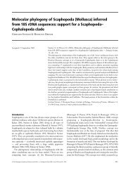
Fig. 1. Power curves for ANOVA design for seagrass west habitat with a. 10 % (n = 118) and b. 25 %
(n = 19) of variability (dispersion coefficient). Dotted line represents the minimum acceptable power of 0.80.
Re-evaluation of data
Figures 1, 2 and 3 show that for the seagrass, rocky shores south and rocky shores west
habitats, respectively, independent of the coefficient of variability, the magnitude of a
possible perturbation (effect size) must always be large, that is ³ 0.40, to ensure a high
robustness of the statistical test (ANOVA) in assessing the hypothesis. In a situation
where the putative perturbation is small (effect size = 0.10), no sample size proposed by
Mouillot et al. (1999) is sufficient. Additionally, if the effect size is < 0.10, more than
1000 samples must be taken for an ANOVA design.

6 Ortiz
Fig. 2. Power curves for ANOVA design for rocky shores south habitat with a. 10 % (n = 112) and b. 25 %
(n = 18) of variability (dispersion coefficient). Dotted line represents the minimum acceptable power of 0.80.
Based on these considerations, it is demonstrated that the procedure for estimating
the sample size is more complex than that proposed by Mouillot et al. (1999). Definitively,
estimating the magnitude of perturbation, i. e. effect sizes, becomes essential not
only to increase the robustness of the statistical test, but also to optimise the costs of the
sampling program. For instance, in a situation with large magnitudes of effect size (e.g.,
0.40) it would only be necessary to have a maximum variability of 25 %. This would
significantly reduce the costs of sampling and study time. Finally, once effect size rates
are roughly estimated, based on previous sampling or a detailed review of the scientific
literature (for comparable situations), a priori power analysis can be implemented to
estimate the optimum sample size (Cohen, 1988; Peterman, 1990a; Underwood, 1997).

Power analysis for sample size estimations 7
Fig. 3. Power curves for ANOVA design for rocky shores east habitat with a. 10 % (n = 130) and b. 25 %
(n = 21) of variability (dispersion coefficient). Dotted line represents the minimum acceptable power of 0.80.
Thus, an incorrect sampling program to assess a potential impact could have negative
consequences on the marine natural systems, especially when the null hypothesis (e.g.,
non-perturbation) was not rejected and simultaneously a posteriori statistical power
was not determined, which finally determines the quality of our conclusions. However,
in those cases when the null hypothesis was not rejected with low power, it is strongly
recommended to use the precautionary principle as an important decision-making tool
for improving management polices.

8 Ortiz
Conclusions
The decrease of the sampling variability (coefficient of variability) is definitively an
excellent and useful strategy to be applied when the magnitude of effect size is small
and, therefore, a large sample size is required. However, this procedure must be applied
once the size of the perturbation is known, not before. Therefore, any sampling program
design should be avoided that could have deleterious consequences for natural systems,
especially when the acceptance of the null hypothesis was incorrect! This situation
could support misguided management plans, as was described extensively by Peterman
(1990a). In conclusion, the magnitude of perturbation (effect size) is the most relevant
information for any hypothesis testing and more efforts must be focused towards its estimation
(Rotenberry & Wiens, 1985).
Acknowledgements
I would like to thank Prof. Dr. M. Wolff, M.Sc. C. Jimenez and Dr. S. Jesse and the anonymous reviewers for
criticising and improving the manuscript.
References
Andrew, N. & B. Mapstone, 1987: Sampling and the description of spatial pattern in marine ecology. Oceanogr.
Mar. Biol. Annu. Rev., 25: 39±90.
Bernstein, B. & J. Zalinski, 1983: An optimum sampling design and power tests for environmental biologists.
J. Environ. Manage., 16: 35±43.
Cohen, J., 1988: Statistical power analysis for the behavioral sciences. 2 nd edition. L. Erlbaum Associates,
Hillsdale, N.Y.; 567 pp.
Dixon, W. & F. Massey, 1969: Introduction to statistical analysis. 3 rd edition. McGraw Hill Book Co., N.Y.;
638 pp.
Gerrodette, T., 1987: A power analysis for detecting trends. Ecology, 68(5): 1364±1372.
Gray, J., 1996: Environmental science and a precautionary approach revisited. Mar. Pollut. Bull., 32(7): 532±
534.
Green, R., 1989: Power analysis and practical strategies for environmental monitoring. Environ. Res., 50:
195±205.
Mapstone, B., 1995: Scalable decision rules for environmental impacts studies: Effect size, Type I and Type II
errors. Ecol. Appl., 5(2): 401±410.
Mouillot, D., J.-M. Culioli, A. Leprete & J.-A. Tomasini, 1999: Dispersion statistics for three fish species
(Symphodus ocellatus, Serranus scriba and Diplodus annularis) in the Lavezzi Islands Marine Reserve
(South Corsica, Mediterranean Sea). P.S.Z.N.: Marine Ecology, 20(1): 19±34.
Peterman, R., 1990a: Statistical power analysis can improve fisheries research and management. Can. J.
Aquat. Sci., 47: 1±15.
Peterman, R., 1990b: The importance of reporting statistical power: the forest decline and acidic deposition
example. Ecology, 71(5): 2024±2027.
Peterman, R. & M. M'Gonigle, 1992: Statistical power analysis and the precautionary principle. Mar. Pollut.
Bull., 24(5): 231±234.
Ribic, Ch. & L. Ganio, 1996: Power analysis for beach surveys of marine debris. Mar. Pollut. Bull., 32(7):
554±557.
Rotenberry, J. & J. Wiens, 1985: Statistical Power Analysis and community-wide patterns. Am. Nat., 125:
164±168.
Schlese, W. & W. Nelson, 1996: A power analysis of methods for assessment of change in seagrass cover.
Aquat. Bot., 53: 227±233.
Sheppard, Ch., 1999: How large should my sample be? Some quick guides to sample size and the power of
test. Mar. Pollut. Bull., 38(6): 439±447.
Sokal, R. & F. Rohlf, 1995: Biometry. 3 rd edition. W.H. Freeman and Co., San Francisco; 878 pp.
Tiku, M., W. Tan & N. Balakrishnan, 1986: Robust Inference. Marcel Dekker, Inc., N.Y.; 321 pp.

Power analysis for sample size estimations 9
Toft, K. & P. Shea, 1983: Detecting community-wide patterns: Estimating power strengthens statistical inference.
Am. Nat., 122(5): 618±625.
Underwood, A., 1981: Techniques of analysis of variance in experimental marine biology and ecology. Oceanogr.
Mar. Biol. Annu. Rev., 19: 513±605.
Underwood, A., 1991: Beyond BACI: experimental designs for detecting human environmental impacts on
temporal variations in natural populations. Aust. J. Mar. Freshwater Res., 42: 569±587.
Underwood, A., 1993: The mechanics of spatially replicated sampling programmes to detect environmental
impacts in a variable world. Aust. J. Ecol., 18: 99±117.
Underwood, A., 1994: On beyond BACI: Sampling designs that might reliably detect environmental disturbances.
Ecol. Appl., 4(1): 3±15.
Underwood, A., 1996: Detection, interpretation, prediction and management of environmental disturbances:
some roles for experimental marine ecology. J. Exp. Mar. Biol. Ecol., 200: 1±27.
Underwood, A., 1997: Experiments in ecology: Their logical design and interpretation using analysis of variance.
Cambridge University Press; 504 pp.
Winer, B., 1971: Statistical principles in experimental design. McGraw-Hill, N.Y.; 907 pp.