Machine Learning, Neural and Statistical Classification - Arteimi.info

Machine Learning, Neural and Statistical 

Classification 

Editors: D. Michie, D.J. Spiegelhalter, C.C. Taylor 

February 17, 1994

Contents 

¡¡ ¢ ¡¡ ¤ ¡ ¡ ¡ ¡ ¢ £ ¢ ¡ ¡ ¡ £ ¢ ¢ ¡ ¡ ¡ £ ¡ ¢ ¡ ¢ ¡ 

¡ ¡ ¡ ¡ ¡ ¢ ¡ ¢ ¡¡ ¢ ¡¡ ¢ ¡ £ ¡ ¢ ¡ ¢ ¡ ¢ £ ¤ £ ¡ ¡ 

¡ ¡ ¢ ¢ ¡¡¡ ¢ ¡ £ ¡ ¡ ¢ ¢ ¡ ¡ 

¡ ¢ ¡¡¡ ¢ ¡¡ ¢ ¡ £ ¤ ¡ £ ¢ ¡ ¡ ¢ ¡ ¢ ¡¡ ¡ ¤ ¢ £ ¡¡¡ ¢ ¡ ¢ ¡¡¡ ¢ ¡¡ ¢ ¡ £ ¡ ¢ ¡ ¡ £ 

¡ ¢ ¡¡ ¢ ¡ ¡ ¡ ¡ £ ¡ ¤ ¢ £ ¡ ¢ ¡¡¡ ¢ ¡¡ ¢ ¡ £ 

¢ ¡¡ ¢ ¡ £ ¡ ¢ ¡¡ ¢ ¡¡ ¡ ¡ ¢ ¢ ¡¡ £ ¤ £ ¡ ¢ ¡¡¡ ¡¡ ¢ ¡ £ ¡ ¢ ¡¡ ¢ ¡¡¡ ¢ £ ¤ £ ¡ ¢ ¡¡¡ ¢ 

¡ ¢ £ ¡ ¤ ¡¡ ¢ ¡¡ ¢ ¡ £ ¡ ¢ ¡¡ ¢ ¡¡¡ ¢ ¢ £ ¡ ¡ 

¡ ¢ ¡ £ ¡ ¡ ¡ ¢ ¢ ¡ 

¡ ¢ ¡¡ ¢ ¡ £ ¡ ¢ ¡¡ ¢ ¡¡¡ ¢ 

1 Introduction 1 

1.1 INTRODUCTION 1 

1.2 CLASSIFICATION 1 

1.3 PERSPECTIVES ON CLASSIFICATION 2 

1.3.1 Statistical approaches 2 

1.3.2 Machine learning 2 

1.3.3 Neural networks 3 

1.3.4 Conclusions 3 

1.4 THE STATLOG PROJECT 4 

1.4.1 Quality control 4 

1.4.2 Caution in the interpretations of comparisons 4 

1.5 THE STRUCTURE OF THIS VOLUME 5 

¡¡¡ ¢ ¡¡ ¢ £ ¢ ¡ ¡ ¡ ¡ ¡ ¡ ¡ ¢ ¢ 

¡ ¡ ¡ ¡ ¢ £ ¢ ¡ ¡ ¡ ¢ ¡ ¢ ¡¡ ¡ ¡ ¡ ¢ ¢ £ £ ¢ ¡ ¡ ¢ ¡ ¤ ¡ 

¡¡ £ ¤ £ ¡ ¡ ¢ ¢ ¡ ¡¡¡ ¢ ¡¡ ¢ ¡ £ ¡ ¢ ¡¡ ¢ ¡¡¡ ¢ ¡ ¢ 

¡¡¡ ¢ ¡¡ ¡ ¢ ¡ ¡ £ £ ¤ ¡ ¢ ¡¡ ¢ ¡¡¡ ¢ £ ¡ ¢ 

¡¡¡ ¢ ¢ ¡¡ £ ¤ £ ¡ ¢ ¡¡¡ ¢ ¡¡ ¢ ¢ ¡ ¡ ¡ £ ¡ ¢ ¡¡ ¢ 

¡¡ ¢ ¡¡ ¢ ¡ £ ¡ ¢ ¡¡ ¢ ¡¡¡ £ ¢ ¡ ¢ ¡ 

¡ ¡ ¡ ¢ ¡¡ ¢ ¡ £ ¡ ¢ ¡¡ ¢ ¡¡¡ ¢ ¢ 

¡ ¢ ¡ ¡ ¢ ¡ ¡ ¢ £ ¡¡¡ ¢ ¡ 

¢ £ ¡ ¤ ¡ £ ¢ ¡ ¡ ¢ ¡ ¡ ¡ ¡ ¢ ¡ ¢ ¡¡ ¢ ¡ £ ¡ 

¡ ¢ ¡¡ ¢ ¡ ¡ £ £ ¡ ¤ ¢ ¡¡ ¢ ¡¡¡ ¢ £ ¡ ¢ ¡¡ ¡¡¡ ¢ ¡ ¢ ¡¡ ¢ 

¢ ¡ ¢ ¡¡¡ ¢ ¡ ¡ ¢ ¡ ¡ £ ¡ ¢ ¡¡ ¢ ¡¡¡ ¢ 

¡ ¢ ¡ £ ¡ ¢ ¡¡ ¢ ¡¡¡ ¢ 

2 Classification 6 

2.1 DEFINITION OF CLASSIFICATION 6 

2.1.1 Rationale 6 

2.1.2 Issues 7 

2.1.3 Class definitions 8 

2.1.4 Accuracy 8 

2.2 EXAMPLES OF CLASSIFIERS 8 

2.2.1 Fisher’s linear discriminants 9 

2.2.2 Decision tree and Rule-based methods 9 

2.2.3 k-Nearest-Neighbour 10 

2.3 CHOICE OF VARIABLES 11 

2.3.1 Transformations and combinations of variables 11 

2.4 CLASSIFICATION OF CLASSIFICATION PROCEDURES 12 

2.4.1 Extensions to linear discrimination 12 

2.4.2 Decision trees and Rule-based methods 12

¦ 

ii [Ch. 0 

2.5 A GENERAL STRUCTURE FOR CLASSIFICATION PROBLEMS 12 

2.5.1 Prior probabilities and the Default rule 13 

2.5.2 Separating classes 13 

2.5.3 Misclassification costs 13 

BAYES RULE GIVEN DATA 14 

2.6.1 Bayes rule in statistics 15 

2.7 REFERENCE TEXTS 16 

¡¡ ¢ ¡¡ £ ¤ ¡ ¡ ¡ ¡ ¢ £ ¢ ¡ ¡ ¡ £ ¡ ¡ ¡ ¢ ¢ ¢ ¡ ¢ ¡ ¡ 

¢ ¡ ¢ ¡ £ ¤ £ ¡ ¢ £ ¢ ¡ ¡ ¡ ¢ ¡ ¡ ¡ ¡ ¡ ¢ ¡ ¡ 

¡ ¢ ¡ ¡ ¡ ¢ ¡ ¡ £ ¡ ¡ ¢ ¢ ¡ 

¢ £ ¢ ¡ ¡ ¡ ¡ ¢ ¡ ¡ ¡ ¡ ¡ ¢ ¡ ¢ ¡ ¡ ¢ ¡ 

¡ ¢ ¡¡¡ ¢ ¢ ¡ ¡ £ 

¢ ¡ £ ¡ ¢ ¤ ¡ £ ¡ ¡ ¢ ¢ ¡ ¡ ¡ ¡ ¡ ¡ ¢ ¢ ¡¡ ¢ ¢ ¡¡ ¢ £ ¡ ¡ £ ¢ ¡ ¡ ¢ ¡ ¡ ¡ ¡ ¢ ¡¡¡ ¡ ¢ ¡¡ ¢ ¡¡¡ ¢ £ 

¡ ¢ ¡ ¢ ¡ ¡ ¡ ¢ ¢ ¡ ¡ £ ¡ 

¢ ¡¡ ¢ ¡¡¡ ¢ ¢ ¡¡ ¢ ¡ £ ¡ 

¡ £ ¢ ¡ £ ¡ ¢ ¡¡ ¢ ¡¡¡ ¡ ¢ ¡ ¡ ¢ ¢ ¤ ¡ ¡ 

¢ ¡ ¡¡ ¢ ¡¡¡ ¢ ¡ £ 

¡ £ ¡ ¢ ¡¡ ¢ ¡¡¡ £ ¢ ¢ ¤ ¡ £ ¡ ¡ ¢ ¢ ¡ ¡ ¡ ¡¡ ¢ ¡¡ ¢ 

¡¡¡ ¢ ¡¡ ¢ ¡ £ ¡ ¢ ¡ ¡ £ ¡ ¡ ¢ ¢ ¡ ¡ ¡ ¡ ¡ ¢ ¢ ¡¡ £ ¤ £ ¡ ¢ 

¡ ¢ ¡¡ £ ¢ ¤ ¡ £ £ ¡ ¡ ¢ ¡¡ ¢ ¡¡¡ ¢ ¢ ¡¡ ¡ ¢ ¡¡¡ ¢ ¡¡ ¢ ¡ £ ¡ ¢ ¡¡ ¢ ¡¡ £ ¡ ¤ ¢ £ 

¤ £ ¡ ¢ ¡¡¡ ¢ ¡¡ ¢ ¡ £ ¡ ¢ ¡¡ ¢ ¡¡¡ ¢ 

3 Classical Statistical Methods 17 


3.2 LINEAR DISCRIMINANTS 17 

3.2.1 Linear discriminants by least squares 18 

3.2.2 Special case of two classes 20 

3.2.3 Linear discriminants by maximum likelihood 20 

3.2.4 More than two classes 21 

3.3 QUADRATIC DISCRIMINANT 22 

3.3.1 Quadratic discriminant - programming details 22 

3.3.2 Regularisation and smoothed estimates 23 

3.3.3 Choice of regularisation parameters 23 

3.4 LOGISTIC DISCRIMINANT 24 

3.4.1 Logistic discriminant - programming details 25 

3.5 BAYES’ RULES 27 

3.6 EXAMPLE 27 

3.6.1 Linear discriminant 27 

3.6.2 Logistic discriminant 27 

3.6.3 Quadratic discriminant 27 

¡¡ ¢ ¡¡ £ ¤ ¡ ¡ ¡ ¡ ¢ £ ¢ ¡ ¡ ¡ £ ¡ ¡ ¡ ¢ ¢ ¢ ¡ ¢ ¡ ¡ 

¡ ¡ ¡ ¡ ¡¡¡ ¢ ¡ ¢ £ ¢ ¢ ¢ ¡ ¤ £ ¡ ¡ ¡ ¡ ¡ ¢ £ 

¡¡ £ ¤ £ ¡ ¢ ¢ ¡ ¡ ¡ ¡ ¡ ¢ ¡¡ ¢ ¡ £ ¡ ¢ ¡¡ ¢ ¡¡¡ ¢ ¢ 

¢ ¡¡¡ ¢ ¡¡ ¢ ¡ -NEAREST £ NEIGHBOUR ¡ ¢ ¡¡ ¢ ¡¡¡ ¢ 35 

¤ £ ¡ 

¡¡ ¢ ¡ ¢ ¡¡ £ ¤ £ ¡ ¢ ¡¡¡ ¢ ¡ ¢ ¡ ¡ ¢ ¡ £ ¡ ¢ ¡¡ ¢ ¡ 

¡ ¢ ¡¡ ¢ ¡ £ ¡ ¢ ¡¡ ¢ ¡¡ ¢ ¡ ¡ ¡ ¡ ¢ ¡ ¡¡¡ ¢ ¡ £ ¢ ¤ ¢ £ ¡ ¢ ¡¡¡ ¢ ¡¡ ¢ ¡ £ ¡ 

¢ ¡ £ ¡ ¢ ¡¡ ¢ 4.5 ¡¡ ¢ ¡ ¡ ¢ ¡ ¢ ¡¡ £ ¤ £ ¡ ¢ ¡¡¡ ¢ ¡¡ £ ¡ ¢ ¡¡ ¢ ¡¡¡ ¢ ¡¡ £ ¤ £ ¡ ¢ ¡¡¡ ¢ ¡¡ ¢ ¡ 

¡¡¡ ¢ ¡¡ ¢ ¡ £ ¡ ¢ ¡¡ ¢ ¡¡¡ ¢ ¢ ¡ ¡ ¡ ¡ £ ¢ ¤ £ ¡ ¢ 

¢ ¡ £ ¡ ¢ ¡¡ ¢ ¡¡¡ ¢ ¡ ¡ ¡ ¢ ¢ ¡ ¡¡ £ ¤ £ ¡ ¢ ¡¡¡ ¡ ¢ ¡ ¡ ¢ ¡ ¡ ¢ ¡ ¡ £ ¡ ¢ ¡¡ ¢ ¡¡¡ ¢ ¢ ¡¡ ¡ ¢ ¡¡ £ ¤ £ ¡ ¡ ¢ ¢ ¡ ¡¡¡ ¢ ¡¡ ¢ ¡ £ ¡ ¢ ¡¡ ¢ ¡¡¡ ¢ 

4 Modern Statistical Techniques 29 


4.2 DENSITY ESTIMATION 30 

4.2.1 Example 33 

4.3 


4.4 PROJECTION PURSUIT CLASSIFICATION 37 


NAIVE BAYES 40 

4.6 CAUSAL NETWORKS 41 


4.7 OTHER RECENT APPROACHES 46 

4.7.1 ACE 46 

4.7.2 MARS 47

Sec. 0.0] 

iii 

¡¡ ¢ ¡¡¡ ¢ 

¡ ¢ ¡¡ ¢ ¡ £ ¡ ¢ ¡ ¡ ¡ ¡ ¡ ¢ ¢ 

¢ ¡ ¡ ¢ ¡ ¡ ¡ ¢ 

¢ ¡ ¢ ¡ ¡ ¢ ¡¡ £ ¤ £ ¡ ¡ ¡ ¡ £ ¢ ¡ ¡ ¢ ¢ ¡ ¡ ¡ ¡ ¢ 

¢ ¡¡ ¡¡ ¢ ¡ ¢ ¡ 

¢ ¡ ¢ ¡ ¡ ¡ ¡ ¢ ¢ ¡ ¡ £ 

¡ ¢ ¡¡ ¢ ¡ ¡ ¡ ¡ ¡ ¢ ¡¡ ¤ ¡ ¡ ¡ ¡ £ £ ¢ ¢ ¡ £ ¢ 

¢ ¡ ¡ ¢ ¡ ¡¡ ¢ ¡¡¡ ¢ ¢ ¡ ¡ ¢ ¡ ¡ ¡ £ 

¢ ¡ ¡ ¢ ¡ ¡ £ ¡ ¢ ¡¡ ¢ ¡¡¡ ¢ ¡ ¢ ¡ ¡ 

¢ ¡ £ ¡ ¢ ¡¡ ¢ ¡¡¡ ¢ ¡¡ ¤ £ ¡ ¢ ¡¡¡ ¢ ¡¡ ¢ ¡ £ ¡ ¢ ¡¡ ¢ ¡ ¡ ¡ ¡ ¡ ¢ ¢ ¡ ¡ ¢ ¡ £ 

¢ ¢ ¡¡¡ ¢ ¡¡ £ ¤ £ ¡ ¢ ¡¡¡ ¢ ¡¡ ¢ ¡ §£¨¢© £ ¡ ¡ ¡ ¢ ¢ ¡ ¡ ¡ ¡ 

¡¡ ¢ ¡ £ ¡ ¡ ¢ ¢ ¡ ¡¡ ¢ ¡¡¡ ¢ ¡¡ ¢ 

¢ ¡ ¡ ¡ ¡ ¢ ¡¡¡ ¢ ¢ ¡¡ ¢ ¡¡ £ ¤ £ ¡ ¢ ¡¡¡ ¢ ¡¡ ¢ ¡ £ ¡ 

¡¡ ¢ ¡¡¡ ¡ ¢ ¡ ¢ ¡¡ £ ¤ £ ¡ ¢ ¡¡¡ ¢ ¡¡ ¢ ¡ £ ¡ ¢ 

¡ ¢ ¢ ¡ ¡ ¡ ¡ ¢ ¡ £ ¡ ¢ ¡¡ ¢ ¡¡ ¡¡¡ ¢ ¡¡ ¢ ¡ £ ¡ ¢ ¡¡ ¢ ¡¡¡ ¢ ¡ ¢ ¡¡ £ ¡ ¤ ¢ £ ¡ ¡ ¢ 

¢ ¡ ¡ ¡ ¡ ¢ ¢ ¡ £ ¡ ¢ ¡¡ ¢ ¡ 

¡¡¡ ¢ ¡¡ ¢ ¡ £ ¡ ¢ ¡¡ ¢ ¡¡¡ ¢ ¢ ¡¡ £ ¤ £ ¡ ¢ 

¡ ¡ ¢ ¢ ¡ £ ¡ ¢ ¡¡ ¢ ¡¡¡ ¢ ¡ ¡ ¡ 

¡¡ ¢ ¡ £ ¡ ¡ ¡ ¢ ¢ 

¡ ¢ ¡¡¡ ¢ 

5 Machine Learning of Rules and Trees 50 

5.1 RULES AND TREES FROM DATA: FIRST PRINCIPLES 50 

5.1.1 Data fit and mental fit of classifiers 50 

5.1.2 Specific-to-general: a paradigm for rule-learning 54 

5.1.3 Decision trees 56 

5.1.4 General-to-specific: top-down induction of trees 57 

5.1.5 Stopping rules and class probability trees 61 

5.1.6 Splitting criteria 61 

5.1.7 Getting a “right-sized tree” 63 

5.2 STATLOG’S ML ALGORITHMS 65 

5.2.1 Tree-learning: further features of C4.5 65 

5.2.2 NewID 65 

5.2.3 67 

5.2.4 Further features of CART 68 

5.2.5 Cal5 70 

5.2.6 Bayes tree 73 

5.2.7 Rule-learning algorithms: CN2 73 

5.2.8 ITrule 77 

5.3 BEYOND THE COMPLEXITY BARRIER 79 

5.3.1 Trees into rules 79 

5.3.2 Manufacturing new attributes 80 

5.3.3 Inherent limits of propositional-level learning 81 

5.3.4 A human-machine compromise: structured induction 83 

¡¡ ¢ ¡¡ £ £ ¢ ¡ ¢ ¡ ¡ ¡ ¡ ¢ ¡ ¢ ¡ ¡ ¢ ¢ ¡ ¤ ¡ ¡ ¡ ¡ £ 

¡¡¡ ¢ ¢ ¢ ¡ ¡ ¡ 

£ ¢ ¡ ¡ ¡ ¡ ¡ ¢ ¢ ¡ ¢ ¡ 

¢ ¢ ¡ ¡ ¢ ¡ ¡ ¡ 

¢ £ ¢ ¡¡ ¢ ¡¡ ¢ ¡ ¡ ¡ ¡ ¡ ¡ ¢ ¡ 

¡¡¡ ¢ ¢ 

¡ ¢ ¡ ¡ ¢ ¢ ¡ ¡ ¡ ¡ ¢ £ ¡ £ ¡ ¢ ¡¡ ¢ ¡¡ ¡ ¢ ¢ ¡ ¡ ¡ ¡ ¢ ¢ ¡ ¡ £ ¡ ¡ ¡ ¢ 

¡ ¡ ¡ ¡ ¢ ¢ ¡ 

¡ ¡ ¡ ¡ £ ¢ ¤ £ ¡ ¢ ¡¡¡ ¢ ¡¡ ¢ ¡ £ ¡ ¢ ¡ ¡ ¡ ¡ ¢ ¢ ¡ 

¡ ¡ ¢ ¡ ¡ ¢ ¡ ¡ ¢ £ ¡ ¢ ¡¡ ¢ ¡¡ ¡ ¡ ¡ ¢ £ ¤ £ ¡ ¢ ¡ ¤ ¡ £ ¡ ¡ ¢ 

¡ ¢ ¡¡ ¢ ¡ £ ¡ ¢ ¡¡ ¢ ¡¡¡ ¢ ¡ ¢ ¡¡ £ ¤ £ ¡ ¢ ¡¡ ¢ ¡ £ ¡ ¢ ¡¡ ¢ ¡¡¡ ¢ ¡ ¢ ¡ ¡ ¡ ¢ ¡¡ ¢ ¡¡ ¢ ¡ £ ¡ ¢ ¡¡ £ ¢ ¤ ¡ £ ¡¡ ¢ ¡ ¢ ¡¡¡ ¡¡¡ ¢ ¡¡ ¢ ¡ £ ¡ ¢ ¡¡ ¢ ¡¡¡ ¢ £ ¤ £ ¡ ¢ 

¡ ¢ ¢ £ ¡ ¡ ¡ ¢ ¡¡¡ ¢ 

6 Neural Networks 84 


6.2 SUPERVISED NETWORKS FOR CLASSIFICATION 86 

6.2.1 Perceptrons and Multi Layer Perceptrons 86 

6.2.2 Multi Layer Perceptron structure and functionality 87 

6.2.3 Radial Basis Function networks 93 

6.2.4 Improving the generalisation of Feed-Forward networks 96 

6.3 UNSUPERVISED LEARNING 101 

6.3.1 The K-means clustering algorithm 101 

6.3.2 Kohonen networks and Learning Vector Quantizers 102 

6.3.3 RAMnets 103 

6.4 DIPOL92 103 

6.4.1 Introduction 104 

6.4.2 Pairwise linear regression 104 

6.4.3 Learning procedure 104 

6.4.4 Clustering of classes 105 

6.4.5 Description of the classification procedure 105

iv [Ch. 0 

¡¡ ¢ 

¢ ¡¡ £ ¤ £ ¡ ¢ ¡¡ ¢ ¡ ¡¡ £ ¢ ¡ ¡ ¡ ¢ ¡ ¢ ¢ ¡ ¡ ¡ 

¡ ¡¡ £ ¡ ¡ ¡ ¤ ¡ ¡ ¡ ¡ ¢ ¡ ¡ ¡ £ ¡ ¡ ¢ ¢ ¢ ¢ £ ¢ 

¡ ¡ ¡ ¡ ¢ £ ¡ ¢ ¡ ¢ ¡ ¢ ¡ ¤ ¢ ¢ ¡ ¡ ¡ ¡ £ ¡ ¡ ¡ £ ¢ ¡ ¡ 

¡ ¢ ¡¡ ¢ ¡ £ ¡ ¢ ¡¡ ¢ ¡¡¡ ¢ ¢ ¡¡ ¢ ¡¡¡ ¢ ¡ ¢ £ ¡ ¢ ¡ ¡ 

¢ ¢ ¡¡¡ ¢ ¡¡ ¢ ¡ ¡ £ ¡ ¡ £ ¢ ¤ ¡ £ ¡ ¡ ¢ ¡¡¡ £ ¡ ¢ ¡¡ ¢ ¡¡¡ ¢ ¡¡ £ ¤ £ ¡ ¡ ¡ ¢ ¢ ¡¡¡ ¢ ¡¡ ¢ ¡ 

¡¡ ¢ ¡ ¢ ¡¡¡ £ ¢ ¤ ¡ £ ¡ ¢ ¡ £ ¡ ¢ ¡¡ ¢ ¡ 

¢ ¡¡¡ ¢ ¡ ¢ ¡¡ ¢ ¡ £ ¡ ¢ ¡¡ ¡ £ ¡ ¢ ¡¡ ¢ ¡¡¡ ¢ ¡ £ ¡ ¤ £ ¡ ¢ ¡¡¡ ¢ ¡¡ ¢ 

¢ ¡ £ ¡ ¢ ¡¡ ¢ ¡¡¡ ¢ ¡ £ ¢ £ ¡ ¤ ¡¡ ¢ ¡¡ ¡¡¡ ¢ ¡ ¢ ¡ ¡¡ ¢ ¡ £ ¡ ¢ ¡¡ ¢ 

¢ £ ¤ £ ¡ ¢ ¡¡¡ ¡ ¢ ¢ ¡ ¡ ¡ ¡ ¢ ¡ £ ¡ ¢ ¡¡ ¢ ¡¡¡ ¢ ¡¡¡ ¢ £ ¡ ¢ ¡¡¡ ¢ ¢ ¡ ¡ ¡ ¡ ¢ £ ¡ ¤ £ ¡ ¢ ¡¡ ¡ ¢ ¡ £ ¡ ¡ ¡ ¢ ¢ ¡¡ ¢ ¡¡¡ ¢ ¡ 

¢ ¢ ¡¡¡ ¢ ¡¡ ¢ ¡ £ ¡ ¢ ¡¡ ¢ ¡¡¡ ¡¡ ¢ ¡¡¡ ¢ ¡ ¡ £ ¡ ¢ ¡ ¢ ¡¡ ¢ ¡ £ ¡ ¢ 

£ ¡ ¡ ¢ ¢ ¡ ¡ ¡ ¡ ¢ ¡¡¡ ¢ ¡ ¢ ¡¡ ¢ ¤ ¡ £ 

¡¡ ¢ ¡ ¤ £ £ ¡ ¡ ¢ ¢ ¡ ¡ ¡ ¡ ¢ ¡¡¡ ¢ ¡ ¢ 

¡¡ ¢ ¡ £ ¡ ¢ ¡¡ ¢ ¡¡¡ ¡ ¢ ¢ 

7 Methods for Comparison 107 

7.1 ESTIMATION OF ERROR RATES IN CLASSIFICATION RULES 107 

7.1.1 Train-and-Test 108 

7.1.2 Cross-validation 108 

7.1.3 Bootstrap 108 

7.1.4 Optimisation of parameters 109 

7.2 ORGANISATION OF COMPARATIVE TRIALS 110 

7.2.1 Cross-validation 111 

7.2.2 Bootstrap 111 

7.2.3 Evaluation Assistant 111 

7.3 CHARACTERISATION OF DATASETS 112 

7.3.1 Simple measures 112 

7.3.2 Statistical measures 112 

7.3.3 Information theoretic measures 116 

7.4 PRE-PROCESSING 120 

7.4.1 Missing values 120 

7.4.2 Feature selection and extraction 120 

7.4.3 Large number of categories 121 

7.4.4 Bias in class proportions 122 

7.4.5 Hierarchical attributes 123 

7.4.6 Collection of datasets 124 

7.4.7 Preprocessing strategy in StatLog 124 

¡¡ ¢ ¡¡ £ ¤ £ ¡ ¡ ¡ ¡ ¢ £ ¢ ¡ ¡ ¡ ¢ ¢ ¡ ¡ ¡ ¡ ¡ ¢ ¢ ¡ 

¡ ¢ £ ¡¡ ¢ ¡¡ ¢ ¡ ¢ ¡ ¡ ¡ ¡ ¡ ¢ 

¡¡¡ ¢ ¢ ¡¡ ¢ ¡ £ ¡ ¢ ¡¡ ¢ 

£ ¡ ¢ ¡¡ ¢ ¡¡¡ ¢ ¡ ¢ ¢ ¡ ¡ 

¡ ¢ ¡¡ ¢ ¡¡¡ ¢ ¢ ¡ ¡ £ ¡ ¤ ¡ £ ¢ ¡ ¡¡ ¢ ¡ £ 

£ ¢ ¡ ¡ ¡ ¡ ¢ ¡¡¡ ¢ 

¡¡ ¢ ¡¡¡ ¢ ¡ ¢ 

¢ ¡¡¡ ¡ ¡ ¢ £ ¡ ¡ ¡ ¡ ¡ ¢ ¢ ¡ ¡ ¢ 

¡ ¢ ¡¡ ¢ ¡ ¡ ¡ ¢ ¡ ¡ ¢ £ 

8 Review of Previous Empirical Comparisons 125 


8.2 BASIC TOOLBOX OF ALGORITHMS 125 

8.3 DIFFICULTIES IN PREVIOUS STUDIES 126 

8.4 PREVIOUS EMPIRICAL COMPARISONS 127 

8.5 INDIVIDUAL RESULTS 127 

8.6 MACHINE LEARNING vs. NEURAL NETWORK 127 

8.7 STUDIES INVOLVING ML, k-NN AND STATISTICS 129 

8.8 SOME EMPIRICAL STUDIES RELATING TO CREDIT RISK 129 

8.8.1 Traditional and statistical approaches 129 

8.8.2 Machine Learning and Neural Networks 130 

¡¡ ¢ ¡¡ £ ¤ £ ¢ ¡ ¢ ¡ ¡ ¡ ¡ ¢ ¡ ¢ ¡ ¡ £ ¡ ¡ ¡ ¢ ¡ ¡ ¢ 

¡ ¡ ¢ ¡ ¢ £ ¢ ¡¡¡ ¢ ¡ ¢ ¡ £ ¢ ¡ ¡ ¡ ¤ ¡ ¢ ¡¡ £ ¡ 

¡ ¡ ¢ ¡ ¡ ¢ ¡ ¡ ¡ ¡ ¢ ¢ ¡ £ ¡ ¢ ¡ 

¡¡ ¢ ¡¡ ¢ ¡ £ ¡ ¢ ¡¡ ¢ ¡ ¡ ¡ ¢ ¡ ¡ ¢ 

¡ ¢ ¡¡ ¡ ¢ ¢ ¡ ¡ ¡ ¡ ¡ ¢ £ ¤ £ ¡ ¢ ¡¡¡ ¢ ¡¡ ¢ ¡ £ 

¡ ¢ ¡¡¡ ¢ ¡ ¢ ¡¡¡ ¢ ¡¡ ¢ ¡ £ ¡ ¢ ¡ 

¢ ¡ ¢ ¡¡ ¢ ¡¡¡ ¢ ¡ ¢ ¡ ¡ ¢ ¡ ¡ ¡ £ 

£ ¡ ¢ ¢ ¡ ¡ ¡ ¡ ¢ ¡ ¡ ¢ ¡¡ ¢ ¡¡ ¢ ¡ 

¡ ¢ ¡¡ ¢ ¡ £ ¡ ¢ ¡¡ ¢ ¡ ¡ ¡ ¢ ¡ ¡ ¢ ¡ 

9 Dataset Descriptions and Results 131 


9.2 CREDIT DATASETS 132 

9.2.1 Credit management (Cred.Man) 132 

9.2.2 Australian credit (Cr.Aust) 134 

9.3 IMAGE DATASETS 135 

9.3.1 Handwritten digits (Dig44) 135 

9.3.2 Karhunen-Loeve digits (KL) 137 

9.3.3 Vehicle silhouettes (Vehicle) 138 

9.3.4 Letter recognition (Letter) 140

Sec. 0.0] 

v 

£ ¡ ¢ ¡ ¢ ¡ ¡ ¡ ¡ ¢ ¡ ¢ ¡ ¢ ¢ ¡ ¡ £ ¡ ¡ ¡ 

¡ ¡ ¡ ¢ ¡ £ ¡ ¡ ¢ ¢ ¡¡ ¡ ¢ ¢ ¡ ¡ 

¡¡¡ ¢ ¢ ¡ ¢ ¡ ¡ £ ¢ ¡ ¡ ¢ ¡ ¡ ¢ ¡ ¡ 

¡ £ ¡¡ ¢ ¡ ¡ ¡ ¡ ¢ ¡ ¢ ¡ ¢ ¡ ¤ ¢ ¡ ¡ £ ¡ ¡ ¡ £ ¡ ¢ ¡ ¡ ¡ ¢ ¢ £ 

¢ ¡ ¢ ¡ ¡ ¡ ¡¡ ¢ ¡¡¡ ¡ ¢ £ ¢ £ ¤ £ ¡ ¢ ¡ ¡ 

¢ ¡¡ ¢ ¡ £ ¡ ¢ ¡¡ ¢ ¡¡ ¡ ¡ £ ¢ ¤ £ ¡ ¢ ¡¡¡ ¡ ¢ ¡¡ ¢ ¡ £ ¡ ¢ ¡¡ ¢ ¡¡¡ ¢ ¤ £ £ ¡ ¢ ¡¡ ¡ ¢ ¡ £ ¡ ¢ ¡¡ ¢ ¡¡¡ ¢ ¡ ¡ ¡ ¢ ¢ ¡ ¡ £ 

¡ ¡ £ ¢ ¡ £ ¡ ¢ ¡¡ ¢ ¡¡¡ ¢ ¤ £ ¡ ¢ ¡¡ ¡ ¡ ¢ ¢ ¡ ¡ 

¢ ¡¡ ¢ ¡¡ ¢ £ ¡ ¡ £ ¢ ¡ ¡ ¢ ¡¡ ¢ ¡¡¡ ¡ ¢ ¡ £ ¡ ¢ ¡¡ ¡ ¢ ¡ ¡ £ ¡ ¤ ¡ £ ¢ ¡ ¢ ¡¡¡ ¢ ¡ 

¢ ¡ ¡¡ ¢ ¡¡¡ ¢ ¡ ¢ ¡¡ £ ¤ £ ¡ ¢ ¡¡¡ ¢ ¡¡ ¢ ¡ ¡ £ ¡ ¡ ¢ 

¤ £ ¡ ¢ ¡¡¡ ¢ ¡¡ ¢ ¡ £ ¡ ¢ ¡ ¡ ¡ ¡ ¢ £ ¡¡¡ ¢ 

¡ ¢ ¡¡ ¢ ¡ £ ¡ ¢ ¡¡ ¢ ¡¡¡ ¢ ¤ £ ¡ ¢ ¡¡ ¡ ¢ ¡ ¡ £ ¡ ¢ ¡¡ ¢ ¡¡¡ ¢ ¡ ¢ ¡ ¡ ¢ ¡ 

¡¡ ¢ ¡¡ ¢ ¡¡ ¢ ¡ £ ¡ ¢ ¤ ¡ £ ¡ ¡ ¢ ¢ ¡ ¡ 

¡ ¢ ¡ £ ¡ ¢ ¡¡ ¢ ¡¡¡ ¢ ¡¡¡ ¢ ¡ 

¡ ¡ ¡¡ ¢ £ ¡ ¢ ¢ ¡ 

¢ ¡¡ ¢ ¡ £ ¡ ¢ ¡ ¡ ¡ ¡ £ ¢ ¤ ¡ £ ¡¡ ¢ ¡ ¢ ¡¡¡ ¡¡¡ ¢ ¡¡ ¢ ¡ £ ¡ ¢ ¡¡ ¢ ¡ ¡ £ ¡ ¤ ¡ £ ¢ ¡ ¢ 

¡ ¢ ¡ ¡ £ ¡ ¤ ¡ ¢ £ ¡ ¢ ¡¡¡ ¢ ¡¡ ¢ ¡ £ ¡ ¢ ¡ ¡ ¢ ¡ 

¡ ¢ ¡ £ ¡ ¢ ¡¡ ¢ ¡¡¡ ¢ £ ¤ £ ¡ ¢ ¡ ¡ ¢ ¡ ¡ ¡ ¡ ¢ ¡ 

£ ¡ ¡ ¢ ¢ ¡¡ ¢ ¡¡¡ ¢ ¡¡¡ ¢ ¡¡ ¢ ¤ ¡ £ 

¡ ¢ ¡¡ ¢ ¡ £ ¢ ¡ ¡ ¢ ¡ ¡ £ ¡ ¢ ¡¡¡ ¢ ¤ £ ¡ ¢ ¡¡ £ ¤ £ ¡ ¢ ¡¡¡ ¢ ¡¡ ¢ ¡ £ ¡ ¢ ¢ ¡ ¡ ¡ ¡ ¢ ¢ ¡¡¡ ¢ ¡¡ £ ¤ £ ¡ ¢ ¡¡¡ ¢ ¡¡ ¢ ¡ £ ¡ ¢ ¡¡ ¢ ¡¡¡ ¡ ¢ ¡ 

9.3.5 Chromosomes (Chrom) 142 

9.3.6 Landsat satellite image (SatIm) 143 

9.3.7 Image segmentation (Segm) 145 

9.3.8 Cut 146 

9.4 DATASETS WITH COSTS 149 

9.4.1 Head injury (Head) 149 

9.4.2 Heart disease (Heart) 152 

9.4.3 German credit (Cr.Ger) 153 

9.5 OTHER DATASETS 154 

9.5.1 Shuttle control (Shuttle) 154 

9.5.2 Diabetes (Diab) 157 

9.5.3 DNA 158 

9.5.4 Technical (Tech) 161 

9.5.5 Belgian power (Belg) 163 

9.5.6 Belgian power II (BelgII) 164 

9.5.7 Machine faults (Faults) 165 

9.5.8 Tsetse fly distribution (Tsetse) 167 

9.6 STATISTICAL AND INFORMATION MEASURES 169 

9.6.1 KL-digits dataset 170 

9.6.2 Vehicle silhouettes 170 

9.6.3 Head injury 173 

9.6.4 Heart disease 173 

9.6.5 Satellite image dataset 173 

9.6.6 Shuttle control 173 

9.6.7 Technical 174 

9.6.8 Belgian power II 174 

10 Analysis of Results 175 

10.1 INTRODUCTION ¡ ¡ ¢ ¡ ¡ £ ¤ £ ¡ ¢ ¡ ¡ ¡ ¢ ¡ ¡ ¢ ¡ £ ¡ ¢ ¡ ¡ ¢ ¡ ¡ ¡ ¢ 175 

10.2 RESULTS BY SUBJECT AREAS ¡ ¢ ¡ ¡ ¡ ¢ ¡ ¡ ¢ ¡ £ ¡ ¢ ¡ ¡ ¢ ¡ ¡ ¡ ¢ 176 

10.2.1 Credit datasets ¢ ¡ ¡ £ ¤ £ ¡ ¢ ¡ ¡ ¡ ¢ ¡ ¡ ¢ ¡ £ ¡ ¢ ¡ ¡ ¢ ¡ ¡ ¡ ¢ 176 

10.2.2 Image datasets ¢ ¡ ¡ £ ¤ £ ¡ ¢ ¡ ¡ ¡ ¢ ¡ ¡ ¢ ¡ £ ¡ ¢ ¡ ¡ ¢ ¡ ¡ ¡ ¢ 179 

10.2.3 Datasets with costs ¡ £ ¤ £ ¡ ¢ ¡ ¡ ¡ ¢ ¡ ¡ ¢ ¡ £ ¡ ¢ ¡ ¡ ¢ ¡ ¡ ¡ ¢ 183 

10.2.4 Other datasets ¢ ¡ ¡ £ ¤ £ ¡ ¢ ¡ ¡ ¡ ¢ ¡ ¡ ¢ ¡ £ ¡ ¢ ¡ ¡ ¢ ¡ ¡ ¡ ¢ 184 

10.3 TOP FIVE ALGORITHMS £ ¤ £ ¡ ¢ ¡ ¡ ¡ ¢ ¡ ¡ ¢ ¡ £ ¡ ¢ ¡ ¡ ¢ ¡ ¡ ¡ ¢ 185 

10.3.1 Dominators ¡ ¢ ¡ ¡ £ ¤ £ ¡ ¢ ¡ ¡ ¡ ¢ ¡ ¡ ¢ ¡ £ ¡ ¢ ¡ ¡ ¢ ¡ ¡ ¡ ¢ 186 

10.4 MULTIDIMENSIONAL SCALING ¢ ¡ ¡ ¡ ¢ ¡ ¡ ¢ ¡ £ ¡ ¢ ¡ ¡ ¢ ¡ ¡ ¡ ¢ 187 

10.4.1 Scaling of algorithms ¤ £ ¡ ¢ ¡ ¡ ¡ ¢ ¡ ¡ ¢ ¡ £ ¡ ¢ ¡ ¡ ¢ ¡ ¡ ¡ ¢ 188 

10.4.2 Hierarchical clustering of algorithms ¢ ¡ ¡ ¢ ¡ £ ¡ ¢ ¡ ¡ ¢ ¡ ¡ ¡ ¢ 189 

10.4.3 Scaling of datasets ¡ £ ¤ £ ¡ ¢ ¡ ¡ ¡ ¢ ¡ ¡ ¢ ¡ £ ¡ ¢ ¡ ¡ ¢ ¡ ¡ ¡ ¢ 190 

10.4.4 Best algorithms for datasets ¢ ¡ ¡ ¡ ¢ ¡ ¡ ¢ ¡ £ ¡ ¢ ¡ ¡ ¢ ¡ ¡ ¡ ¢ 191 

10.4.5 Clustering of datasets ¤ £ ¡ ¢ ¡ ¡ ¡ ¢ ¡ ¡ ¢ ¡ £ ¡ ¢ ¡ ¡ ¢ ¡ ¡ ¡ ¢ 192 

10.5 PERFORMANCE RELATED TO MEASURES: THEORETICAL ¡ ¡ ¢ 192 

10.5.1 Normal distributions £ ¤ £ ¡ ¢ ¡ ¡ ¡ ¢ ¡ ¡ ¢ ¡ £ ¡ ¢ ¡ ¡ ¢ ¡ ¡ ¡ ¢ 192 

10.5.2 Absolute performance: quadratic discriminants ¡ ¢ ¡ ¡ ¢ ¡ ¡ ¡ ¢ 193

vi [Ch. 0 

10.5.3 Relative performance: Logdisc vs. DIPOL92 £ ¡ ¢ ¡ ¡ ¢ ¡ ¡ ¡ ¢ 193 

10.5.4 Pruning of decision trees £ ¡ ¢ ¡ ¡ ¡ ¢ ¡ ¡ ¢ ¡ £ ¡ ¢ ¡ ¡ ¢ ¡ ¡ ¡ ¢ 194 

10.6 RULE BASED ADVICE ON ALGORITHM APPLICATION ¡ ¢ ¡ ¡ ¡ ¢ 197 

10.6.1 Objectives ¡ ¡ ¢ ¡ ¡ £ ¤ £ ¡ ¢ ¡ ¡ ¡ ¢ ¡ ¡ ¢ ¡ £ ¡ ¢ ¡ ¡ ¢ ¡ ¡ ¡ ¢ 197 

10.6.2 Using test results in metalevel learning ¡ ¡ ¢ ¡ £ ¡ ¢ ¡ ¡ ¢ ¡ ¡ ¡ ¢ 198 

10.6.3 Characterizing predictive power ¡ ¡ ¢ ¡ ¡ ¢ ¡ £ ¡ ¢ ¡ ¡ ¢ ¡ ¡ ¡ ¢ 202 

10.6.4 Rules generated in metalevel learning ¡ ¡ ¢ ¡ £ ¡ ¢ ¡ ¡ ¢ ¡ ¡ ¡ ¢ 205 

10.6.5 Application Assistant ¤ £ ¡ ¢ ¡ ¡ ¡ ¢ ¡ ¡ ¢ ¡ £ ¡ ¢ ¡ ¡ ¢ ¡ ¡ ¡ ¢ 207 

10.6.6 Criticism of metalevel learning approach ¢ ¡ £ ¡ ¢ ¡ ¡ ¢ ¡ ¡ ¡ ¢ 209 

10.6.7 Criticism of measures ¤ £ ¡ ¢ ¡ ¡ ¡ ¢ ¡ ¡ ¢ ¡ £ ¡ ¢ ¡ ¡ ¢ ¡ ¡ ¡ ¢ 209 

10.7 PREDICTION OF PERFORMANCE ¡ ¡ ¡ ¢ ¡ ¡ ¢ ¡ £ ¡ ¢ ¡ ¡ ¢ ¡ ¡ ¡ ¢ 210 

10.7.1 ML on ML vs. regression ¡ ¢ ¡ ¡ ¡ ¢ ¡ ¡ ¢ ¡ £ ¡ ¢ ¡ ¡ ¢ ¡ ¡ ¡ ¢ 211 

11 Conclusions 213 

11.1 INTRODUCTION ¡ ¡ ¢ ¡ ¡ £ ¤ £ ¡ ¢ ¡ ¡ ¡ ¢ ¡ ¡ ¢ ¡ £ ¡ ¢ ¡ ¡ ¢ ¡ ¡ ¡ ¢ 213 

11.1.1 User’s guide to programs £ ¡ ¢ ¡ ¡ ¡ ¢ ¡ ¡ ¢ ¡ £ ¡ ¢ ¡ ¡ ¢ ¡ ¡ ¡ ¢ 214 

11.2 STATISTICAL ALGORITHMS £ ¡ ¢ ¡ ¡ ¡ ¢ ¡ ¡ ¢ ¡ £ ¡ ¢ ¡ ¡ ¢ ¡ ¡ ¡ ¢ 214 

11.2.1 Discriminants ¢ ¡ ¡ £ ¤ £ ¡ ¢ ¡ ¡ ¡ ¢ ¡ ¡ ¢ ¡ £ ¡ ¢ ¡ ¡ ¢ ¡ ¡ ¡ ¢ 214 

11.2.2 ALLOC80 ¡ ¡ ¢ ¡ ¡ £ ¤ £ ¡ ¢ ¡ ¡ ¡ ¢ ¡ ¡ ¢ ¡ £ ¡ ¢ ¡ ¡ ¢ ¡ ¡ ¡ ¢ 214 

11.2.3 Nearest Neighbour ¡ £ ¤ £ ¡ ¢ ¡ ¡ ¡ ¢ ¡ ¡ ¢ ¡ £ ¡ ¢ ¡ ¡ ¢ ¡ ¡ ¡ ¢ 216 

11.2.4 SMART ¢ ¡ ¡ ¢ ¡ ¡ £ ¤ £ ¡ ¢ ¡ ¡ ¡ ¢ ¡ ¡ ¢ ¡ £ ¡ ¢ ¡ ¡ ¢ ¡ ¡ ¡ ¢ 216 

11.2.5 Naive Bayes ¡ ¢ ¡ ¡ £ ¤ £ ¡ ¢ ¡ ¡ ¡ ¢ ¡ ¡ ¢ ¡ £ ¡ ¢ ¡ ¡ ¢ ¡ ¡ ¡ ¢ 216 

11.2.6 CASTLE ¢ ¡ ¡ ¢ ¡ ¡ £ ¤ £ ¡ ¢ ¡ ¡ ¡ ¢ ¡ ¡ ¢ ¡ £ ¡ ¢ ¡ ¡ ¢ ¡ ¡ ¡ ¢ 217 

11.3 DECISION TREES ¡ ¢ ¡ ¡ £ ¤ £ ¡ ¢ ¡ ¡ ¡ ¢ ¡ ¡ ¢ ¡ £ ¡ ¢ ¡ ¡ ¢ ¡ ¡ ¡ ¢ 217 

11.3.1 §£¨¢© and NewID ¡ ¡ £ ¤ £ ¡ ¢ ¡ ¡ ¡ ¢ ¡ ¡ ¢ ¡ £ ¡ ¢ ¡ ¡ ¢ ¡ ¡ ¡ ¢ 218 

11.3.2 C4.5 ¡ ¡ ¢ ¡ ¡ ¢ ¡ ¡ £ ¤ £ ¡ ¢ ¡ ¡ ¡ ¢ ¡ ¡ ¢ ¡ £ ¡ ¢ ¡ ¡ ¢ ¡ ¡ ¡ ¢ 219 

11.3.3 CART and IndCART £ ¤ £ ¡ ¢ ¡ ¡ ¡ ¢ ¡ ¡ ¢ ¡ £ ¡ ¢ ¡ ¡ ¢ ¡ ¡ ¡ ¢ 219 

11.3.4 Cal5 ¡ ¡ ¢ ¡ ¡ ¢ ¡ ¡ £ ¤ £ ¡ ¢ ¡ ¡ ¡ ¢ ¡ ¡ ¢ ¡ £ ¡ ¢ ¡ ¡ ¢ ¡ ¡ ¡ ¢ 219 

11.3.5 Bayes Tree ¡ ¡ ¢ ¡ ¡ £ ¤ £ ¡ ¢ ¡ ¡ ¡ ¢ ¡ ¡ ¢ ¡ £ ¡ ¢ ¡ ¡ ¢ ¡ ¡ ¡ ¢ 220 

11.4 RULE-BASED METHODS £ ¤ £ ¡ ¢ ¡ ¡ ¡ ¢ ¡ ¡ ¢ ¡ £ ¡ ¢ ¡ ¡ ¢ ¡ ¡ ¡ ¢ 220 

11.4.1 CN2 ¡ ¡ ¢ ¡ ¡ ¢ ¡ ¡ £ ¤ £ ¡ ¢ ¡ ¡ ¡ ¢ ¡ ¡ ¢ ¡ £ ¡ ¢ ¡ ¡ ¢ ¡ ¡ ¡ ¢ 220 

11.4.2 ITrule ¡ ¢ ¡ ¡ ¢ ¡ ¡ £ ¤ £ ¡ ¢ ¡ ¡ ¡ ¢ ¡ ¡ ¢ ¡ £ ¡ ¢ ¡ ¡ ¢ ¡ ¡ ¡ ¢ 220 

11.5 NEURAL NETWORKS ¡ ¡ £ ¤ £ ¡ ¢ ¡ ¡ ¡ ¢ ¡ ¡ ¢ ¡ £ ¡ ¢ ¡ ¡ ¢ ¡ ¡ ¡ ¢ 221 

11.5.1 Backprop ¢ ¡ ¡ ¢ ¡ ¡ £ ¤ £ ¡ ¢ ¡ ¡ ¡ ¢ ¡ ¡ ¢ ¡ £ ¡ ¢ ¡ ¡ ¢ ¡ ¡ ¡ ¢ 221 

11.5.2 Kohonen and LVQ ¡ £ ¤ £ ¡ ¢ ¡ ¡ ¡ ¢ ¡ ¡ ¢ ¡ £ ¡ ¢ ¡ ¡ ¢ ¡ ¡ ¡ ¢ 222 

11.5.3 Radial basis function neural network ¢ ¡ ¡ ¢ ¡ £ ¡ ¢ ¡ ¡ ¢ ¡ ¡ ¡ ¢ 223 

11.5.4 DIPOL92 ¡ ¡ ¢ ¡ ¡ £ ¤ £ ¡ ¢ ¡ ¡ ¡ ¢ ¡ ¡ ¢ ¡ £ ¡ ¢ ¡ ¡ ¢ ¡ ¡ ¡ ¢ 223 

11.6 MEMORY AND TIME ¡ ¡ £ ¤ £ ¡ ¢ ¡ ¡ ¡ ¢ ¡ ¡ ¢ ¡ £ ¡ ¢ ¡ ¡ ¢ ¡ ¡ ¡ ¢ 223 

11.6.1 Memory ¢ ¡ ¡ ¢ ¡ ¡ £ ¤ £ ¡ ¢ ¡ ¡ ¡ ¢ ¡ ¡ ¢ ¡ £ ¡ ¢ ¡ ¡ ¢ ¡ ¡ ¡ ¢ 223 

11.6.2 Time ¡ ¡ ¢ ¡ ¡ ¢ ¡ ¡ £ ¤ £ ¡ ¢ ¡ ¡ ¡ ¢ ¡ ¡ ¢ ¡ £ ¡ ¢ ¡ ¡ ¢ ¡ ¡ ¡ ¢ 224 

11.7 GENERAL ISSUES ¡ ¢ ¡ ¡ £ ¤ £ ¡ ¢ ¡ ¡ ¡ ¢ ¡ ¡ ¢ ¡ £ ¡ ¢ ¡ ¡ ¢ ¡ ¡ ¡ ¢ 224 

11.7.1 Cost matrices ¢ ¡ ¡ £ ¤ £ ¡ ¢ ¡ ¡ ¡ ¢ ¡ ¡ ¢ ¡ £ ¡ ¢ ¡ ¡ ¢ ¡ ¡ ¡ ¢ 224 

11.7.2 Interpretation of error rates ¡ ¢ ¡ ¡ ¡ ¢ ¡ ¡ ¢ ¡ £ ¡ ¢ ¡ ¡ ¢ ¡ ¡ ¡ ¢ 225 

11.7.3 Structuring the results ¤ £ ¡ ¢ ¡ ¡ ¡ ¢ ¡ ¡ ¢ ¡ £ ¡ ¢ ¡ ¡ ¢ ¡ ¡ ¡ ¢ 225 

11.7.4 Removal of irrelevant attributes ¡ ¡ ¢ ¡ ¡ ¢ ¡ £ ¡ ¢ ¡ ¡ ¢ ¡ ¡ ¡ ¢ 226

Sec. 0.0] 

vii 

11.7.5 Diagnostics and plotting £ ¡ ¢ ¡ ¡ ¡ ¢ ¡ ¡ ¢ ¡ £ ¡ ¢ ¡ ¡ ¢ ¡ ¡ ¡ ¢ 226 

11.7.6 Exploratory data ¡ ¡ £ ¤ £ ¡ ¢ ¡ ¡ ¡ ¢ ¡ ¡ ¢ ¡ £ ¡ ¢ ¡ ¡ ¢ ¡ ¡ ¡ ¢ 226 

11.7.7 Special features ¡ ¡ £ ¤ £ ¡ ¢ ¡ ¡ ¡ ¢ ¡ ¡ ¢ ¡ £ ¡ ¢ ¡ ¡ ¢ ¡ ¡ ¡ ¢ 227 

11.7.8 From classification to knowledge organisation and synthesis ¡ ¡ ¢ 227 

12 Knowledge Representation 228 

12.1 INTRODUCTION ¡ ¡ ¢ ¡ ¡ £ ¤ £ ¡ ¢ ¡ ¡ ¡ ¢ ¡ ¡ ¢ ¡ £ ¡ ¢ ¡ ¡ ¢ ¡ ¡ ¡ ¢ 228 

12.2 LEARNING, MEASUREMENT AND REPRESENTATION ¡ ¢ ¡ ¡ ¡ ¢ 229 

12.3 PROTOTYPES ¡ ¢ ¡ ¡ ¢ ¡ ¡ £ ¤ £ ¡ ¢ ¡ ¡ ¡ ¢ ¡ ¡ ¢ ¡ £ ¡ ¢ ¡ ¡ ¢ ¡ ¡ ¡ ¢ 230 

12.3.1 Experiment 1 ¡ ¢ ¡ ¡ £ ¤ £ ¡ ¢ ¡ ¡ ¡ ¢ ¡ ¡ ¢ ¡ £ ¡ ¢ ¡ ¡ ¢ ¡ ¡ ¡ ¢ 230 

12.3.2 Experiment 2 ¡ ¢ ¡ ¡ £ ¤ £ ¡ ¢ ¡ ¡ ¡ ¢ ¡ ¡ ¢ ¡ £ ¡ ¢ ¡ ¡ ¢ ¡ ¡ ¡ ¢ 231 

12.3.3 Experiment 3 ¡ ¢ ¡ ¡ £ ¤ £ ¡ ¢ ¡ ¡ ¡ ¢ ¡ ¡ ¢ ¡ £ ¡ ¢ ¡ ¡ ¢ ¡ ¡ ¡ ¢ 231 

12.3.4 Discussion ¡ ¡ ¢ ¡ ¡ £ ¤ £ ¡ ¢ ¡ ¡ ¡ ¢ ¡ ¡ ¢ ¡ £ ¡ ¢ ¡ ¡ ¢ ¡ ¡ ¡ ¢ 231 

12.4 FUNCTION APPROXIMATION ¡ ¢ ¡ ¡ ¡ ¢ ¡ ¡ ¢ ¡ £ ¡ ¢ ¡ ¡ ¢ ¡ ¡ ¡ ¢ 232 

12.4.1 Discussion ¡ ¡ ¢ ¡ ¡ £ ¤ £ ¡ ¢ ¡ ¡ ¡ ¢ ¡ ¡ ¢ ¡ £ ¡ ¢ ¡ ¡ ¢ ¡ ¡ ¡ ¢ 234 

12.5 GENETIC ALGORITHMS £ ¤ £ ¡ ¢ ¡ ¡ ¡ ¢ ¡ ¡ ¢ ¡ £ ¡ ¢ ¡ ¡ ¢ ¡ ¡ ¡ ¢ 234 

12.6 PROPOSITIONAL LEARNING SYSTEMS ¢ ¡ ¡ ¢ ¡ £ ¡ ¢ ¡ ¡ ¢ ¡ ¡ ¡ ¢ 237 

12.6.1 Discussion ¡ ¡ ¢ ¡ ¡ £ ¤ £ ¡ ¢ ¡ ¡ ¡ ¢ ¡ ¡ ¢ ¡ £ ¡ ¢ ¡ ¡ ¢ ¡ ¡ ¡ ¢ 239 

12.7 RELATIONS AND BACKGROUND KNOWLEDGE £ ¡ ¢ ¡ ¡ ¢ ¡ ¡ ¡ ¢ 241 

12.7.1 Discussion ¡ ¡ ¢ ¡ ¡ £ ¤ £ ¡ ¢ ¡ ¡ ¡ ¢ ¡ ¡ ¢ ¡ £ ¡ ¢ ¡ ¡ ¢ ¡ ¡ ¡ ¢ 244 

12.8 CONCLUSIONS ¢ ¡ ¡ ¢ ¡ ¡ £ ¤ £ ¡ ¢ ¡ ¡ ¡ ¢ ¡ ¡ ¢ ¡ £ ¡ ¢ ¡ ¡ ¢ ¡ ¡ ¡ ¢ 245 

¡¡ ¢ ¡¡ £ ¤ £ ¡ ¡ ¡ ¡ ¢ £ ¢ ¡ ¡ ¡ ¢ ¢ ¡ ¡ ¡ ¡ ¡ ¢ ¢ ¡ 

¡ ¡ ¡ ¡ ¡ ¡¡ ¢ ¡ £ ¢ ¢ ¢ ¢ £ ¢ ¡ ¡ ¡ ¡ ¡ ¤ 

¡ ¢ ¡ ¡ ¢ ¢ ¡ ¡ 

¡ ¡ ¡ ¡ ¢ £ £ ¡ ¤ ¢ ¡ ¢ £ ¡ ¢ ¡ ¡ ¡ ¡ ¡ ¢ ¢ ¢ ¢ ¡ ¡ ¡ ¡ ¡ 

£ ¡ ¢ ¡¡¡ ¢ ¡¡ ¢ ¡ £ ¡ ¢ ¡¡ ¢ ¡¡¡ ¢ 

¡ ¢ ¢ ¡ ¡ ¢ ¡ ¡ ¡ ¡ ¢ ¡ £ ¡ ¢ ¡¡ ¢ ¡¡ ¡ £ ¢ ¡ ¢ ¡¡ ¢ ¡¡ ¡ ¡ ¢ ¡¡¡ ¢ ¡ ¡ £ ¡ ¡ ¡ ¢ ¢ ¡ ¢ 

¢ ¡¡ £ ¡ ¢ ¡¡ ¡ ¢ ¡ ¡ ¡ ¡ ¢ ¡ ¡ ¢ ¡ ¢ ¡ 

¡ ¡ ¡ ¡ ¡ ¢ ¡¡¡ ¢ ¢ ¡¡ ¢ ¡ £ £ ¡ ¡ ¢ ¢ 

¡ ¢ ¡ £ ¡ ¢ ¡¡ ¢ ¡¡ ¢ ¡ ¡ ¢ 

¢ ¡ £ ¡ ¢ ¡¡ ¢ ¡¡¡ ¢ £ ¢ ¤ £ ¡ ¢ ¢ ¡ ¡ ¡ ¡ ¡ ¡ ¢ ¡ ¡¡ £ ¡¡ ¢ ¡¡ ¢ ¡ £ ¡ ¢ ¡¡ ¢ ¡¡¡ ¢ ¡ ¤ ¢ £ ¡ ¡ ¡ ¢ ¡ ¡ 

¡ ¡ ¢ ¢ ¡ £ ¡ ¡ ¢ ¡ £ ¡ ¢ ¡¡ ¢ ¡¡¡ ¢ ¤ ¡ £ 

¡ ¡ ¡ ¡ ¢ ¢ ¡¡ £ ¤ £ ¡ ¢ ¡¡¡ ¢ ¡¡ ¢ ¡ £ ¡ ¢ ¡¡ ¢ ¡¡¡ ¢ 

13 Learning to Control Dynamic Systems 246 


13.2 EXPERIMENTAL DOMAIN 248 

13.3 LEARNING TO CONTROL FROM SCRATCH: BOXES 250 

13.3.1 BOXES 250 

13.3.2 Refinements of BOXES 252 

13.4 LEARNING TO CONTROL FROM SCRATCH: GENETIC LEARNING 252 

13.4.1 Robustness and adaptation 254 

13.5 EXPLOITING PARTIAL EXPLICIT KNOWLEDGE 255 

13.5.1 BOXES with partial knowledge 255 

13.5.2 Exploiting domain knowledge in genetic learning of control 256 

13.6 EXPLOITING OPERATOR’S SKILL 256 

13.6.1 Learning to pilot a plane 256 

13.6.2 Learning to control container cranes 258 

13.7 CONCLUSIONS 261 

A Dataset availability 262 

B Software sources and details 262 

C Contributors 265

1 

Introduction 

D. Michie (1), D. J. Spiegelhalter (2) and C. C. Taylor (3) 

(1) University of Strathclyde, (2) MRC Biostatistics Unit, Cambridge and (3) University 

of Leeds 

1.1 INTRODUCTION 

The aim of this book is to provide an up-to-date review of different approaches to classification, 

compare their performance on a wide range of challenging data-sets, and draw 

conclusions on their applicability to realistic industrial problems. 

Before describing the contents, we first need to define what we mean by classification, 

give some background to the different perspectives on the task, and introduce the European 

Community StatLog project whose results form the basis for this book. 

1.2 CLASSIFICATION 

The task of classification occurs in a wide range of human activity. At its broadest, the 

term could cover any context in which some decision or forecast is made on the basis of 

currently available information, and a classification procedure is then some formal method 

for repeatedly making such judgments in new situations. In this book we shall consider a 

more restricted interpretation. We shall assume that the problem concerns the construction 

of a procedure that will be applied to a continuing sequence of cases, in which each new case 

must be assigned to one of a set of pre-defined classes on the basis of observed attributes 

or features. The construction of a classification procedure from a set of data for which the 

true classes are known has also been variously termed pattern recognition, discrimination, 

or supervised learning (in order to distinguish it from unsupervised learning or clustering 

in which the classes are inferred from the data). 

Contexts in which a classification task is fundamental include, for example, mechanical 

procedures for sorting letters on the basis of machine-read postcodes, assigning individuals 

to credit status on the basis of financial and other personal information, and the preliminary 

diagnosis of a patient’s disease in order to select immediate treatment while awaiting 

definitive test results. In fact, some of the most urgent problems arising in science, industry 

Address for correspondence: MRC Biostatistics Unit, Institute of Public Health, University Forvie Site, 

Robinson Way, Cambridge CB2 2SR, U.K.

2 Introduction [Ch. 1 

and commerce can be regarded as classification or decision problems using complex and 

often very extensive data. 

We note that many other topics come under the broad heading of classification. These 

include problems of control, which is briefly covered in Chapter 13. 

1.3 PERSPECTIVES ON CLASSIFICATION 

As the book’s title suggests, a wide variety of approaches has been taken towards this task. 

Three main historical strands of research can be identified: statistical, machine learning 

and neural network. These have largely involved different professional and academic 

groups, and emphasised different issues. All groups have, however, had some objectives in 

common. They have all attempted to derive procedures that would be able: 

to equal, if not exceed, a human decision-maker’s behaviour, but have the advantage 

of consistency and, to a variable extent, explicitness, 

to handle a wide variety of problems and, given enough data, to be extremely general, 

to be used in practical settings with proven success. 

1.3.1 Statistical approaches 

Two main phases of work on classification can be identified within the statistical community. 

The first, “classical” phase concentrated on derivatives of Fisher’s early work on linear 

discrimination. The second, “modern” phase exploits more flexible classes of models, 

many of which attempt to provide an estimate of the joint distribution of the features within 

each class, which can in turn provide a classification rule. 

Statistical approaches are generally characterised by having an explicit underlying 

probability model, which provides a probability of being in each class rather than simply a 

classification. In addition, it is usually assumed that the techniques will be used by statisticians, 

and hence some human intervention is assumed with regard to variable selection 

and transformation, and overall structuring of the problem. 

1.3.2 Machine learning 

Machine Learning is generally taken to encompass automatic computing procedures based 

on logical or binary operations, that learn a task from a series of examples. Here we 

are just concerned with classification, and it is arguable what should come under the 

Machine Learning umbrella. Attention has focussed on decision-tree approaches, in which 

classification results from a sequence of logical steps. These are capable of representing 

the most complex problem given sufficient data (but this may mean an enormous amount!). 

Other techniques, such as genetic algorithms and inductive logic procedures (ILP), are 

currently under active development and in principle would allow us to deal with more 

general types of data, including cases where the number and type of attributes may vary, 

and where additional layers of learning are superimposed, with hierarchical structure of 

attributes and classes and so on. 

Machine Learning aims to generate classifying expressions simple enough to be understood 

easily by the human. They must mimic human reasoning sufficiently to provide 

insight into the decision process. Like statistical approaches, background knowledge may 

be exploited in development, but operation is assumed without human intervention.

Sec. 1.4] Perspectives on classification 3 

1.3.3 Neural networks 

The field of Neural Networks has arisen from diverse sources, ranging from the fascination 

of mankind with understanding and emulating the human brain, to broader issues of copying 

human abilities such as speech and the use of language, to the practical commercial, 

scientific, and engineering disciplines of pattern recognition, modelling, and prediction. 

The pursuit of technology is a strong driving force for researchers, both in academia and 

industry, in many fields of science and engineering. In neural networks, as in Machine 

Learning, the excitement of technological progress is supplemented by the challenge of 

reproducing intelligence itself. 

A broad class of techniques can come under this heading,but, generally, neural networks 

consist of layers of interconnected nodes, each node producing a non-linear function of its 

input. The input to a node may come from other nodes or directly from the input data. 

Also, some nodes are identified with the output of the network. The complete network 

therefore represents a very complex set of interdependencies which may incorporate any 

degree of nonlinearity, allowing very general functions to be modelled. 

In the simplest networks, the output from one node is fed into another node in such a 

way as to propagate “messages” through layers of interconnecting nodes. More complex 

behaviour may be modelled by networks in which the final output nodes are connected with 

earlier nodes, and then the system has the characteristics of a highly nonlinear system with 

feedback. It has been argued that neural networks mirror to a certain extent the behaviour 

of networks of neurons in the brain. 

Neural network approaches combine the complexity of some of the statistical techniques 

with the machine learning objective of imitating human intelligence: however, this is done 

at a more “unconscious” level and hence there is no accompanying ability to make learned 

concepts transparent to the user. 

1.3.4 Conclusions 

Thethree broad approachesoutlined above form the basis of the grouping of proceduresused 

in this book. The correspondence between type of technique and professional background 

is inexact: for example, techniques that use decision trees have been developed in parallel 

both within the machine learning community, motivated by psychological research or 

knowledge acquisition for expert systems, and within the statistical profession as a response 

to the perceived limitations of classical discrimination techniques based on linear functions. 

Similarly strong parallels may be drawn between advanced regression techniques developed 

in statistics, and neural network models with a background in psychology, computer science 

and artificial intelligence. 

It is the aim of this book to put all methods to the test of experiment, and to give an 

objective assessment of their strengths and weaknesses. Techniques have been grouped 

according to the above categories. It is not always straightforward to select a group: for 

example some procedures can be considered as a development from linear regression, but 

have strong affinity to neural networks. When deciding on a group for a specific technique, 

we have attempted to ignore its professional pedigree and classify according to its essential 

nature.

4 Introduction [Ch. 1 

1.4 THE STATLOG PROJECT 

The fragmentation amongst different disciplines has almost certainly hindered communication 

and progress. The StatLog project © was designed to break down these divisions 

by selecting classification procedures regardless of historical pedigree, testing them on 

large-scale and commercially important problems, and hence to determine to what extent 

the various techniques met the needs of industry. This depends critically on a clear 

understanding of: 

1. the aims of each classification/decision procedure; 

2. the class of problems for which it is most suited; 

3. measures of performance or benchmarks to monitor the success of the method in a 

particular application. 

About 20 procedures were considered for about 20 datasets,so that results were obtained 

from around 20 20 = 400 large scale experiments. The set of methods to be considered 

was pruned after early experiments, using criteria developed for multi-input (problems), 

many treatments (algorithms) and multiple criteria experiments. A management hierarchy 

led by Daimler-Benz controlled the full project. 

The objectives of the Project were threefold: 

1. to provide critical performance measurements on available classification procedures; 

2. to indicate the nature and scope of further development which particular methods 

require to meet the expectations of industrial users; 

3. to indicate the most promising avenues of development for the commercially immature 

approaches. 

1.4.1 Quality control 

The Project laid down strict guidelines for the testing procedure. First an agreed data format 

was established, algorithms were “deposited” at one site, with appropriate instructions; this 

version would be used in the case of any future dispute. Each dataset was then divided 

into a training set and a testing set, and any parameters in an algorithm could be “tuned” 

or estimated only by reference to the training set. Once a rule had been determined, it 

was then applied to the test data. This procedure was validated at another site by another 

(more naïve) user for each dataset in the first phase of the Project. This ensured that the 

guidelines for parameter selection were not violated, and also gave some information on 

the ease-of-use for a non-expert in the domain. Unfortunately, these guidelines were not 

followed for the radial basis function (RBF) algorithm which for some datasets determined 

the number of centres and locations with reference to the test set, so these results should be 

viewed with some caution. However, it is thought that the conclusions will be unaffected. 

1.4.2 Caution in the interpretations of comparisons 

There are some strong caveats that must be made concerning comparisons between techniques 

in a project such as this. 

First, the exercise is necessarily somewhat contrived. In any real application, there 

should be an iterative process in which the constructor of the classifier interacts with the 

ESPRIT project 5170. Comparative testing and evaluation of statistical and logical learning algorithms on 

large-scale applications to classification, prediction and control

Sec. 1.5] The structure of this volume 5 

expert in the domain, gaining understanding of the problem and any limitations in the data, 

and receiving feedback as to the quality of preliminary investigations. In contrast, StatLog 

datasets were simply distributed and used as test cases for a wide variety of techniques, 

each applied in a somewhat automatic fashion. 

Second, the results obtained by applying a technique to a test problem depend on three 

factors: 

1. the essential quality and appropriateness of the technique; 

2. the actual implementation of the technique as a computer program ; 

3. the skill of the user in coaxing the best out of the technique. 

In Appendix B we have described the implementations used for each technique, and the 

availability of more advanced versions if appropriate. However, it is extremely difficult to 

control adequately the variations in the background and ability of all the experimenters in 

StatLog, particularly with regard to data analysis and facility in “tuning” procedures to give 

their best. Individual techniques may, therefore, have suffered from poor implementation 

and use, but we hope that there is no overall bias against whole classes of procedure. 

1.5 THE STRUCTURE OF THIS VOLUME 

The present text has been produced by a variety of authors, from widely differing backgrounds, 

but with the common aim of making the results of the StatLog project accessible 

to a wide range of workers in the fields of machine learning, statistics and neural networks, 

and to help the cross-fertilisation of ideas between these groups. 

After discussing the general classification problem in Chapter 2, the next 4 chapters 

detail the methods that have been investigated, divided up according to broad headings of 

Classical statistics, modern statistical techniques, Decision Trees and Rules, and Neural 

Networks. The next part of the book concerns the evaluation experiments, and includes 

chapters on evaluation criteria, a survey of previous comparative studies, a description of 

the data-sets and the results for the different methods, and an analysis of the results which 

explores the characteristics of data-sets that make them suitable for particular approaches: 

we might call this “machine learning on machine learning”. The conclusions concerning 

the experiments are summarised in Chapter 11. 

The final chapters of the book broaden the interpretation of the basic classification 

problem. The fundamental theme of representing knowledge using different formalisms is 

discussed with relation to constructing classification techniques, followed by a summary 

of current approaches to dynamic control now arising from a rephrasing of the problem in 

terms of classification and learning.

2 

Classification 

R. J. Henery 

University of Strathclyde 

2.1 DEFINITION OF CLASSIFICATION 

Classification has two distinct meanings. We may be given a set of observations with the 

aim of establishing the existence of classes or clusters in the data. Or we may know for 

certain that there are so many classes, and the aim is to establish a rule whereby we can 

classify a new observation into one of the existing classes. The former type is known 

as Unsupervised Learning (or Clustering), the latter as Supervised Learning. In this book 

when we use the term classification, we are talking of Supervised Learning. In the statistical 

literature, Supervised Learning is usually, but not always, referred to as discrimination, by 

which is meant the establishing of the classification rule from given correctly classified 

data. 

The existence of correctly classified data presupposes that someone (the Supervisor) is 

able to classify without error, so the question naturally arises: why is it necessary to replace 

this exact classification by some approximation? 

2.1.1 Rationale 

There are many reasons why we may wish to set up a classification procedure, and some 

of these are discussed later in relation to the actual datasets used in this book. Here we 

outline possible reasons for the examples in Section 1.2. 

1. Mechanical classification procedures may be much faster: for example, postal code 

reading machines may be able to sort the majority of letters, leaving the difficult cases 

to human readers. 

2. A mail order firm must take a decision on the granting of credit purely on the basis of 

information supplied in the application form: human operators may well have biases, 

i.e. may make decisions on irrelevant information and may turn away good customers. 

Address for correspondence: Department of Statistics and Modelling Science, University of Strathclyde, 

Glasgow G1 1XH, U.K.

Sec. 2.1] Definition 7 

3. In the medical field, we may wish to avoid the surgery that would be the only sure way 

of making an exact diagnosis, so we ask if a reliable diagnosis can be made on purely 

external symptoms. 

4. The Supervisor (refered to above) may be the verdict of history, as in meteorology or 

stock-exchange transaction or investment and loan decisions. In this case the issue is 

one of forecasting. 

2.1.2 Issues 

There are also many issues of concern to the would-be classifier. We list below a few of 

these. 

Accuracy. There is the reliability of the rule, usually represented by the proportion 

of correct classifications, although it may be that some errors are more serious than 

others, and it may be important to control the error rate for some key class. 

Speed. In some circumstances, the speed of the classifier is a major issue. A classifier 

that is 90% accurate may be preferred over one that is 95% accurate if it is 100 times 

faster in testing (and such differences in time-scales are not uncommon in neural 

networks for example). Such considerations would be important for the automatic 

reading of postal codes, or automatic fault detection of items on a production line for 

example. 

Comprehensibility. If it is a human operator that must apply the classification procedure, 

the procedure must be easily understood else mistakes will be made in applying 

the rule. It is important also, that human operators believe the system. An oft-quoted 

example is the Three-Mile Island case, where the automatic devices correctly recommended 

a shutdown, but this recommendation was not acted upon by the human 

operators who did not believe that the recommendation was well founded. A similar 

story applies to the Chernobyl disaster. 

Time to Learn. Especially in a rapidly changing environment, it may be necessary 

to learn a classification rule quickly, or make adjustments to an existing rule in real 

time. “Quickly” might imply also that we need only a small number of observations 

to establish our rule. 

At one extreme, consider the naïve 1-nearest neighbour rule, in which the training set 

is searched for the ‘nearest’ (in a defined sense) previous example, whose class is then 

assumed for the new case. This is very fast to learn (no time at all!), but is very slow in 

practice if all the data are used (although if you have a massively parallel computer you 

might speed up the method considerably). At the other extreme, there are cases where it is 

very useful to have a quick-and-dirty method, possibly for eyeball checking of data, or for 

providing a quick cross-checking on the results of another procedure. For example, a bank 

manager might know that the simple rule-of-thumb “only give credit to applicants who 

already have a bank account” is a fairly reliable rule. If she notices that the new assistant 

(or the new automated procedure) is mostly giving credit to customers who do not have a 

bank account, she would probably wish to check that the new assistant (or new procedure) 

was operating correctly.

8 Classification [Ch. 2 

2.1.3 Class definitions 

An important question, that is improperly understood in many studies of classification, 

is the nature of the classes and the way that they are defined. We can distinguish three 

common cases, only the first leading to what statisticians would term classification: 

1. Classes correspond to labels for different populations: membership of the various 

populations is not in question. For example, dogs and cats form quite separate classes 

or populations, and it is known, with certainty, whether an animal is a dog or a cat 

(or neither). Membership of a class or population is determined by an independent 

authority (the Supervisor), the allocation to a class being determined independently of 

any particular attributes or variables. 

2. Classes result from a prediction problem. Here class is essentially an outcome that 

must be predicted from a knowledge of the attributes. In statistical terms, the class is 

a random variable. A typical example is in the prediction of interest rates. Frequently 

the question is put: will interest rates rise (class=1) or not (class=0). 

3. Classes are pre-defined by a partition of the sample space, i.e. of the attributes 

themselves. We may say that class is a function of the attributes. Thus a manufactured 

item may be classed as faulty if some attributes are outside predetermined limits, and 

not faulty otherwise. There is a rule that has already classified the data from the 

attributes: the problem is to create a rule that mimics the actual rule as closely as 

possible. Many credit datasets are of this type. 

In practice, datasets may be mixtures of these types, or may be somewhere in between. 

2.1.4 Accuracy 

On the question of accuracy, we should always bear in mind that accuracy as measured 

on the training set and accuracy as measured on unseen data (the test set) are often very 

different. Indeed it is not uncommon, especially in Machine Learning applications, for the 

training set to be perfectly fitted, but performance on the test set to be very disappointing. 

Usually, it is the accuracy on the unseen data, when the true classification is unknown, that 

is of practical importance. The generally accepted method for estimating this is to use the 

given data, in which we assume that all class memberships are known, as follows. Firstly, 

we use a substantial proportion (the training set) of the given data to train the procedure. 

This rule is then tested on the remaining data (the test set), and the results compared with 

the known classifications. The proportion correct in the test set is an unbiased estimate of 

the accuracy of the rule provided that the training set is randomly sampled from the given 

data. 

2.2 EXAMPLES OF CLASSIFIERS 

To illustrate the basic types of classifiers, we will use the well-known Iris dataset, which 

is given, in full, in Kendall & Stuart (1983). There are three varieties of Iris: Setosa, 

Versicolor and Virginica. The length and breadth of both petal and sepal were measured 

on 50 flowers of each variety. The original problem is to classify a new Iris flower into one 

of these three types on the basis of the four attributes (petal and sepal length and width). 

To keep this example simple, however, we will look for a classification rule by which the 

varieties can be distinguished purely on the basis of the two measurements on Petal Length

Sec. 2.2] Examples of classifiers 9 

and Width. We have available fifty pairs of measurements of each variety from which to 

learn the classification rule. 

2.2.1 Fisher’s linear discriminants 

This is one of the oldest classification procedures, and is the most commonly implemented 

in computer packages. The idea is to divide sample space by a series of lines in two 

dimensions, planes in 3-D and, generally hyperplanes in many dimensions. The line 

dividing two classes is drawn to bisect the line joining the centres of those classes, the 

direction of the line is determined by the shape of the clusters of points. For example, to 

differentiate between Versicolor and Virginica, the following rule is applied: 

If Petal Width Petal Length, then Versicolor. 

If Petal Width Petal Length, then Virginica. 

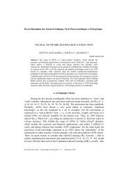
Fisher’s linear discriminants applied to the Iris data are shown in Figure 2.1. Six of the 

observations would be misclassified. 

Petal width 

0.0 0.5 1.0 1.5 2.0 2.5 3.0 

Setosa 

S 

S 

S 

S 

SS 

S 

S 

S 

S S 

S 

SSSS 

S 

S 

SS 

SS 

S 

S 

S 

S 

E 

Virginica 

A AA 

A A 

AAAA 

A A A A 

A A 

A 

AAAA 

A A 

AAAA 

A A 

AA 

A A 

AA EA 

A A 

A A A A 

A E 

E E E A 

E E 

EE 

E 

AA 

E E 

EE 

E A 

E EE 

E 

EEE 

EEE 

EE 

E E E 

EE 

E 

E 

E EE 

Versicolor 

0 2 4 6 8 

Petal length 

Fig. 2.1: Classification by linear discriminants: Iris data. 

2.2.2 Decision tree and Rule-based methods 

One class of classification procedures is based on recursive partitioning of the sample space. 

Space is divided into boxes, and at each stage in the procedure, each box is examined to 

see if it may be split into two boxes, the split usually being parallel to the coordinate axes. 

An example for the Iris data follows. 

If Petal Length 2.65 then Setosa. 

If Petal Length 4.95 then Virginica.


If 2.65 Petal Length 4.95 then : 

 

if Petal Width 1.65 then Versicolor; 

if Petal Width 1.65 then Virginica. 

The resulting partition is shown in Figure 2.2. Note that this classification rule has three 

mis-classifications. 

Petal width 

0.0 0.5 1.0 1.5 2.0 2.5 3.0 

Setosa 

S 

S 

S 

S 

SS 

S 

S 

S 

S S 

S 

SSSS 

S 

S 

SS 

SS 

S 

S 

S 

S 

E 

A AA 

A A 

AAAA 

A A A A 

A A 

A 

Virginica 

AAAA 

A A 

AAAA 

A A 

AA 

A A 

AA EA 

A A 

A A A A 

A E 

E E E A 

E E 

EE 

E 

AA 

E E 

EE 

E A 

E EE 

E 

EEE 

EEE 

EE 

E E E 

EE 

E 

E 

E EE 

Virginica 

Versicolor 

0 2 4 6 8 

Petal length 

Fig. 2.2: Classification by decision tree: Iris data. 

Weiss & Kapouleas (1989) give an alternative classification rule for the Iris data that is 

very directly related to Figure 2.2. Their rule can be obtained from Figure 2.2 by continuing 

the dotted line to the left, and can be stated thus: 

If Petal Length 2.65 then Setosa. 

If Petal Length 4.95 or Petal Width 1.65 then Virginica. 

Otherwise Versicolor. 

Notice that this rule, while equivalent to the rule illustrated in Figure 2.2, is stated more 

concisely, and this formulation may be preferred for this reason. Notice also that the rule is 

ambiguous if Petal Length 2.65 and Petal Width 1.65. The quoted rules may be made 

unambiguous by applying them in the given order, and they are then just a re-statement of 

the previous decision tree. The rule discussed here is an instance of a rule-based method: 

such methods have very close links with decision trees. 

2.2.3 k-Nearest-Neighbour 

We illustrate this technique on the Iris data. Suppose a new Iris is to be classified. The idea 

is that it is most likely to be near to observations from its own proper population. So we 

look at the five (say) nearest observations from all previously recorded Irises, and classify

Sec. 2.3] Variable selection 11 

the observation according to the most frequent class among its neighbours. In Figure 2.3, 

the new observation is marked by a , and the nearest observations lie within the circle 

centred on the . The apparent elliptical shape is due to the differing horizontal and vertical 

scales, but the proper scaling of the observations is a major difficulty of this method. 

This is illustrated in Figure 2.3 , where an observation centred at would be classified 

as Virginica since it has Virginica among its nearest neighbours. 

Petal width 

0.0 0.5 1.0 1.5 2.0 2.5 3.0 

S 

S 

S 

S 

SS 

S 

S 

S 

S S 

S 

SSSS 

S 

S 

SS 

SS 

S 

S 

S 

S 

E 

A AA 

A A 

AAAA 

A A A A 

A A 

A 

AAAA 

A A 

AAAA 

A A 

AA 

A A 

AA EA 

A A 

A A A A 

A E 

E E E A 

E E 

EE 

E 

AA 

E E 

EE 

E A 

E EE 

E 

EEE 

EEE 

EE 

E E E 

EE 

E 

E 

E EE 

Virginica 

0 2 4 6 8 

Petal length 

2.3 CHOICE OF VARIABLES 

Fig. 2.3: Classification by 5-Nearest-Neighbours: Iris data. 

As we have just pointed out in relation to k-nearest neighbour, it may be necessary to 

reduce the weight attached to some variables by suitable scaling. At one extreme, we might 

remove some variables altogether if they do not contribute usefully to the discrimination, 

although this is not always easy to decide. There are established procedures (for example, 

forward stepwise selection) for removing unnecessary variables in linear discriminants, 

but, for large datasets, the performance of linear discriminants is not seriously affected by 

including such unnecessary variables. In contrast, the presence of irrelevant variables is 

always a problem with k-nearest neighbour, regardless of dataset size. 

2.3.1 Transformations and combinations of variables 

Often problems can be simplified by a judicious transformation of variables. With statistical 

procedures, the aim is usually to transform the attributes so that their marginal density is 

approximately normal, usually by applying a monotonic transformation of the power law 

type. Monotonic transformations do not affect the Machine Learning methods, but they can 

benefit by combining variables, for example by taking ratios or differences of key variables. 

Background knowledge of the problem is of help in determining what transformation or


combination to use. For example, in the Iris data, the product of the variables Petal Length 

and Petal Width gives a single attribute which has the dimensions of area, and might be 

labelled as Petal Area. It so happens that a decision rule based on the single variable Petal 

Area is a good classifier with only four errors: 

If Petal Area 2.0 then Setosa. 

If 2.0 Petal Area 7.4 then Virginica. 

If Petal Area 7.4 then Virginica. 

This tree, while it has one more error than the decision tree quoted earlier, might be preferred 

on the grounds of conceptual simplicity as it involves only one “concept”, namely Petal 

Area. Also, one less arbitrary constant need be remembered (i.e. there is one less node or 

cut-point in the decision trees). 

2.4 CLASSIFICATION OF CLASSIFICATION PROCEDURES 

The above three procedures (linear discrimination, decision-tree and rule-based, k-nearest 

neighbour) are prototypes for three types of classification procedure. Not surprisingly, 

they have been refined and extended, but they still represent the major strands in current 

classification practice and research. The 23 procedures investigated in this book can be 

directly linked to one or other of the above. However, within this book the methods have 

been grouped around the more traditional headings of classical statistics, modern statistical 

techniques, Machine Learning and neural networks. Chapters 3 – 6, respectively, are 

devoted to each of these. For some methods, the classification is rather abitrary. 

2.4.1 Extensions to linear discrimination 

We can include in this group those procedures that start from linear combinations of 

the measurements, even if these combinations are subsequently subjected to some nonlinear 

transformation. There are 7 procedures of this type: Linear discriminants; logistic 

discriminants; quadratic discriminants; multi-layer perceptron (backprop and cascade); 

DIPOL92; and projection pursuit. Note that this group consists of statistical and neural 

network (specifically multilayer perceptron) methods only. 

2.4.2 Decision trees and Rule-based methods 

This is the most numerous group in the book with 9 procedures: NewID; §£¨¤© ; Cal5; CN2; 

C4.5; CART; IndCART; Bayes Tree; and ITrule (see Chapter 5). 

2.4.3 Density estimates 

This group is a little less homogeneous, but the 7 members have this in common: the 

procedure is intimately linked with the estimation of the local probability density at each 

point in sample space. The density estimate group contains: k-nearest neighbour; radial 

basis functions; Naive Bayes; Polytrees; Kohonen self-organising net; LVQ; and the kernel 

density method. This group also contains only statistical and neural net methods. 

2.5 A GENERAL STRUCTURE FOR CLASSIFICATION PROBLEMS 

There are three essential components to a classification problem. 

1. The relative frequency with which the classes occur in the population of interest, 

expressed formally as the prior probability distribution.

! 

Sec. 2.5] Costs of misclassification 13 

2. An implicit or explicit criterion for separating the classes: we may think of an underlying 

input/output relation that uses observed attributes to distinguish a random 

individual from each class. 

3. The cost associated with making a wrong classification. 

Most techniques implicitly confound components and, for example, produce a classification 

rule that is derived conditional on a particular prior distribution and cannot easily be 

adapted to a change in class frequency. However, in theory each of these components may 

be individually studied and then the results formally combined into a classification rule. 

We shall describe this development below. 

2.5.1 Prior probabilities and the Default rule 

We need to introduce some notation. Let the classes be denoted §!#"%$'&)(" * + "-, , and let 

the prior probability . ! for the class § ! be: 

.!/&10324§!65 

It is always possible to use the no-data rule: classify any new observation as class §£7 , 

irrespective of the attributes of the example. This no-data or default rule may even be 

adopted in practice if the cost of gathering the data is too high. Thus, banks may give 

credit to all their established customers for the sake of good customer relations: here the 

cost of gathering the data is the risk of losing customers. The default rule relies only on 

knowledge of the prior probabilities, and clearly the decision rule that has the greatest 

chance of success is to allocate every new observation to the most frequent class. However, 

if some classification errors are more serious than others we adopt the minimum risk (least 

expected cost) rule, and the class 8 is that with the least expected cost (see below). 

2.5.2 Separating classes 

Suppose we are able to observe data ¥ on an individual, and that we know the probability 

distribution of ¥ within each class §9! to be :;2 ¥=< §!>5 . Then for any two classes §9!?"@§BA the 

likelihood ratio :;2 ¥C< §9!>5%D:;2 ¥=< §EA*5 provides the theoretical optimal form for discriminating 

the classes on the basis of data ¥ . The majority of techniques featured in this book can be 

thought of as implicitly or explicitly deriving an approximate form for this likelihood ratio. 

2.5.3 Misclassification costs 

Suppose the cost of misclassifying a class § ! object as class § A is F*24$-"6GH5 . Decisions should 

be based on the principle that the total cost of misclassifications should be minimised: for 

a new observation this means minimising the expected cost of misclassification. 

Let us first consider the expected cost of applying the default decision rule: allocate 

all new observations to the class §£I , using suffix J as label for the decision class. When 

decision § I is made for all new examples, a cost of FK24$-"LJM5 is incurred for class § ! examples 

and these occur with probability . ! . So the expected cost ¨ I of making decision § I is: 

I &ON . ! F*24$-"-JP5 

¨ 

The Bayes minimum cost rule chooses that class that has the lowest expected cost. To 

see the relation between the minimum error and minimum cost rules, suppose the cost of

N 

! 

! 

A 


misclassifications to be the same for all errors and zero when a class is correctly identified, 

i.e. suppose F*2Q$L"6GH5R&SF that $UT &VG for FK24$-"WG5X& and $Y&ZG for . 

Then the expected cost is 

. ! &SFK2L( . I 5 

and the minimum cost rule is to allocate to the class with the greatest prior probability. 

Misclassification costs are very difficult to obtain in practice. Even in situations where 

it is very clear that there are very great inequalities in the sizes of the possible penalties 

or rewards for making the wrong or right decision, it is often very difficult to quantify 

them. Typically they may vary from individual to individual, as in the case of applications 

for credit of varying amounts in widely differing circumstances. In one dataset we have 

assumed the misclassification costs to be the same for all individuals. (In practice, creditgranting 

companies must assess the potential costs for each applicant, and in this case the 

classification algorithm usually delivers an assessment of probabilities, and the decision is 

left to the human operator.) 

! F*24$-"-JP5[& N . 

] I !@\ 

! F^&SF N . 

] I !6\ 

¨ I & 

2.6 BAYES RULE GIVEN DATA ¥ 

We can now see how the three components introduced above may be combined into a 

classification procedure. 

When we are given information ¥ about an individual, the situation is, in principle, 

unchanged from the no-data situation. The difference is that all probabilities must now 

be interpreted as conditional on the data ¥ . Again, the decision rule with least probability 

of error is to allocate to the class with the highest probability of occurrence, but now the 

relevant probability is the conditional probability 0_2Q§ ! < ¥ 5 of class § ! given the data ¥ : 

< 5/& Prob(class§9! given ¥ 5 

0_2Q§9! ¥ 

If we wish to use a minimum cost rule, we must first calculate the expected costs of the 

various decisions conditional on the given information . 

Now, when ¥ I decision is made for examples with attributes , a cost of F*2Q$L"-JM5 

§ 

is incurred for ¥ ! class examples and these occur with 0324§ ! < ¥ 5 probability . As the 

§ 

! < ¥ 5 probabilities depend on , so too will the decision rule. So too will the expected 

0_2Q§ ¥ 

I 2 ¥ 5 cost of making § I decision : 

¨ 

I 2 ¥ 5R&ON 0_2Q§ ! < ¥ 5%F*24$-"LJM5 

¨ 

In the special case of equal misclassification costs, the minimum cost rule is to allocate to 

the class with the greatest posterior probability. 

When Bayes theorem is used to calculate the conditional 0324§9! < ¥ 5 probabilities for the 

classes, we refer to them as the posterior probabilities of the classes. Then the posterior 

0324§! < ¥ 5 probabilities are calculated from a knowledge of the prior .! probabilities and the 

conditional :`2 ¥C< §!>5 probabilities of the data for each §! class . Thus, for §9! class suppose 

that the probability of observing data is :;2 ¥C< § ! 5 . Bayes theorem gives the posterior 

probability ¥ ! < ¥ 5 for class § ! as: 

0324§ 

0_2Q§ ! < ¥ 5/&a. ! :;2 ¥C< § ! 5%D N 

. A :;2 ¥=< § A 5

N 

N 

! 

! 

 

A 

Sec. 2.6] Bayes’ rule 15 

The divisor is common to all classes, so we may use the fact that 0_2Q§ ! < ¥ 5 is proportional 

to . ! :;2 ¥=< § ! 5 . The class § I with minimum expected cost (minimum risk) is therefore that 

for which 

! F*24$-"-JP5%:;2 ¥C< § ! 5 . 

is a minimum. 

Assuming now that the attributes have continuous distributions, the probabilities above 

become probability densities. Suppose that observations drawn from § ! population have 

probability density b ! 2 ¥ 5'&cb32 ¥;< § ! 5 function and that the prior probability that an observation 

belongs to §9! class .d! is . Then Bayes’ theorem computes the probability that an 

observation belongs to class §! as 

¥ 

! ¥ 5/&a. ! b ! 2 ¥ 5@D N . A b A 2 ¥ 5 

0_2Q§ < 

A classification rule then assigns to the §¡I class with maximal a posteriori probability 

given : 

¥ ¥ 

I < ¥ 5C& max 

! 0_2Q§ ! < ¥ 5 

0_2Q§ 

As before, the §¡I class with minimum expected cost (minimum risk) is that for which 

! F*24$-"-JP5%b ! 2 ¥ 5 . 

is a minimum. 

Consider the problem of discriminating between just two § ! classes § A and . Then 

assuming as before F*24$-"@$W5'&eF*2fG"6GH5g& that , we should allocate to $ class if 

A F*24$-"WG5@b A 2 ¥ 5'h. ! F*2iG"@$W5@b ! 2 ¥ 5 

. 

or equivalently 

F*2Q$L"6G5 

2 ¥ 5 . ! F*2fG"%$>5 

b A 

which shows the pivotal role of the likelihood ratio, which must be greater than the ratio of 

prior probabilities times the relative costs of the errors. We note the symmetry in the above 

expression: changes in costs can be compensated in changes in prior to keep constant the 

threshold that defines the classification rule - this facility is exploited in some techniques, 

although for more than two groups this property only exists under restrictive assumptions 

(see Breiman et al., page 112). 

b ! 2 ¥ 5 

. A 

2.6.1 Bayes rule in statistics 

Rather than deriving0_2Q§9! 

< ¥ 5 via Bayes theorem, we could also use the empirical frequency 

version of Bayes rule, which, in practice, would require prohibitivelylarge amounts of data. 

However, in principle, the procedure is to gather together all examples in the training set 

that have the same attributes (exactly) as the given example, and to find class proportions 

0324§ ! < ¥ 5 among these examples. The minimum error rule is to allocate to the class § I with 

highest posterior probability. 

Unless the number of attributes is very small and the training dataset very large, it will be 

necessary to use approximations to estimate the posterior class probabilities. For example,


one way of finding an approximate Bayes rule would be to use not just examples with 

attributes matching exactly those of the given example, but to use examples that were near 

the given example in some sense. The minimum error decision rule would be to allocate 

to the most frequent class among these matching examples. Partitioning algorithms, and 

decision trees in particular, divide up attribute space into regions of self-similarity: all 

data within a given box are treated as similar, and posterior class probabilities are constant 

within the box. 

Decision rules based on Bayes rules are optimal - no other rule has lower expected 

error rate, or lower expected misclassification costs. Although unattainable in practice, 

they provide the logical basis for all statistical algorithms. They are unattainable because 

they assume complete information is known about the statistical distributions in each class. 

Statistical procedures try to supply the missing distributional information in a variety of 

ways, but there are two main lines: parametric and non-parametric. Parametric methods 

make assumptions about the nature of the distributions (commonly it is assumed that the 

distributions are Gaussian), and the problem is reduced to estimating the parameters of 

the distributions (means and variances in the case of Gaussians). Non-parametric methods 

make no assumptions about the specific distributions involved, and are therefore described, 

perhaps more accurately, as distribution-free. 

2.7 REFERENCE TEXTS 

There are several good textbooks that we can recommend. Weiss & Kulikowski (1991) 

give an overall view of classification methods in a text that is probably the most accessible 

to the Machine Learning community. Hand (1981), Lachenbruch & Mickey (1975) and 

Kendall et al. (1983) give the statistical approach. Breiman et al. (1984) describe CART, 

which is a partitioning algorithm developed by statisticians, and Silverman (1986) discusses 

density estimation methods. For neural net approaches, the book by Hertz et al. (1991) is 

probably the most comprehensive and reliable. Two excellent texts on pattern recognition 

are those of Fukunaga (1990) , who gives a thorough treatment of classification problems, 

and Devijver & Kittler (1982) who concentrate on the k-nearest neighbour approach. 

A thorough treatment of statistical procedures is given in McLachlan (1992), who also 

mentions the more important alternative approaches. A recent text dealing with pattern 

recognition from a variety of perspectives is Schalkoff (1992).

3 

Classical Statistical Methods 

J. M. O. Mitchell 

University of Strathclyde 


This chapter provides an introduction to the classical statistical discrimination techniques 

and is intended for the non-statistical reader. It begins with Fisher’s linear discriminant, 

which requires no probability assumptions,and then introduces methods basedon maximum 

likelihood. These are linear discriminant, quadratic discriminant and logistic discriminant. 

Next there is a brief section on Bayes’ rules, which indicates how each of the methods 

can be adapted to deal with unequal prior probabilities and unequal misclassification costs. 

Finally there is an illustrative example showing the result of applying all three methods to 

a two class and two attribute problem. For full details of the statistical theory involved the 

reader should consult a statistical text book, for example (Anderson, 1958). 

The training set will consist of examples drawn , from known classes. , (Often will 

be 2.) The values 0 of numerically-valued attributes will be known for each j of examples, 

and these form the attribute kl&m2 ¥ 

" ¥ 

© " ** " ¥n 5 vector . It should be noted that these 

methods require numerical attribute vectors, and also require that none of the values is 

missing. Where an attribute is categorical with two values, an indicator is used, i.e. an 

attribute which takes the value 1 for one category, and 0 for the other. Where there are 

more than two categorical values, indicators are normally set up for each of the values. 

However there is then redundancy among these new attributes and the usual procedure is 

to drop one of them. In this way a single categorical attribute G with values is replaced by 

( attributes whose values are 0 or 1. Where the attribute values are ordered, it may be 

G 

acceptable to use a single numerical-valued attribute. Care has to be taken that the numbers 

used reflect the spacing of the categories in an appropriate fashion. 

3.2 LINEAR DISCRIMINANTS 

There are two quite different justifications for using Fisher’s linear discriminant rule: the 

first, as given by Fisher (1936), is that it maximises the separation between the classes in 



x 

r 2 o 

r 2?o 

r 2 o 

2 

2 o k r 5 © 

2 o k r 5 © 

5 

18 Classical statistical methods [Ch. 3 

a least-squares sense; the second is by Maximum Likelihood (see Section 3.2.3). We will 

give a brief outline of these approaches. For a proof that they arrive at the same solution, 

we refer the reader to McLachlan (1992). 

3.2.1 Linear discriminants by least squares 

Fisher’s linear discriminant (Fisher, 1936) is an empirical method for classification based 

purely on attribute vectors. A hyperplane (line in two dimensions,plane in three dimensions, 

etc.) in 0 the -dimensional attribute space is chosen to separate the known classes as well 

as possible. Points are classified according to the side of the hyperplane that they fall on. 

For example, see Figure 3.1, which illustrates discrimination between two “digits”, with 

the continuous line as the discriminating hyperplane between the two populations. 

This procedure is also equivalent to a t-test or F-test for a significant difference between 

the mean discriminants for the two samples, the t-statistic or F-statistic being constructed 

to have the largest possible value. 

More precisely, in the case of two classes, o k let o k 

, o k © 

, be respectively the means of 

the attribute vectors overall and for the two classes. Suppose that we are given a set of 

p " q q "Lp n 

coefficients and let us call the particular linear combination of attributes 

2Qks5E&eN p A ¥ A r 

the discriminant between the classes. We wish the discriminants for the two classes to 

differ as much as possible, and one measure for this is the difference 2?o k 5 r 2to k © 5 r 

between the mean discriminants for the two classes divided by the standard deviation of 

the discriminants, u?v say, giving the following measure of discrimination: 

v u 

This measure of discrimination is related to an estimate of misclassification error based on 

the assumption of a multivariate normal distribution for 2Qks5 (note that this is a weaker 

assumption than saying that x has a normal distribution). For the sake of argument, we 

set the dividing line between the two classes at the midpoint between the two class means. 

r 

Then we may estimate the probability of misclassification for one class as the probability 

that the normal random variable 24ks5 for that class is on the wrong side of the dividing 

line, i.e. the wrong side of 

r 

k 5 

 

and this is easily seen to be 

5w r 2?o k © 5 k 

u v 

where we assume, without loss of generality, that 2?o k 5 r 2?o k © 5 is negative. If the classes 

are not of equal sizes, or if, as is very frequently the case, the variance of r 

r is not the 24ks5 

same for the two classes, the dividing line is best drawn at some point other than the 

midpoint. 

Rather than use the simple measure quoted above, it is more convenient algebraically 

to use an equivalent measure defined in terms of sums of squared deviations, as in analysis 

of variance. The sum of squares of 24ks5 within class § ! is 

r 

k 5

ƒ 

& 

 

† 

ƒ 

Sec. 3.2] Linear discrimination 19 

2 r 24ks5 r 2?o ky!L5@5 © " 

N 

the sum being over the examples in § ! class . The pooled sum of squares within z classes, 

say, is the sum of these quantities for the two classes (this is the quantity that would give 

us a standard u v deviation ). The total sum of squares of 24ks5 is {|2 r 24ks5 r 2 o k=5%5@©9&~} say, 

r 

where this last sum is now over both classes. By subtraction, the pooled sum of squares 

between classes } z is , and this last quantity is proportional 2 r 2 o k 5 r 2 o k © 5%5@© to . 

In terms of the F-test for the significance of the difference 2?o k 5 r 2to k © 5 , we would 

r 

calculate the F-statistic 

zP5@Dd( 2f} 

5 zMDM2W€ 

Clearly maximising the F-ratio statistic is equivalent to maximising the }LDHz ratio , so the 

p*A coefficients G¢&‚(" * + "40 , may be chosen to maximise the }LDz ratio . This maximisation 

problem may be solved analytically, giving an explicit solution for the p ! coefficients . 

There is however an arbitrary multiplicative constant in the solution, and the usual practice 

is to normalise p A the in some way so that the solution is uniquely determined. Often one 

coefficient is taken to be unity (so avoiding a multiplication). However the detail of this 

need not concern us here. 

To justify the “least squares” of the title for this section, note that we may choose the 

arbitrary multiplicative constant so that the separation 2 o k 5 r 2 o k © 5 between the class 

mean discriminants is equal to some predetermined value (say unity). Maximising the F- 

ratio is now equivalent to minimising the total sum of squares r . Put this way, the problem 

z 

is identical to a regression of class (treated numerically) on the attributes, the dependent 

variable class being zero for one class and unity for the other. 

The main point about this method is that it is a linear function of the attributes that is 

used to carry out the classification. This often works well, but it is easy to see that it may 

work badly if a linear separator is not appropriate. This could happen for example if the 

data for one class formed a tight cluster and the the values for the other class were widely 

spread around it. However the coordinate system used is of no importance. Equivalent 

results will be obtained after any linear transformation of the coordinates. 

A practical complication is that for the algorithm to work the pooled sample covariance 

matrix must be invertible. The covariance matrix for a dataset j ! with examples from 

§ ! class , is 

where is jy!ˆ‰0 the matrix of attribute values, o k and is 0 the -dimensional row-vector 

of attribute means. The pooled covariance matrix is { 24jy! (+5 !LDM24j ,5 where the 

… 

summation is over all the classes, and the ƒ , divisor is chosen to make the pooled 

j 

covariance matrix unbiased. For invertibility the attributes must be linearly independent, 

which means that no attribute may be an exact linear combination of other attributes. In 

order to achieve this, some attributes may have to be dropped. Moreover no attribute can 

be constant within each class. Of course an attribute which is constant within each class 

but not overall may be an excellent discriminator and is likely to be utilised in decision tree 

algorithms. However it will cause the linear discriminant algorithm to fail. This situation 

can be treated by adding a small positive constant to the corresponding diagonal element of 

( 

(M…‡†„… jy! 

o ¥ " 

!„& 

ko

† 


the pooled covariance matrix, or by adding random noise to the attribute before applying 

the algorithm. 

In order to deal with the case of more than two classes Fisher (1938) suggested the use 

of canonical variates. First a linear combination of the attributes is chosen to minimise 

the ratio of the pooled within class sum of squares to the total sum of squares. Then 

further linear functions are found to improve the discrimination. 

(The coefficients in 

these functions are the eigenvectors corresponding to the non-zero eigenvalues of a certain 

matrix.) In general there will be min2>, ("40y5 canonical variates. It may turn out that only 

a few of the canonical variates are important. Then an observation can be assigned to the 

class whose centroid is closest in the subspace defined by these variates. It is especially 

useful when the class means are ordered, or lie along a simple curve in attribute-space. In 

the simplest case, the class means lie along a straight line. This is the case for the head 

injury data (see Section 9.4.1), for example, and, in general, arises when the classes are 

ordered in some sense. In this book, this procedure was not used as a classifier, but rather 

in a qualitative sense to give some measure of reduced dimensionality in attribute space. 

Since this technique can also be used as a basis for explaining differences in mean vectors 

as in Analysis of Variance, the procedure may be called manova, standing for Multivariate 

Analysis of Variance. 

3.2.2 Special case of two classes 

The linear discriminant procedure is particularly easy to program when there are just two 

classes, for then the Fisher discriminant problem is equivalent to a multiple regression 

problem, with the attributes being used to predict the class value which is treated as 

a numerical-valued variable. 

The class values are converted to numerical values: for 

example, class § 

is given the value 0 and class § © 

is given the value 1. A standard 

multiple regression package is then used to predict the class value. If the two classes are 

equiprobable, the discriminating hyperplane bisects the line joining the class centroids. 

Otherwise, the discriminating hyperplane is closer to the less frequent class. The formulae 

are most easily derived by considering the multiple regression predictor as a single attribute 

that is to be used as a one-dimensional discriminant, and then applying the formulae of 

the following section. The procedure is simple, but the details cannot be expressed simply. 

See Ripley (1993) for the explicit connection between discrimination and regression. 

3.2.3 Linear discriminants by maximum likelihood 

The justification of the other statistical algorithms depends on the consideration of probability 

distributions, and the linear discriminant procedure itself has a justification of this 

kind. It is assumed that the attribute vectors for examples of class § ! are independent 

and follow a certain probability distribution with probability density function (pdf) b ! . A 

new point with attribute vector x is then assigned to that class for which the probability 

density function b ! 2 x5 is greatest. This is a maximum likelihood method. A frequently 

made assumption is that the distributions are normal (or Gaussian) with different means 

but the same covariance matrix. The probability density function of the normal distribution 

is 

Š 

( 

.s‹ < exp 2 < 

( 

 

24k Œ 5 

‹ Ž 24k XŒ 5%5?" (3.1)

k 

† 

log . ! k 

 

† 

( 

Œ 

 

( 

 

( 

Œ 

 

† 

 

Sec. 3.3] Linear discrimination 21 

where Œ is a 0 -dimensional vector denoting the (theoretical) mean for a class and ‹ , 

the (theoretical) covariance matrix, is a 0R‰0 (necessarily positive definite) matrix. The 

(sample) covariance matrix that we saw earlier is the sample analogue of this covariance 

matrix, which is best thought of as a set of coefficients in the pdf or a set of parameters for 

the distribution. This means that the points for the class are distributed in a cluster centered 

at Œ of ellipsoidal shape described by ‹ . Each cluster has the same orientation and spread 

though their means will of course be different. (It should be noted that there is in theory 

no absolute boundary for the clusters but the contours for the probability density function 

have ellipsoidal shape. In practice occurrences of examples outside a certain ellipsoid 

will be extremely rare.) In this case it can be shown that the boundary separating two 

classes, defined by equality of the two pdfs, is indeed a hyperplane and it passes through 

the mid-point of the two centres. Its equation is 

Ž 2 Œ ^Œ 

© 5 2 Œ 

 

Œ 

© 5 ‹ Ž 2 Œ ^Œ 

© 5'& " (3.2) 

‹ 

Œ ! where denotes the population mean for §9! class . However in classification the exact 

distribution is usually not known, and it becomes necessary to estimate the parameters for 

the distributions. With two classes, if the sample means are substituted Œ ! for and the 

pooled sample covariance matrix ‹ for , then Fisher’s linear discriminant is obtained. With 

more than two classes, this method does not in general give the same results as Fisher’s 

discriminant. 

3.2.4 More than two classes 

When there are more than two classes, it is no longer possible to use a single linear 

discriminant score to separate the classes. The simplest procedure is to calculate a linear 

discriminant for each class, this discriminant being just the logarithm of the estimated 

probability density function for the appropriate class, with constant terms dropped. Sample 

values are substituted for population values where these are unknown (this gives the “plugin” 

estimates). Where the prior class proportions are unknown, they would be estimated 

by the relative frequencies in the training set. Similarly, the sample means and pooled 

covariance matrix are substituted for the population means and covariance matrix. 

Suppose the prior probability of class §9! is .! , and that bt!L2 ¥ 5 is the probability density 

of ¥ in class §9! , and is the normal density given in Equation (3.1). The joint probability 

of observing class §! and attribute ¥ is .d!6bt!-2 ¥ 5 and the logarithm of the probability of 

observing class §! and attribute k is 

! ‹ Ž Œ ! 

† 

to within an additive constant. So the coefficients 

‹ Ž Œ ! 

! are given by the coefficients of x 

&S‹ Ž Œ ! ! 

and the additive ‘ ! constant by 

log .! 

† 

! ‹ Ž Œ ! 

‘3!’& 

though these can be simplified by subtracting the coefficients for the last class. 

The above formulae are stated in terms of the (generally unknown) population parameters 

Œ , i . ! and . To obtain the corresponding “plug-in” formulae, substitute the 

‹ 

corresponding sample estimators: for ‹ ; o k ! for Œ i; and 0 ! for . ! , where 0 ! is the sample 

proportion of class ƒ ! examples. §

log . ! b ! 2 ¥ 5'& log2Q. ! 5 

( 

 

( 

 

† 

† 


3.3 QUADRATIC DISCRIMINANT 

Quadratic discrimination is similar to linear discrimination, but the boundary between two 

discrimination regions is now allowed to be a quadratic surface. When the assumption 

of equal covariance matrices is dropped, then in the maximum likelihood argument with 

normal distributions a quadratic surface (for example, ellipsoid, hyperboloid, etc.) 

obtained. This type of discrimination can deal with classifications where the set of attribute 

values for one class to some extent surrounds that for another. Clarke et al. (1979) find 

that the quadratic discriminant procedure is robust to small departures from normality 

and that heavy kurtosis (heavier tailed distributions than gaussian) does not substantially 

reduce accuracy. However, the number of parameters to be estimated becomes ,-0_2“0” ‰(*5@D , 

and the difference between the variances would need to be considerable to justify the use 

of this method, especially for small or moderate sized datasets (Marks & Dunn, 1974). 

Occasionally, differences in the covariances are of scale only and some simplification may 

occur (Kendall et al., 1983) . Linear discriminant is thought to be still effective if the 

departure from equality of covariances is small (Gilbert, 1969). Some aspects of quadratic 

dependence may be included in the linear or logistic form (see below) by adjoining new 

attributes that are quadratic functions of the given attributes. 

3.3.1 Quadratic discriminant - programming details 

The quadratic discriminant function is most simply defined as the logarithm of the appropriate 

probability density function, so that one quadratic discriminant is calculated for 

each class. The procedure used is to take the logarithm of the probability density function 

and to substitute the sample means and covariance matrices in place of the population 

values, giving the so-called “plug-in” estimates. Taking the logarithm of Equation (3.1), 

and allowing for differing prior class probabilities . ! , we obtain 

is 

Ž ! 24k ^Œ ! 5 ‹ 

as the quadratic discriminant for § ! class . Here it is understood that the $ suffix refers to 

the sample of values from § ! class . 

In classification, the quadratic discriminant is calculated for each class and the class 

with the largest discriminant is chosen. To find the a posteriori class probabilities explicitly, 

the exponential is taken of the discriminant and the resulting quantities normalised to sum 

to unity (see Section 2.6). Thus the posterior class :`24§ ! < ks5 probabilities are given by 

log2 

< ‹ ! < 5 

24k ^Œ ! 5 

apart from a normalising factor. 

If there is a cost matrix, then, no matter the number of classes, the simplest procedure is 

to calculate the class probabilities :;24§ ! < ks5 and associated expected costs explicitly, using 

the formulae of Section 2.6. The most frequent problem with quadratic discriminants is 

caused when some attribute has zero variance in one class, for then the covariance matrix 

cannot be inverted. One way of avoiding this problem is to add a small positive constant 

term to the diagonal terms in the covariance matrix (this corresponds to adding random 

noise to the attributes). Another way, adopted in our own implementation, is to use some 

combination of the class covariance and the pooled covariance. 

( 

 

( 

 

:;24§ ! < ks5/& exp• log24. ! 5 

log2 

< ‹ ! < 5 

2Qk ^Œ ! 5 

Ž ! 24k Œ ! 5>– ‹

ƒ 

Sec. 3.3] Quadratic discrimination 23 

Once again, the above formulae are stated in terms of the unknown population pa- 

‹ ! rameters Œ , i . ! and . To obtain the corresponding “plug-in” formulae, substitute the 

corresponding sample estimators: ! for ‹ ! ; o k ! for Œ i; and 0 ! for . ! , where0 ! is the sample 

proportion of class ƒ ! examples. § 

Many statistical packages allow for quadratic discrimination (for example, MINITAB 

has an option for quadratic discrimination, SAS also does quadratic discrimination). 

3.3.2 Regularisation and smoothed estimates 

The main problem with quadratic discriminants is the large number of parameters that 

need to be estimated and the resulting large variance of the estimated discriminants. A 

related problem is the presence of zero or near zero eigenvalues of the sample covariance 

matrices. Attempts to alleviate this problem are known as regularisation methods, and 

the most practically useful of these was put forward by Friedman (1989), who proposed 

a compromise between linear and quadratic discriminants via a two-parameter family of 

estimates. One parameter controls the smoothing of the class covariance matrix estimates. 

The smoothed estimate of the class $ covariance matrix is 

! 5 ! — ! 

ƒ 

2L( — 

! where is the $ class sample covariance matrix and is the pooled covariance matrix. 

When ƒ ƒ is zero, there is no smoothing and the estimated class $ covariance matrix is just 

— ! 

the i’th sample covariance ! matrix . When — ! the are unity, all classes have the same 

covariance matrix, namely the pooled covariance matrix . Friedman (1989) makes the 

value of ƒ ƒ smaller for classes with larger numbers. For the i’th sample with j ! observations: 

! — 

! & — 2W€ ,5%D˜ — 2>€ ,5‡ 2-( — 5#24j ! (+5%š 

— 

€›&lj œj © 

q ^js where . 

The other ž parameter is a (small) constant term that is added to the diagonals of the 

covariance matrices: this is done to make the covariance matrix non-singular, and also has 

the effect of smoothing out the covariance matrices. As we have already mentioned in 

connection with linear discriminants, any singularity of the covariance matrix will cause 

problems, and as there is now one covariance matrix for each class the likelihood of such 

a problem is much greater, especially for the classes with small sample sizes. 

This two-parameter family of procedures is described by Friedman (1989) as “regularised 

discriminant analysis”. Various simple procedures are included as special cases: 

ordinary linear (— &Ÿ("-ž‰& discriminants ); quadratic (— & "Lž[& discriminants ); and 

the — & ("-žw& ( values correspond to a minimum Euclidean distance rule. 

This type of regularisation has been incorporated in the Strathclyde version of Quadisc. 

Very little extra programming effort is required. However, it is up to the user, by trial and 

error, to choose the values — of ž and . Friedman (1989) gives various shortcut methods for 

reducing the amount of computation. 

3.3.3 Choice of regularisation parameters 

The default values of — & and ž[& were adopted for the majority of StatLog datasets, 

the philosophy being to keep the procedure “pure” quadratic. 

The exceptions were those cases where a covariance matrix was not invertible. Nondefault 

values were used for the head injury dataset (ž =0.05) and the DNA dataset (— =0.3

log b 24ks5 

. . b © 24ks5 © 

:;24§ 

:;24§ © 

¥ 

< ks5¤& 

< ks5¤& 

( 

exp2>‘‡ / ¡ ks5 (' 

ks5 ¦ < 

sampleª 

§%¨s« 


approx.). In practice, great improvements in the performance of quadratic discriminants 

may result from the use of regularisation, especially in the smaller datasets. 

3.4 LOGISTIC DISCRIMINANT 

Exactly as in Section 3.2, logistic regression operates by choosing a hyperplane to separate 

the classes as well as possible, but the criterion for a good separation is changed. Fisher’s 

linear discriminants optimises a quadratic cost function whereas in logistic discrimination 

it is a conditional likelihood that is maximised. However, in practice, there is often very 

little difference between the two, and the linear discriminants provide good starting values 

for the logistic. Logistic discrimination is identical, in theory, to linear discrimination for 

normal distributions with equal covariances, and also for independent binary attributes, so 

the greatest differences between the two are to be expected when we are far from these 

two cases, for example when the attributes have very non-normal distributions with very 

dissimilar covariances. 

The method is only partially parametric, as the actual pdfs for the classes are not 

modelled, but rather the ratios between them. 

Specifically, the logarithms of the prior odds . D. © 

times the ratios of the probability 

density functions for the classes are modelled as linear functions of the attributes. Thus, 

for two classes, 

C¡“k'" &l‘‡ 

‘ where and 0 the -dimensional vector are the parameters of the model that are to be 

estimated. The case of normal distributions with equal covariance is a special case of 

this, for which the parameters are functions of the prior probabilities, the class means and 

the common covariance matrix. However the model covers other cases too, such as that 

where the attributes are independent with values 0 or 1. One of the attractions is that the 

discriminant scale covers all real numbers. A large positive value indicates that § 

class is 

likely, while a large negative value indicates that § © 

class is likely. 

In practice the parameters are estimated by F?¢*jsJ$i}@$>¢*jspM£ maximum likelihood. The 

model implies that, given attribute values x, the conditional class probabilities for classes 

 

and § © 

take the forms: 

§ 

exp2>‘‰ 

¡ ks5 

(' exp2>‘‡ / ¡ ks5 

respectively. 

Given independent samples from the two classes, the conditional likelihood for the 

‘ parameters and is defined to be 

:;2Q§ 

:;24§ © 

< ks5 

and the parameter estimates are the values that maximise this likelihood. They are found by 

iterative methods, as proposed by Cox (1966) and Day & Kerridge (1967). Logistic models 

¦ 2>‘B"Q'5X& 

sampleª 

§%¨C©

¥ 

" q q "4 Ž 5/& ¦ 

2“ 

© 

sampleª 

§%¨ 

( 

ks5 ¦ < 

« 

sampleª 

§%¨ 

ks5 + * ¦ < 

sampleª 

§%¨s° 

< ks5 

Sec. 3.4] Logistic discrimination 25 

belong to the class of generalised linear models (GLMs), which generalise the use of linear 

regression models to deal with non-normal random variables, and in particular to deal with 

binomial variables. In this context, the binomial variable is an indicator variable that counts 

whether an example is class § 

or not. When there are more than two classes, one class is 

taken as a reference class, and there are , ( sets of parameters for the odds of each class 

relative to the reference class. To discuss this case, we abbreviate the notation for ‘w / ¡ k 

to the ¡ k simpler . For the remainder of this section, therefore, x is 2“0¢ ¬(+5 a -dimensional 

vector with leading term unity, and the leading term in corresponds to the ‘ constant . 

Again, the parameters are estimated by maximum conditional likelihood. Given at- 

, and the &a, 

conditional class probability § for take the forms: 

tribute values x, the conditional class probability for class § ! , where $T 

exp2“ ¡ 

! ks5 

:;24§ ! < ks5& 

A ks5 exp2qC¡ 

N 

] A 

-®¯¯® 

:;24§¡ < ks5& 

N 

] A 

-®¯¯® 

respectively. Given independent samples from , the classes, the conditional likelihood for 

the y! parameters is defined to be 

A ks5 exp2qC¡ 

:`24§ 

:;24§ © 

:;2Q§ 

Once again, the parameter estimates are the values that maximise this likelihood. 

In the basic form of the algorithm an example is assigned to the class for which the 

posterior is greatest if that is greater than 0, or to the reference class if all posteriors are 

negative. 

More complicated models can be accommodated by adding transformations of the 

given attributes, for example products of pairs of attributes. As mentioned in Section 

3.1, when categorical attributes ± ( with ) values occur, it will generally be necessary 

to convert them ± ( into binary attributes before using the algorithm, especially if the 

categories are not ordered. Anderson (1984) points out that it may be appropriate to 

include transformations or products of the attributes in the linear function, but for large 

datasets this may involve much computation. See McLachlan (1992) for useful hints. One 

way to increase complexity of model, without sacrificing intelligibility, is to add parameters 

in a hierarchical fashion, and there are then links with graphical models and Polytrees. 

3.4.1 Logistic discriminant - programming details 

Most statistics packages can deal with linear discriminant analysis for two classes. SYSTAT 

has, in addition, a version of logistic regression capable of handling problems with more 

than two classes. If a package has only binary logistic regression (i.e. can only deal with 

two classes), Begg & Gray (1984) suggest an approximate procedure whereby classes are 

all compared to a reference class by means of logistic regressions, and the results then 

combined. The approximation is fairly good in practice according to Begg & Gray (1984).


Many statistical packages (GLIM, Splus, Genstat) now include a generalised linear 

model (GLM) function, enabling logistic regression to be programmed easily, in two 

or three lines of code. The procedure is to define an indicator variable for § 

class 

occurrences. The indicator variable is then declared to be a “binomial” variable with the 

“logit” link function, and generalised regression performed on the attributes. We used the 

package Splus for this purpose. This is fine for two classes, and has the merit of requiring 

little extra programming effort. For more than two classes, the complexity of the problem 

increases substantially, and, although it is technically still possible to use GLM procedures, 

the programming effort is substantially greater and much less efficient. 

The maximum likelihood solution can be found via a Newton-Raphson iterative procedure, 

as it is quite easy to write down the necessary derivatives of the likelihood (or, 

equivalently, the log-likelihood). The simplest starting procedure is to set ! the coefficients 

to zero except for the leading coefficients (‘ ! ) which are set to the logarithms of the 

numbers in the various classes: i.e. ‘ ! & log j ! , where j ! is the number of class § ! 

examples. This ensures that the values ! of are those of the linear discriminant after the 

first iteration. Of course, an alternative would be to use the linear discriminant parameters 

as starting values. In subsequent iterations, the step size may occasionally have to be 

reduced, but usually the procedure converges in about 10 iterations. This is the procedure 

we adopted where possible. 

However, each iteration requires a separate calculation of the Hessian, and it is here 

that the bulk of the computational work is required. The Hessian is a square matrix with 

2W, (*5-2q0² e(+5 rows, and each term requires a summation over all the observations in the 

whole dataset (although some saving can by achieved using the symmetries of the Hessian). 

Thus there are of ,©W0y©+€ order computations required to find the Hessian matrix at each 

iteration. In the KL digits dataset (see Section 9.3.2), for example, , &³( , 0e& M , 

and €O&m´ , so the number of operations is of order ( µ in each iteration. In such 

cases, it is preferable to use a purely numerical search procedure, or, as we did when 

the Newton-Raphson procedure was too time-consuming, to use a method based on an 

approximate Hessian. The approximation uses the fact that the Hessian for the zero’th 

order iteration is simply a replicate of the design matrix (cf. covariance matrix) used by 

the linear discriminant rule. This zero-order Hessian is used for all iterations. In situations 

where there is little difference between the linear and logistic parameters, the approximation 

is very good and convergence is fairly fast (although a few more iterations are generally 

required). However, in the more interesting case that the linear and logistic parameters 

are very different, convergence using this procedure is very slow, and it may still be quite 

far from convergence after, say, 100 iterations. We generally stopped after 50 iterations: 

although the parameter values were generally not stable, the predicted classes for the data 

were reasonably stable, so the predictive power of the resulting rule may not be seriously 

affected. This aspect of logistic regression has not been explored. 

The final program used for the trials reported in this book was coded in Fortran, since 

the Splus procedure had prohibitive memory requirements. Availablility of the Fortran 

code can be found in Appendix B.

© . 

. 

" 

Sec. 3.6] Bayes’ rules 27 

3.5 BAYES’ RULES 

Methods based on likelihood ratios can be adapted to cover the case of unequal misclassification 

costs and/or unequal prior probabilities. Let the prior probabilities be 

! : $w)(" * + "L,š , and let F*2Q$L"6G5 denote the cost incurred by classifying an example 

˜H. 

of § ! Class into § A class . 

As in Section 2.6, the minimum expected cost solution is to assign the data x to class 

I chosen to minimise { ! . ! F*24$-"-JP5%b_2Qk < § ! 5 . In the case of two classes the hyperplane in 

§ 

linear discrimination has the equation 

( 

F*2 "+(*5 

F*2L(" 5¸ 

 

the right hand side replacing 0 that we had in Equation (3.2). 

When there are more than two classes, the simplest procedure is to calculate the 

class :`24§9! < ks5 probabilities and associated expected costs explicitly, using the formulae of 

Section 2.6. 

k_¡f‹ Ž 2 Œ 

Œ 

2 Œ 

XŒ 

© 5 

 

Œ 

© 5W¡Q2 Œ 

© 5C& log· 

3.6 EXAMPLE 

As illustration of the differences between the linear, quadratic and logistic discriminants, 

we consider a subset of the Karhunen-Loeve version of the digits data later studied in this 

book. For simplicity, we consider only the digits ‘1’ and ‘2’, and to differentiate between 

them we use only the first two attributes (40 are available, so this is a substantial reduction 

in potential information). The full sample of 900 points for each digit was used to estimate 

the parameters of the discriminants, although only a subset of 200 points for each digit is 

plotted in Figure 3.1 as much of the detail is obscured when the full set is plotted. 

3.6.1 Linear discriminant 

Also shown in Figure 3.1 are the sample centres of gravity (marked by a cross). Because 

there are equal numbers in the samples, the linear discriminant boundary (shown on the 

diagram by a full line) intersects the line joining the centres of gravity at its mid-point. Any 

new point is classified as a ‘1’ if it lies below the line i.e. is on the same side as the centre 

of the ‘1’s). In the diagram, there are 18 ‘2’s below the line, so they would be misclassified. 

3.6.2 Logistic discriminant 

The logistic discriminant procedure usually starts with the linear discriminant line and then 

adjusts the slope and intersect to maximise the conditional likelihood, arriving at the dashed 

line of the diagram. Essentially, the line is shifted towards the centre of the ‘1’s so as to 

reduce the number of misclassified ‘2’s. This gives 7 fewer misclassified ‘2’s (but 2 more 

misclassified ‘1’s) in the diagram. 

3.6.3 Quadratic discriminant 

The quadratic discriminant starts by constructing, for each sample, an ellipse centred on 

the centre of gravity of the points. In Figure 3.1 it is clear that the distributions are of 

different shape and spread, with the distribution of ‘2’s being roughly circular in shape 

and the ‘1’s being more elliptical. The line of equal likelihood is now itself an ellipse (in 

general a conic section) as shown in the Figure. All points within the ellipse are classified


as ‘1’s. Relative to the logistic boundary, i.e. in the region between the dashed line and the 

ellipse, the quadratic rule misclassifies an extra 7 ‘1’s (in the upper half of the diagram) but 

correctly classifies an extra 8 ‘2’s (in the lower half of the diagram). So the performance of 

the quadratic classifier is about the same as the logistic discriminant in this case, probably 

due to the skewness of the ‘1’ distribution. 

Linear, Logistic and Quadratic discriminants 

2nd KL-variate 

50 100 150 

1 

2 

2 

2 2 

2 

1 

2 

2 

2 2 

2 

2 

2 

2 2 

2 

2 

2 

2 

2 

2 

2 2 

2 2 2 

2 

2 

2 2 

2 

2 

2 2 

2 2 

2 

1 

2 

1 

2 

2 2 

2 

2 

2 

2 2 

2 

2 2 2 

1 1 2 

2 

2 

1 

2 

2 

2 

2 2 

2 22 

2 

2 

2 

1 2 1 

2 2 2 

1 

2 2 

22 

2 

2 

2 

2 

2 

2 

1 

2 2 

1 2 

2 

2 

2 2 

2 

2 2 2 

2 

2 

1 

1 

1 

2 

2 2 2 

2 2 

2 2 

2 

1 1 

1 1 

2 

2 

2 2 2 

1 1 

2 

2 2 

2 

1 

2 

2 

2 2 

2 

1 

1 1 1 

2 

1 

1 

2 

2 

1 

1 

2 

1 1 1 

2 

2 

2 2 

1 

1 1 2 

1 

1 

1 

1 

1 

2 

12 

1 

1 

11 

1 

1 

2 

1 

2 

1 

1 1 

1 

1 

1 

1 

1 

1 1 

1 1 1 1 

11 

1 1 

1 1 

2 

2 2 

1 1 

1 1 

1 

1 

1 1 1 

2 

11 

1 

1 

50 100 150 200 

1st KL-variate 

2 

Linear 

Logistic 

¹ 

Quadratic 

2 

Fig. 3.1: Decision boundaries for the three discriminants: quadratic (curved); linear (full line); and 

logistic (dashed line). The data are the first two Karhunen-Loeve components for the digits ‘1’ and 

‘2’.

4 

Modern Statistical Techniques 

R. Molina (1), N. Pérez de la Blanca (1) and C. C. Taylor (2) 

(1) University of Granada and (2) University of Leeds 


In the previous chapter we studied the classification problem, from the statistical point of 

view, assuming that the form of the underlying density functions (or their ratio) was known. 

However, in most real problems this assumption does not necessarily hold. In this chapter 

we examine distribution-free (often called nonparametric) classification procedures that 

can be used without assuming that the form of the underlying densities are known. 

Recall that ,M"%j'"40 denote the number of classes, of examples and attributes, respectively. 

Classes will be denoted by § "%§ © " * + "%§£ and attribute values for example $ 

(" " + * "%js5 will be denoted by the0 -dimensional vectorky!º&|2 ¥ 

!L" ¥ 

© !L" + * " ¥n !W5B’» . 

2Q$=& 

Elements » in will be k/&|2 ¥ 

" ¥ 

© " + * " ¥n 5 denoted . 

The Bayesian approach for allocating observations to classes has already been outlined 

in Section 2.6. It is clear that to apply the Bayesian approach to classification we have 

to b_2Qk < § A 5 estimate . A and 0_2Q§ A < ks5 or . Nonparametric methods to do this job will be 

discussed in this chapter. We begin in Section 4.2 with kernel density estimation; a close 

relative to this approach is the k-nearest neighbour (k-NN) which is outlined in Section 4.3. 

Bayesian methods which either allow for, or prohibit dependence between the variables 

are discussed in Sections 4.5 and 4.6. A final section deals with promising methods 

which have been developed recently, but, for various reasons, must be regarded as methods 

for the future. To a greater or lesser extent, these methods have been tried out in the 

project, but the results were disappointing. In some cases (ACE), this is due to limitations 

of size and memory as implemented in Splus. The pruned implementation of MARS in 

Splus (StatSci, 1991) also suffered in a similar way, but a standalone version which also 

does classification is expected shortly. We believe that these methods will have a place in 

classification practice, once some relatively minor technical problems have been resolved. 

As yet, however, we cannot recommend them on the basis of our empirical trials. 

Address for correspondence: Department of Computer Science and AI, Facultad de Ciencas, University of 

Granada, 18071 Granada, Spain

Ê 

¦ 

( 

j 

( 

j 

Â 

N 

Â 

 

 

( 

ÁMÂÇÆ|È 

¦ 

ky! k 

žMÂ 

( Ñ Ò 

n exp Ð 

5 Â .sž 2WÏ 

É 

 

N 

A 

È 

A ¥ A#! ¥ 

Â ž 

É 

30 Modern statistical techniques [Ch. 4 

4.2 DENSITY ESTIMATION 

A nonparametric approach, proposed in Fix & Hodges (1951), is to estimate the densities 

(" " + * "-, by nonparametric density estimation. Then once we have estimated 

b-AM2Qks5?"6G¼& 

and the prior probabilities .PA we can use the formulae of Section 2.6 and the costs to 

b-AM2Qks5 

k classify by minimum risk or minimum error. 

To introduce the method, we assume that we have to the0 estimate dimensional density 

b324ks5 function of an unknown distribution. Note that we will have to perform this process 

for each of , the b A 2Qks5?"6G²&‚(" " * + "L, densities . Then, the : probability, , that a k vector 

will fall in a ½ region is given by 

:c&e¾M¿Xb324k_¡Q5@Jk_¡ 

Suppose j that observations are drawn independently according b324ks5 to . Then we can 

: approach 8DHj by 8 where is the number thesej of observations in½ falling . Furthermore, 

b_2Qks5 if does not vary appreciably ½ within we can write 

where Á 

is the volume enclosed by ½ . This leads to the following procedure to estimate 

:cÀeb324ks5@Á 

the density k at . ÁÃÂ Let be the volume ½wÂ of 8HÂ , be the number of samples falling ½wÂ in 

Ä b”2Qks5 and the estimate b324ks5 of based on a sample of j size , then 

(4.1) 

8HÂÅDj 

ÁMÂ 

Ä b”24ks5'& 

Equation (4.1) can be written in a much more suggestive ½wÂ way. If 0 is a dimensional 

hypercube žMÂ and if is the length of the edge of the hypercube we have 

(4.2) 

b”24ks5'& Ä 

where 

N 

] ! 

< Ë A

Ö 

¦ 

¦ 

n 

 

& 

& 

& 

Š 

Š 

È 

È 

ž 

žgÉ (' 

( 

( 

( 

ž 

Ø 

Ø 

exp Ð 

Ñ Ò 

( 

h2Qß A (+5%ž'É9à (' 

( 

l2Qß A (+5@ž (' 

« 

« 

à 

Ø 

È 

Ø 

Š 

( 

hžgÉ (' 

¥ A ¥ A-! 

È 

Ø 

Ó Ô © 

Õ 

ž 

¬24ß A (+5@žgÉ (' 

« 

à 

Ø 

Sec. 4.2] Density estimation 31 

Before going into details about the kernel functions we use in the classification problem 

and about the estimation of the smoothing žÃÂ parameter , we briefly comment on the mean 

behaviour Ä b_2Qks5 of . We have 

Ä b”24ks5>–º&c¾ • 

2Qk'"@×9"-žMÂ5@b324×'5@J× 

and so the expected value of the Ä b”24ks5 estimate is an averaged value of the unknown density. 

By Ä expanding 

in a Taylor series (in žMÂ ) about x one can derive asymptotic formulae 

b”2Qks5 

for the mean and variance of the estimator. These can be used to derive plug-in estimates 

žÃÂ for which are well-suited to the goal of density estimation, see Silverman (1986) for 

further details. 

We now consider our classification problem. Two choices have to be made in order 

to estimate the density, the specification of the kernel and the value of the smoothing 

parameter. It is fairly widely recognised that the choice of the smoothing parameter is 

much more important. With regard to the kernel function we will restrict our attention to 

kernels 0 with independent coordinates, i.e. 

24k'"%k ! "Lžy5'& 

¦wØ 

2 ¥ A " ¥ A-! "-žÅ5 A*Ù 

¦ 

] A 

with ¦wØ A+Ù indicating the kernel function component of the G th attribute and ž being not 

dependent on G . It is very important to note that as stressed by Aitchison & Aitken (1976), 

this factorisation does not imply the independence of the attributes for the density we are 

estimating. 

It is clear that kernels could have a more complex form and that the smoothing parameter 

could be coordinate dependent. We will not discuss in detail that possibility here (see 

McLachlan, 1992 for details). Some comments will be made at the end of this section. 

The kernels we use depend on the type of variable. For continuous variables 

¦wØ 

2 ¥ Ad" ¥ A-!@"-žÅ5¤& A+Ù 

‚Ú 

.sD log ž 

(+D log ž'Û 

« 

Ž Ü*Ý4Þ ) (Ü*Ý ž 

For binary variables 

.sD log ž 

Ø 

A+Ù 2 ¥ A " ¥ A-! "-žÅ5¤& 

¦ 

Ü Ý Ž Ü Ý4Þ Ù 

Ü Ý Ž Ü Ý4Þ Ù 

Ž 

For nominal variables with ßMA nominal values 

(' ž 

Ü Ý Ž Ü ÝQÞ Ù 

Ž 

Ø 

A+Ù 2 ¥ A " ¥ A-! "-žÅ5¤& 

¦ 

Ü Ý ® Ü Ý4Þ Ù 

Ü Ý ® Ü ÝQÞ Ù 

Ü+Ý ® Ü*Ý4Þ Ù 

ž Ž

( 

( j 

{ 

j © { † 

¦ 

¦ 

Â 

¦ 

© N 

 

Ý 

Ø n Ù 

 

( 

ž 

 

Ø 

 

ž 

ž 

Ä 

I 

Ø 

« 

( 

( j 

« 

 

Â 

 

2 ¥ A#! o ¥ A5 © 

& 

« 

¥ A-! 


áM2 ¥ "%âP5g&‚( where if &¬âÅ" otherwise. 

For ordinal variables with ¥ A nominal values 

ß 

¦wØ 

2 ¥ Ad" ¥ A-!@"-žÅ5¤& A+Ù 

† 7 ] Ý { 

Ý Ž Ü Ý4Þ Ù Ü 

Ž Ü+ÝQÞ Ù ÜKã 

For the above expressions we can see that in all cases we can write 

« Ø 

The problem is that since we want to use the same smoothing ž parameter, , for all the 

variables, we have to normalise them. To do so we ž substitute ž_@ä-å by u*© where is 

defined, depending on the type of variable, by 

continuous 

binary 

Ø 

A+Ù 2 ¥ A " ¥ A-! "-žÅ5¤& 

¦ 

¨;2>žy5 

Ü Ý ® Ü Ý4Þ Ù 

Â 

] ! 

2 ¥ A#! o ¥ A 5@© { 

Â 

] ! 

2 ¥ A-! o ¥ A 5%© 

nominal 

ordinal 

7 ] 

© A 2>8d5 € 

jC24j (*5 

€9AM2W85 where denotes the number of examples for which G attribute has the 8 value o ¥ A and 

is the sample mean of G the th attribute. 

With this selection u*© of we have 

N 

] ! 

\ ] ! J © 2 ¥ A 7M" ¥ A-! 5@Du © & æ G 

average7 

So we can understand the above process as rescaling all the variables to the same scale. 

For discrete variables the range of the smoothness parameter is the 2 "*(+5 interval . One 

extreme leads to the uniform distribution and the other to a one-point distribution: 

ž & ( 

2 ¥ A" ¥ A#!@"+(*5=& (+DHßPA 

ž & 

2 ¥ A " ¥ A#! " 5=& ( if 

¥ A & ¥ A-! " if 

¥ A T 

For continuous variables the range çž~1( is žU&1( and ž& and have to be 

regarded as limiting cases. ž[è¤( As we get the “uniform distribution over the real line” 

and ž‡è as we get the Dirac spike function situated at the A#! . 

Having defined the kernels we will use, we need to choose ¥ . As ž‡è the estimated 

ž 

density approaches zero at k all except at the samples where it (+Dj is times the Dirac delta 

function. This precludes ž choosing by maximizing the log likelihood with respect ž to . To 

estimate a good choice of smoothing parameter, a jackknife modification of the maximum 

likelihood method can be used. This was proposed by Habbema et al. (1974) and Duin 

(1976) and takes ž to maximise é 

bt!-24ky!@5 where 

Â 

] ! 

b ! 24k ! 5C& Ä 

2Qk ! "%ks7"-žÅ5 

ã@ê 

êÞ ã*ë

exp ì 

A ¥ A-! ¥ 

! 7*u A É ‘CJ 

Sec. 4.3] Density estimation 33 

This criterion makes the smoothness data dependent, leads to an algorithm for an arbitrary 

dimensionality of the data and possesses consistency requirements as discussed by 

Aitchison & Aitken (1976). 

An extension of the above model ž for is to ž ! make dependent on 8 the th nearest 

neighbour distance k ! to , so that we have ž ! a for each sample point. This gives rise to 

the so-called variable kernel model. An extensive description of this model was first given 

by Breiman et al. (1977). This method has promising results especially when lognormal 

or skewed distributions are estimated. The kernel ž ! width is thus proportional to the 

th nearest neighbour distance in k ! denoted by J ! 7 , i.e. ž ! &m‘CJ ! 7 . We take for J ! 7 

8 

the euclidean distance measured after standardisation of all variables. The proportionality 

‘ factor is (inversely) dependent 8 on . The smoothing value is now determined by two 

‘ parameters, 8 and ‘ ; can be though of as an overall smoothing parameter, 8 while defines 

the variation in smoothness of the estimated density over the different regions. 

If, for 

example 8w&‚( , the smoothness will vary locally while for larger 8 values the smoothness 

tends to be constant over large regions, roughly approximating the fixed kernel model. 

We use a Normal distribution for the component 

¦wØ 

2 ¥ A " ¥ A-! "-ž ! 5g& A+Ù 

©Mí 

( 

! 7+u A Ï . ‘CJ 

( 

È 

To optimise for ‘ and 8 the jackknife modification of the maximum likelihood method 

can again be applied . However, for the variable kernel this leads to a more difficult twodimensional 

optimisation problem of the likelihood function ¥ 2W‘E"-85 with one continuous 

parameter (‘ ) and one discrete parameter (8 ). 

Silverman (1986, Sections 2.6 and 5.3) studies the advantages and disadvantages of 

this approach. He also proposes another method to estimate the smoothing parameters in 

a variable kernel model (see Silverman, 1986 and McLachlan, 1992 for details). 

The algorithm we mainly used in our trials to classify by density estimation is ALLOC80 

by Hermans at al. (1982) (see Appendix B for source). 

4.2.1 Example 

We illustrate the kernel classifier with some simulated data, which comprise 200 observations 

from a standard Normal distribution (class 1, say) and 100 (in total) values from 

an equal mixture of € 2Wî ï "+(*5 (class 2). The resulting estimates can then be used as a 

basis for classifying future observations to one or other class. Various scenarios are given 

in Figure 4.1 where a black segment indicates that observations will be allocated to class 

2, and otherwise to class 1. In this example we have used equal priors for the 2 classes 

(although they are not equally represented), and hence allocations are based on maximum 

estimated likelihood. It is clear that the rule will depend on the smoothing parameters, and 

can result in very disconnected sets. In higher dimensions these segments will become 

regions, with potentially very nonlinear boundaries, and possibly disconnected, depending 

on the smoothing parameters used. For comparison we also draw the population probability 

densities, and the “true” decision regions in Figure 4.1 (top), which are still disconnected 

but very much smoother than some of those constructed from the kernels.

f 

ñ 

f 

f 

ð 

ð 

ô 

f 

f 

ð 

ð 

ð 


True Probability Densities with Decision Regions 

0.0 0.1 0.2 0.3 0.4 

1 

-3 -2 -1 0 

1 2 

3 

ô ó ò 

kernel estimates with decision regions 

(A) smoothing values = 0.3, 0.8 

x 

(B) smoothing values = 0.3, 0.4 

1 

0.1 0.2 0.3 0.4 

| | 

ò | 

-3 -2 -1 0 1 2 3 

x 

0.0 0.2 0.4 0.6 

| | 

-3 -2 -1 0 1 2 3 

ô ó ò 

x 

(C) smoothing values = 0.1, 1.0 

(D) smoothing values = 0.4, 0.1 

0.0 0.1 0.2 0.3 

| | | | | 

-3 -2 -1 0 1 2 3 

ô ó ò 

x 

0.0 0.5 1.0 1.5 2.0 

| | | 

-3 -2 -1 0 1 2 3 

ô ó ò 

x 

Fig. 4.1: Classification regions for kernel classifier (bottom) with true probability densities (top). 

The smoothing parameters quoted in (A) – (D) are the values of õö used in Equation (4.3) for class 

1 and class 2, respectively.

¦ 

Sec. 4.3] K–nearest neighbour 35 

4.3 

-NEAREST NEIGHBOUR 

Suppose we consider estimating the b324k < §¡÷M5 quantities ø‰& (" * + "L, , by a nearest neighbour 

method. If we have training data in which arejs÷ there observations from §£÷ class with 

÷ , and the hypersphere around k containing the 8 nearest observations has volume 

j[&c{ùj 

respectively, then 

and contains 8 24ks5?" * + "-8 24ks5 observations of classes § " + * "@§ 

zd24ks5 

÷ is estimated by j ÷ DHj and b_2Qk < § ÷ 5 is estimated by 8 ÷ 24ks5%DM24j ÷ z2Qks5@5 , which then gives 

. 

an estimate 0_2Q§ ÷ < ks5 of by substitution Ä 0y2Q§ ÷ < ks5C&e8 ÷ 24ks5%D8 as . This leads immediately 

to the classification rule: k classify as belonging to §¡ú class 8Mú¡& max÷ 2>8 ÷ 5 if . This is 

known as the 8 -nearest neighbour (k-NN) classification rule. For the special case when 

, it is simply termed the nearest-neighbour (NN) classification rule. 

8;&‚( 

There is a problem that is important to mention. In the above analysis it is assumed that 

÷ is estimated by j ÷ Dj . However, it could be the case that our sample did not estimate 

. 

properly the group-prior probabilities. This issue is studied in Davies (1988). 

We study in some depth the NN rule. We first try to get a heuristic understanding of why 

the nearest-neighbour rule should work. To begin with, note that the ûýüEü class associated 

with the nearest neighbour is a random variable and the probability ûýüEü³&V§ ! 

that 

is 0324§ ! < k_üEü¡5 merely k_üBü where is the sample nearest k to . When the number of 

samples is very large, it is reasonable to assume that k_üBü 

is sufficiently close to k so 

that 0_24§ ! < ks5¡Àþ0324§ ! < k_üBü¢5 . In this case, we can view the nearest-neighbour rule as a 

randomised decision rule that classifies k by selecting the category § ! with probability 

0324§9! < ks5 . As a nonparametric density estimator the nearest neighbour approach yields a 

non-smooth curve which does not integrate to unity, and as a method of density estimation 

it is unlikely to be appropriate. However, these poor qualities need not extend to the domain 

of classification. Note also that the nearest neighbour method is equivalent to the kernel 

density estimate as the smoothing parameter tends to zero, when the Normal kernel function 

is used. See Scott (1992) for details. 

It is obvious that the use of this rule involves choice of a suitable metric, i.e. how is 

the distance to the nearest points to be measured? In some datasets there is no problem, 

but for multivariate data, where the measurements are measured on different scales, some 

standardisation is usually required. This is usually taken to be either the standard deviation 

or the range of the variable. If there are indicator variables (as will occur for nominal 

data) then the data is usually transformed so that all observations lie in the unit hypercube. 

Note that the metric can also be class dependent, so that one obtains a distance conditional 

on the class. This will increase the processing and classification time, but may lead to 

a considerable increase in performance. For classes with few samples, a compromise is 

to use a regularised value, in which there is some trade-off between the within – class 

value, and the global value of the rescaling parameters. A study on the influence of data 

transformation and metrics on the k-NN rule can be found in Todeschini (1989). 

To speed up the process of finding the nearest neighbours several approaches have been 

proposed. Fukunaka & Narendra (1975) used a branch and bound algorithm to increase 

the speed to compute the nearest neighbour, the idea is to divide the attribute space in 

regions and explore a region only when there are possibilities of finding there a nearest 

neighbour. The regions are hierarchically decomposed to subsets, sub-subsets and so on. 

Other ways to speed up the process are to use a condensed-nearest-neighbour rule (Hart,


1968), a reduced-nearest-neighbour-rule (Gates, 1972) or the edited-nearest-neighbour-rule 

(Hand & Batchelor, 1978). These methods all reduce the training set by retaining those 

observations which are used to correctly classify the discarded points, thus speeding up the 

classification process. However they have not been implemented in the k-NN programs 

used in this book. 

The choice of 8 can be made by cross-validation methods whereby the training data 

is split, and the second part classified using a k-NN rule. However, in large datasets, this 

method can be prohibitive in CPU time. Indeed for large datasets, the method is very time 

consuming for 8Uÿ( since all the training data must be stored and examined for each 

classification. Enas & Choi (1986), have looked at this problem in a simulation study and 

proposed rules for estimating 8 for the two classes problem. See McLachlan (1992) for 

details. 

In the trials reported in this book, we used the nearest neighbour (8;&‚( ) classifier with 

no condensing. (The exception to this was the satellite dataset - see Section 9.3.6 - in which 

8 was chosen by cross-validation.) Distances were scaled using the standard deviation for 

each attribute, with the calculation conditional on the class. Ties were broken by a majority 

vote, or as a last resort, the default rule. 

4.3.1 Example 

nearest neighbour classifier 

Glucose area 

400 600 800 1000 1200 1400 

3 

3 

3 

1 

3 

3 

3 

3 

1 

1 

1 

1 

1 1 

1 

1 

2 

1 

2 

2 2 2 

2 

3 

3 2 

3 

3 

3 3 

3 3 

3 

3 

3 3 

2 

32 

1 

2 

2 

3 

0.8 0.9 1.0 1.1 1.2 

Relative weight 

Fig. 4.2: Nearest neighbour classifier for one test example. 

The following example shows how the nearest (8/&1( ) neighbour classifier works. The 

data are a random subset of dataset 36 in Andrews & Herzberg (1985) which examines 

the relationship between chemical subclinical and overt nonketotic diabetes in 145 patients 

(see above for more details). For ease of presentation, we have used only 50 patients and 

two of the six variables; Relative weight and Glucose area, and the data are shown in Figure 

4.2 The classifications of 50 patients are one of overt diabetic (1), chemical diabetic (2) 

and normal(3) are labeled on the graph. In this example, it can be seen that Glucose Area

N 

A 

 

A 

Sec. 4.4] Projection pursuit classification 37 

(y-axis) is more useful in separating the three classes, and that class 3 is easier to distinguish 

than classes 1 and 2. A new patient, whose condition is supposed unknown is assigned the 

same classification as his nearest neighbour on the graph. The distance, as measured to 

each point, needs to be scaled in some way to take account for different variability in the 

different directions. In this case the patient is classified as being in class 2, and is classified 

correctly. 

The decision regions for the nearest neighbour are composed of piecewise linear boundaries, 

which may be disconnected regions. These regions are the union of Dirichlet cells; 

each cell consists of points which are nearer (in an appropriate metric) to a given observation 

than to any other. For this data we have shaded each cell according to the class of its 

centre, and the resulting decision regions are shown in Figure 4.3 

nearest neighbour decision regions 

Glucose area 

400 600 800 1000 1200 1400 

0.8 0.9 1.0 1.1 1.2 

Relative weight 

Fig. 4.3: Decision regions for nearest neighbour classifier. 

4.4 PROJECTION PURSUIT CLASSIFICATION 

As we have seen in the previous sections our goal has been to estimate 

˜b_2Qk < § A 5?"%. A "6G£&‚(" * + "L,š in order to assign k to class § !¡ when 

Ä .MA Ä b_2Qk < §BA5 Î N F*2Q$L"6GH5 Ä .PA Ä b_2Qk < §EA5 æ $ 

F*24$£¢"6G5 

We assume that we . A "WG^&(" * + "L, know and to simplify problems transform our 

minimum risk decision problem into a minimum error decision problem. To do so we 

simply ˜H. A š alter ˜F*2Q$L"6GH5%š and ˜H. ¡ A š to ˜F ¡ 24$-"6GH5%š and such that 

A &cF*2Q$L"6G5W. A æ $-"6G 

F-¡Q24$-"WG5W._¡ 

˜F ¡ 24$-"WG5@š constraining to be of the form 

F ¡ 24$-"WG5'&ŸÌ 

constant 

Then an approximation to . ¡ 

A is 

GYT &¬$ if 

otherwise

… 

Ö 

Ö 

Ö 

N 

7 

7 !=&ŸÌ 

A 

A 

Ì 

j 

js7 

! 

are 

N 

! 

Ö 

 

( if in observation $ ,© 

&¬§9! 

otherwise 

A 

 

 

n 

 

n 

n 

 

 


¡ . .PA N F*24$-"WG5 

(see Breiman et al., 1984 for details). 

With these new prior and costs k is assigned to class §EA when 

A¥¤ 

or 

. ¡ ! Ä b”2Qk < §! 5 

¦ 

Ä . ¡ A Ä b”2Qk < §BA5 

Ä 

æ G 

0324§ A < ks5%5 © – (4.4) 

So our final goal is to build a good ˜ Ä 0y2Q§ A < ks5?"6G£&‚(" * + "-,š 

estimator 

To define the quality of an Jd2Qks5'&c˜ Ä 0_2Q§ A < ks5t"WG£& (" + * "L,š estimator we could use 

0_2Q§ < ks5 

¦ 

Ä 0324§ A < ks5 æ G 

Ä !¡ 

A < ks5 Ä 2“0324§ 

Obviously the best estimator J¨§24ks5[&˜?0324§ A < ks5?"6Gœ& (" + * "-,š is , however, (4.4) is 

useless since it contains the unknown ˜t0_2Q§ A < ks5?"6G£&‚(" * + "L,š quantities that we are trying 

to estimate. The problem can be put into a different setting that resolves the difficulty. Let 

" a random vector on ˜H§ " + * "@§ š‡ » with distribution 0_24§ A "%ks5 and define new 

© 

A "6G£&‚(" ** "-, by 

variables 

•N 

if© 

&¬§ A ( 

otherwise 

_A¢& 

A then 

< ky–_&0324§ A < ks5 . We then define the mean square error¥2WJM5 by 

• Ö 

The very interesting point is that it can be easily shown that for any class probability 

estimator J we have 

• N 

2_A 

Ä 0_2Q§EA < ks5%5 © – (4.5) 

Ä 0y2Q§EA < ks5@5 © – 

and so to compare two J 2Qks5^& ˜ Ä 0y24§ A < ks5t"WGc&(" ** "-,š estimators J © 24ks5^& and 

¡ 2Q§ A

Then the above expression is minimised with respect to the parameters s7 , ‘ 

is 

¥ 

N 

term 

 

Sec. 4.4] Projection pursuit classification 39 

The “projection” part of the term projection pursuit indicates that the vector x is 

get the ‘ ! lengths "@$C&þ(" " * + " ¥ 

projected onto the ‘ "L‘ © " * + "-‘ direction vectors to 

of the projections, and the “pursuit” part indicates that the optimization technique is used 

to find “good direction” ‘ "L‘ © " ** "-‘ vectors . 

A few words on 

 

functions are in order. They are special scatterplot smoother 

designed to have the following features: they are very fast to compute and have a variable 

the 

span. Aee StatSci (1991 for details. 

 

It is the purpose of the projection pursuit algorithm to minimise (4.6) with respect to 

given 

the training data. The principal task of the user is choose to , the number of predictive 

terms comprising the model. Increasing the number of terms decreases the bias (model 

specification error) at the expense of increasing the variance of the (model and parameter) 

estimates. 

the parameters ‘ A "s7 and functions , ( Î 8 Î , , ( Î G Î 0 , ( Î Î , 

The strategy is to start with a relatively large value of (say & 

†& 

and find 

all models of size and less. That is, solutions that minimise ¥ © 

are found for & 

2W‘ " * + "-‘ n 5 and the functions . 

) 

~ " * + "+( in order of decreasing . The starting parameter values 

for the numerical search in each -term model are the solution values for the most 

(" '" 

important (out ofS e( ) terms of the previous model. The importance is measured as 

normalised so that the most important term has unit importance. (Note that the variance 

the 

of 

all one.) The starting point for the minimisation of the model, largest , &" 

7 ] 

á & 

7

n 

 


smooth functions with training data projections 

f1 

-1.0 -0.5 0.0 0.5 1.0 

3 3 3 33 333 

1 1 1 1 1 1 11 1 1 1 11 1 1 

2 

1 11 

2 22 2 2 222 2 

1 

-30 -25 -20 -15 -10 -5 

projected point 

f2 

-2.0 -1.0 0.0 0.5 

1 1 11 11 1 1 11 1 1 1 1 1 1 11 11 

33 

3 33 33 

333 

33 

3333 

2 2 2 

2 2 

22 

2 22 

1 

-1.5 -1.0 -0.5 0.0 0.5 


Fig. 4.4: Projected training data with smooth functions. 

The remaining 45 patients were used as a test data set, and for each class the unscaled 

conditional probability can be obtained using the relevant coefficients for that class. These 

are shown in Figure 4.5, where we have plotted the predicted value against only one of the 

projected co-ordinate axes. It is clear that if we choose the model (and hence the class) to 

maximise this value, then we will choose the correct class each time. 

4.5 NAIVE BAYES 

All the nonparametric methods described so far in this chapter suffer from the requirements 

that all of the sample must be stored. Since a large number of observations is needed to 

obtain good estimates, the memory requirements can be severe. 

In this section we will make independence assumptions, to be described later, among 

the variables involved in the classification problem. In the next section we will address 

the problem of estimating the relations between the variables involved in a problem and 

display such relations by mean of a directed acyclic graph. 

The naïve Bayes classifier is obtained as follows. We assume that the joint distribution 

of classes and attributes can be written as 

! ¥ 

" ** " ¥ ÂÃ5'&¬. ! ¦ 

:;24§ b32 " ¥ A < § ! 5 æ $ 

A ] 

the problem is then to obtain ˜.d!L"Lb32 ¥ A < §9!>5t" 

the probabilities 

of independence makes it much easier to estimate these probabilities since each attribute 

can be treated separately. If an attribute takes a continuous value, the usual procedure is to 

discretise the interval and to use the appropriate frequency of the interval, although there 

is an option to use the normal distribution to calculate probabilities. 

The implementation used in our trials to obtain a naïve Bayes classifier comes from the 

IND package of machine learning algorithms IND 1.0 by Wray Buntine (see Appendix B 

for availability). 

æ $L"6Gš . The assumption

Ö 

Ö 

Ö 

are 

Ö 

Ö 

Sec. 4.6] Causal networks 41 

0.0 0.2 0.4 0.6 0.8 1.0 

1 

Estimated (unscaled) conditional probabilities 

1 1 1 1 1 

1 

2 

2 2 

3 

2 

33 

2 

3 

3 

2 2 3 

3 

333 

3 

3 

3 

3 

-30 -25 -20 -15 -10 -5 

-0.20.0 0.2 0.4 0.6 0.8 1.0 

2 

2 

2 2 

2 2 

2 

2 

1 1 1 1 1 1 

1 

33 

3 

333 

3 

3 3 

3 

3 3 

3 

3 

-30 -25 -20 -15 -10 -5 

0.0 0.2 0.4 0.6 0.8 1.0 

1 

1 

2 

1 1 1 1 1 

2 2 

2 

2 

22 

-30 -25 -20 -15 -10 -5 


33 

3 

33 

3 

3 

3 

Fig. 4.5: Projected test data with conditional probablities for three classes. Class 1 (top), Class 2 

(middle), Class 3 (bottom). 

4.6 CAUSAL NETWORKS 

We start this section by introducing the concept of causal network. 

Let(e&þ2WÁ'" 

5 be a directed acyclic graph (DAG). With each node z‰/Á a finite state 

space)+* is associated. The total set of configuration is the set 

)h&) 

Typical elements of) ** 

) *¨,.- 

denoted ¥ * and 

elements of) are 2 ¥*"%zw’Á¤5 . We assume that 

we have a probability distribution :`2>Á¢5 over) , where we use the short notation 

& ¥*"@zý’Á¢š 

… 

5 Let(m&m2WÁ'" 

zU~Á 

Jd24zP51/ÍÁ z 

* 

z F*2QzP50/ŸÁ 

z zý’Á z Á pd24zM5 

z F*2QzP5 /~pd24zM5 

Definition 1 

be a directed acyclic graph (DAG). For each let 

be the set of all parents of and be the set of all descendent of . 

Furthermore for let be the set of variables in excluding and ’s descendent. 

Then if for every subset , and are conditionally independent given , the 

"-:¢5 is called a causal or Bayesian network. 

:;2>Á¤5'&c:¤˜ 

ë&þ2WÁ'" 

2WÁ'" 

There are two key results establishing the relations between a causal ¨1& network 

and :;2WÁ¢5 . The proofs can be found in Neapolitan (1990). 

"L:¤5 

The first theorem establishes that ¨c&|2>Ág" if 

be written as 

"L:¢5 is a causal network, then :;2>Á¤5 can 

:;2>Á¤5'& ¦ 

*2,3- 

:;2Qz < FK24zP5%5 

Thus, in a causal network, if one knows the conditional probability distribution of each 

variable given its parents, one can compute the joint probability distribution of all the 

variables in the network. This obviously can reduce the complexity of determining the

Ö 

607 90: 

< >>? < 

>>? < < >>? > 

Ö 


distribution enormously. The theorem just established shows that if we know that a DAG 

and a probability distribution constitute a causal network, then the joint distribution can 

be retrieved from the conditional distribution of every variable given its parents. This 

does not imply, however, that if we arbitrarily specify a DAG and conditional probability 

distributions of every variables given its parents we will necessary have a causal network. 

This inverse result can be stated as follows. 

Á Let be a set of finite sets of alternatives (we are not yet calling the members Á of 

variables since we do not yet have a probability distribution) let(þ&e2WÁ'" 5 and be a DAG. 

In addition, z^~Á for F*2QzP50/ŸÁ let be the set of all parents z of , and let a conditional 

probability distribution z of F*24zM5 given be specified for every event F*2QzP5 in , that is we have 

< F*24zM5@5 . Then a joint probability distribution : of the vertices 

:;2Qz 

a probability Ä 

distribution 

Á in is uniquely determined by 

¨þ&e2WÁ'" "-:¢5 and constitutes a causal network. 

We illustrate the notion of network with a simple example taken from Cooper (1984). 

Suppose that metastatic cancer is a cause of brain tumour and can also cause an increase 

in total serum calcium. Suppose further that either a brain tumor or an increase in total 

serum calcium could cause a patient to fall into a coma, and that a brain tumor could cause 

papilledema. Let 

¦ :;2>Á¤5'& Ä :¤24z < FK24zP5%5 

*2,3- 

p 

= metastatic cancer present 

p © 

=metastatic cancer not present 

 

= serum calcium increased 

4 

F 

= brain tumor present 

J 

= coma present 

4 

 

= papilledema present 

5 5 

= serum calcium not increased 

© 

© 

= brain tumor not present 

F 

© 

= coma not present 

J 

= papilledema not present 

© 

A 

98: 687 

B 

9;: 607 

C 

D 

98: 687 

E 

Fig. 4.6: DAG for the cancer problem. 

Then, the structure of our knowledge-base is represented by the DAG in Figure 4.6. 

This structure together with quantitative knowledge of the conditional probability of every 

variable given all possible parent states define a causal network that can be used as device to 

perform efficient (probabilistic) inference, (absorb knowledge about variables as it arrives, 

be able to see the effect on the other variables of one variable taking a particular value and 

so on). See Pearl (1988) and Lauritzen & Spiegelhalter (1988). 

98: 687

… 

… 


So, once a causal network has been built, it constitutes an efficient device to perform 

probabilistic inference. However, there remains the previous problem of building such 

a network, that is, to provide the structure and conditional probabilities necessary for 

characterizing the network. A very interesting task is then to develop methods able to learn 

the net directly from raw data, as an alternative to the method of eliciting opinions from 

the experts. 

In the problem of learning graphical representations, it could be said that the statistical 

community has mainly worked in the direction of building undirected representations: 

chapter 8 of Whittaker (1990) provides a good survey on selection of undirected graphical 

representations up to 1990 from the statistical point of view. The program BIFROST 

(Højsgaard et al., 1992) has been developed, very recently, to obtain causal models. A 

second literature on model selection devoted to the construction of directed graphs can be 

found in the social sciences (Glymour et al., 1987; Spirtes et al., 1991) and the artificial 

intelligence community (Pearl, 1988; Herkovsits & Cooper, 1990; Cooper & Herkovsits , 

1991 and Fung & Crawford, 1991). 

In this section we will concentrate on methods to build a simplified kind of causal 

structure, polytrees (singly connected networks); networks where no more than one path 

exists between any two nodes. Polytrees, are directed graphs which do not contain loops 

in the skeleton (the network without the arrows) that allow an extremely efficient local 

propagation procedure. 

Before describing how to build polytrees from data, we comment on how to use a 

polytree in a classification problem. In any classification problem, we have a set of variables 

! "@$C&þ(" * + "Q0Åš that (possibly) have influence on a distinguished classification 

&l˜ 

§ variable . The problem is, given a particular instantiation of these variables, to predict 

the value § of , that is, to classify this particular case in one of the possible categories § of . 

For this task, we need a set of examples and their correct classification, acting as a training 

sample. In this context, we first estimate from this training sample a network (polytree), 

structure displaying the causal relationships among the Áþ&e˜ ! "@$s& (" q "Q0Åš$@'§ variables ; 

next, in propagation mode, given a new case with unknown classification, we will instantiate 

and propagate the available information, showing the more likely value of the classification 

§ variable . 

It is important to note that this classifier can be used even when we do not know the 

value of all the variables Á in . Moreover, the network shows the variables Á in that 

directly have influence § on , in fact the parents § of , the children § of and the other 

parents of the children of § (the knowledge of these variables makes § independent of 

the rest of variables in Á )(Pearl, 1988). So the rest of the network could be pruned, thus 

reducing the complexity and increasing the efficiency of the classifier. However, since 

the process of building the network does not take into account the fact that we are only 

interested in classifying, we should expect as a classifier a poorer performance than other 

classification oriented methods. However, the built networks are able to display insights 

into the classification problem that other methods lack. We now proceed to describe the 

theory to build polytree-based representations for a general set of variables© 

" * * "© . 

Assume that the distribution :;2¡AC5 of 

discrete-value variables (which we are trying 

to estimate) can be represented by some unknown polytree ¢, that is, :;2BA=5 has the form

… 

! "© 

A 5B 

Furthermore, for the pattern 

áM2© 

Ö 

 

N 

Ø 

Ö 

Ø 

© 

! è 

© 7HG © 

A (4.7) 

N 


] ! 

˜â A © Ø 

!4Ù "%â A « Ø 

where 

"DCECDC-"@â A Þ !4Ù 

at simpler representations than the one displayed in Figure 4.6. The skeleton of the graph 

š is the (possibly empty) set of direct parents of the !4Ù variable 

in ¢, and the parents of each variable are mutually independent. So we are aiming 

! 

involved in that example is not a tree. 

Then, according to key results seen at the beginning of this section, we have a causal 

¨þ&|2© 

" "-:¢5 network and " 5 is a polytree. We will assume that :;2BA=5 is nondegenerate, 

meaning that there exists a connected DAG that displays all the dependencies and 

independencies embedded in : . 

It is important to keep in mind that a naïve Bayes classifier (Section 4.5) can be 

represented by a polytree, more precisely a tree in which each attribute node has the class 

2© 

¨ variable as a parent. 

The first step in the process of building a polytree is to learn the skeleton. To build the 

skeleton we have the following theorem: 

Theorem 1 If a nondegenerate :;2 y5 distribution is representable by a polytree ¢, then 

any Maximum Weight Spanning Tree (MWST) where the weight of the branch connecting 

 

© 

! and© 

A is defined by 

:;2¡AC5'& 

¦ 

 

!4Ù 5 

< â A © Ø 

!4Ù "@â A « Ø 

:;24â*! 

!iÙ "DCDCEC-"%â A Þ 

Þ Ý 

will unambiguously recover the skeleton of ¢. 

®F F 

áM2© 

!+"© 

A5'& 

:;24â*!L"%â?A5 log 

! "@â A 5 :;24â 

! 5%:;24â A 5 :`24â 

Having found the skeleton of the polytree we move on to find the directionality of the 

branches. To recover the directions of the branches we use the following facts: nondegeneracy 

implies that for any pairs of variables ! "© 

A 5 that do not have a common descendent 

we have 

2© 

we have 

where 

áM2© 

! "© 

A 5'& 

pjsJháM2© 

! "© 

A

ƒ 

… 

I where 

… 

I are 


Taking all these facts into account we can recover the head–to–head patterns, (4.7), 

which are the really important ones. The rest of the branches can be assigned any direction 

as long as we do not produce more head–to–head patterns. The algorithm to direct the 

skeleton can be found in Pearl (1988). 

The program to estimate causal polytrees used in our trials (¨ p is CASTLE, usal 

ructures From Inductive 

5arning). It has been developed at the University of Granada 

¥ } 

for the ESPRIT project StatLog (Acid et al. (1991a); Acid et al. (1991b)). See Appendix 

B for availability. 

4.6.1 Example 

We now illustrate the use of the Bayesian learning methodology in a simple model, the 

digit recognition in a calculator. 

Digits are ordinarily displayed on electronic watches and calculators using seven horizontal 

and vertical lights in on–off configurations (see Figure 4.7). We number the lights 

be an eight–dimensional 

as shown in Figure 4.7. We take‚& 2>¨¢£6" " © " + * "JI*5 to 

1 

2 3 

4 

5 6 

7 

Fig. 4.7: Digits. 

vector ¨¢£'&|$ where denotes $i}Lø the $9& "*(" " + ? "-´ digit, and when ¨¢£ fixing $ to the 

remaining 

if the light in the 

position is on for the $i}Lø digit and & otherwise. 

2£ 

a seven dimensional vector of zeros and ones with &Ÿ( 

" " * + is "JI?5 © 

We generate examples from a faulty calculator. The data consist of outcomes from 

the random vector ¨¢£W" 

¨¢£ is the class label, the digit, and assumes 

… 

" + " * " 

"+(" " *? "-´ the values in with equal probability and the © … " + * " 

… 

are zero-one 

" 

variables. Given the value of ¨¢£ , the … 

" 

… © 

" * + " each independently equal to the 

value corresponding to 

I 

! with probability d ´ and are in error with probability ( . 

the 

© … … 

Our aim is to build up the polytree displaying the (in)dependencies in . 

We generate four hundred samples of this distributionand use them as a learning sample. 

… 

After reading in the sample, estimating the skeleton and directing the skeleton the polytree 

estimated by CASTLE is the one shown in Figure 4.8. CASTLE then tells us what we had 

expected: 

! pjsJK A p±5 Ft¢*jsJ$i}@$W¢*jspP£i£qâ¢$QjsJ5 0 5 jsJ5 jy} r $4z5 j/¨¢£6"s$-"WG¢&þ(" " * + " 

Finally, we examine the predictive power of this polytree. The posterior probabilities of 

each digit given some observed patterns are shown in Figure 4.9.

Ö 

… 

Ö 

… 

… 

… 

Ö 

… 

… 

… 


Fig. 4.8: Obtained polytree. 

Digit 

0 1 2 3 4 5 6 7 8 9 

463 0 2 0 0 0 519 0 16 0 

0 749 0 0 0 0 0 251 0 0 

1 0 971 0 6 0 1 12 0 0 

1 0 0 280 0 699 19 2 0 0 

0 21 0 0 913 0 0 1 2 63 

290 0 0 0 0 644 51 5 10 0 

4.7 OTHER RECENT APPROACHES 

Fig. 4.9: ProbabilitiesL 1000 for some ‘digits’. 

The methods discussed in this section are available via anonymous ftp from statlib, internet 

address 128.2.241.142. A version of ACE for nonlinear discriminant analysis is available 

as the S coded function r J$Wu*F . MARS is available in a FORTRAN version. Since these 

algorithms were not formally included in the StatLog trials (for various reasons), we give 

only a brief introduction. 

4.7.1 ACE 

Nonlinear transformation of variables is a commonly used practice in regression problems. 

The Alternating Conditional Expectation algorithm (Breiman & Friedman, 1985) is a 

simple iterative scheme using only bivariate conditional expectations, which finds those 

transformations that produce the best fitting additive model. 

Suppose we have two random variables: response,© 

the and the predictor, , and we 

5 so that Ö ˜2M2© 

5 < 5 . The ACE algorithm 

… 

approaches this problem by minimising the squared-error objective 

seek transformationsM2© 

5 and b32 

šwÀb_2 

5@š © (4.8) 

˜¨M2© 

5 b32 

For fixedM,the minimising b is b_2 

š ,and conversely, for fixed b the 

5[& 

˜¨M2© 

5 < 

5

Ö 

… 

Ö 

… 

… 

Ö 

… 

n 

… 

 

… 

Ô Ó 

Õ 

 

 

© 

… 

… 

… 

… 

¦ 

Sec. 4.7] Other recent approaches 47 

some starting functions and alternate these two steps until convergence. With multiple 

, ACE seeks to minimise 

n 

predictors … " * * " 

Ð 

Ñ ÒM2© 

5 

(4.9) 

N 

] A 

5 © & 

b A 2 

A 5 

In practice, given a dataset, estimates of the conditional expectations are constructed 

using an automatic smoothing procedure. In order to stop the iterates from shrinking 

to zero functions, which trivially minimise the squared criterion,M2© 

5 error is scaled 

to have unit variance in each iteration. Also, without loss of generality, the condition 

MU& b 

Ö 

& * + & b n & is imposed. The algorithm minimises Equation (4.9) 

through a series of single-function minimisations involving smoothed estimates of bivariate 

 

conditional expectations. For a given set of b " + * "Lb n 

functions , minimising (4.9) with 

toM2© 

5 respect yields newM2© 

5 a 

n 

] A 

ÖRQ 

{ 

b-AM2 

Ä 

ü 

 

N 

! 

Z\â N 

] A 

4 

A ¥ A 

¢ 

_ 

 

 


While regression spline fitting can be implemented by directly solving this constrained 

minimisation problem, it is more usual to convert the problem to an unconstrained optimisation 

by chosing a set of basis functions that span the space of all 

÷ 

order spline functions 

(given the chosen knot locations) and performing a linear least squares fit of the response 

on this basis function set. In this case the approximation takes the form 

, 

unconstrained and the Ø 

continuity 

constraints are intrinsically embodied in the basis 

@Ù 

functions One such 

basis, the “truncated power basis”, is comprised of the functions 

˜2a 

where the values of the ˜p 7 expansion coefficients are ¢ š_K` 

where ˜K}L7š_ 

functions are defined 

˜ ¥ A 

A š "˜M2 ¥ } 7 š_ 

] 

are the knot locations defining the ¦ 

5` ¢ 

¥[Î }L7 

2 7 . 

¥ 

¢ 5@š_K` 

(4.13) 

þ( regions and the truncated power 

(4.14) 

b 2 ¥ 5g&!_K` 

] 7 

pM7ba 

Ø 

%Ù 

7 2 ¥ 5 (4.12) 

¢ 

The flexibility of the regression spline approach can be enhanced by incorporating an automatic 

knot selection strategy as part of the data fitting process. A simple and effective 

strategy for automatically selecting both the number and locations for the knots was described 

by Smith(1982), who suggested using the truncated power basis in a numerical 

minimisation of the least squares criterion 

2 ¥ }L75¢ & Ì 

2 ¥ }L75 ¥ U}L7 

pM7M2 ¥ }L75` 

]^ 

© 

(4.15) 

Here the coefficients ˜4 

can be regarded as the parameters associated with 

N 

] ! 

N 

] 7 

a multiple linear least squares regression of â the response on ˜ ¥ A 

the “variables” and 

. Adding or deleting a knot is viewed as adding or deleting the corresponding 

2 ¥ } 7 variable . 

š¢ 

5` 

, 7 AKš¢ ˜p š_ 

} 7 ˜Ã2 ¥ 

The strategy involves starting with a very large number of eligible 

š_ 

knot 

" ** locations 

maxš ; we may choose one at every interior data point, and considering 

˜K} 

corresponding ˜Ã2 ¥ 

max 

5` 

variables as candidates to be selected through a statistical 

š_ 

}L75` 

"6}_ 

variable subset selection procedure. This approach to knot selection is both elegant and 

powerful. It automatically selects the number of knots ¦ 

and their locations } " + * "W}_ 

thereby estimating the global amount of smoothing to be applied as well as estimating the 

separate relative amount of smoothing to be applied locally at different locations. 

The multivariate adaptive regression spline method (Friedman, 1991) can be viewed as 

a multivariate generalisation of this strategy. An approximating spline Ä b*24ks5 function j of 

variables is defined analogously to that for one variable. j The space 

Â 

-dimensional is 

divided into a set of disjoint regions and within each Ä bH24ks5 one is taken to be a polynomial 

in j variables with the maximum degree of any single variable being , . The approximation 

and its derivatives are constrained to be everywhere continuous. This places constraints on 

-dimensional region 

(*5 

the approximating polynomials in seperate regions along 24j the 

b 24ks5 boundaries. 

is most easily constructed using a basis 

function set that spans the space of all 

÷ 

order j -dimensional spline functions. 

, 

As in the univariate case, Ä

Sec. 4.7] Other recent approaches 49 

MARS implements a forward/backward stepwise selection strategy. The forward selection 

begins with only the constant functiona basis 2Qks5w&V( in the model. In each ¢ 

iteration we consider adding two terms to the model 

(4.16) 

¥ }L5` 

agAM2 

¥ agAM2f} 

is one of the basis functions already chosen, is one of the predictor variables 

A 

not represented ¥ and } is a knot location on that variable. The two terms of this 

wherea 

A 

form, which cause the greatest decrease in the residual sum of squares, are added ina 

to the 

model. The forward selection process continues until a relatively large number of basis 

functions is included in a deliberate attempt to overfit the data. The backward “pruning” 

procedure, standard stepwise linear regression, is then applied with the basis functions 

representing the stock of “variables”. The best fitting model is chosen with the fit measured 

by a cross-validation criterion. 

MARS is able to incorporate variables of different type; continuous, discrete and 

categorical.

5 

Machine Learning of Rules and Trees 

C. Feng (1) and D. Michie (2) 

(1) The Turing Institute and (2) University of Strathclyde 

This chapter is arranged in three sections. Section 5.1 introduces the broad ideas underlying 

the main rule-learning and tree-learning methods. Section 5.2 summarises the specific 

characteristics of algorithms used for comparative trials in the StatLog project. Section 

5.3 looks beyond the limitations of these particular trials to new approaches and emerging 

principles. 

5.1 RULES AND TREES FROM DATA: FIRST PRINCIPLES 

5.1.1 Data fit and mental fit of classifiers 

In a 1943 lecture (for text see Carpenter & Doran, 1986) A.M.Turing identified Machine 

Learning (ML)© as a precondition for intelligent systems. A more specific engineering 

expression of the same idea was given by Claude Shannon in 1953, and that year also 

saw the first computational learning experiments, by Christopher Strachey (see Muggleton, 

1993). After steady growth ML has reached practical maturity under two distinct headings: 

(a) as a means of engineering rule-based software (for example in “expert systems”) from 

sample cases volunteered interactively and (b) as a method of data analysis whereby rulestructured 

classifiers for predicting the classes of newly sampled cases are obtained from a 

“training set” of pre-classified cases. We are here concerned with heading (b), exemplified 

by Michalski and Chilausky’s (1980) landmark use of the AQ11 algorithm (Michalski & 

Larson, 1978) to generate automatically a rule-based classifier for crop farmers. 

Rules for classifying soybean diseases were inductively derived from a training set of 

290 records. Each comprised a description in the form of 35 attribute-values, together 

with a confirmed allocation to one or another of 15 main soybean diseases. When used to 

Addresses for correspondence: Cao Feng, Department of Computer Science, University of Ottowa, Ottowa, 

K1N 6N5, Canada; Donald Michie, Academic Research Associates, 6 Inveralmond Grove, Edinburgh EH4 6RA, 

U.K. 

This chapter confines itself to a subset of machine learning algorithms, i.e. those that output propositional 

classifiers. Inductive Logic Programming (ILP) uses the symbol system of predicate (as opposed to propositional) 

logic, and is described in Chapter 12

Sec. 5.1] Rules and trees from data: first principles 51 

classify 340 or so new cases, machine-learned rules proved to be markedly more accurate 

than the best existing rules used by soybean experts. 

As important as a good fit to the data, is a property that can be termed “mental fit”. 

As statisticians, Breiman and colleagues (1984) see data-derived classifications as serving 

“two purposes: (1) to predict the response variable corresponding to future measurement 

vectors as accurately as possible; (2) to understand the structural relationships between the 

response and the measured variables.” ML takes purpose (2) one step further. The soybean 

rules were sufficiently meaningful to the plant pathologist associated with the project that 

he eventually adopted them in place of his own previous reference set. ML requires that 

classifiers should not only classify but should also constitute explicit concepts, that is, 

expressions in symbolic form meaningful to humans and evaluable in the head. 

We need to dispose of confusion between the kinds of computer-aided descriptions 

which form the ML practitioner’s goal and those in view by statisticians. Knowledgecompilations, 

“meaningful to humans and evaluable in the head”, are available in Michalski 

& Chilausky’s paper (their Appendix 2), and in Shapiro & Michie (1986, their Appendix B) 

in Shapiro (1987, his Appendix A), and in Bratko, Mozetic & Lavrac (1989, their Appendix 

A), among other sources. A glance at any of these computer-authored constructions will 

suffice to show their remoteness from the main-stream of statistics and its goals. Yet ML 

practitioners increasingly need to assimilate and use statistical techniques. 

Once they are ready to go it alone, machine learned bodies of knowledge typically 

need little further human intervention. But a substantial synthesis may require months 

or years of prior interactive work, first to shape and test the overall logic, then to develop 

suitable sets of attributes and definitions, and finally to select or synthesize voluminous data 

files as training material. This contrast has engendered confusion as to the role of human 

interaction. Like music teachers, ML engineers abstain from interaction only when their 

pupil reaches the concert hall. Thereafter abstention is total, clearing the way for new forms 

of interaction intrinsic to the pupil’s delivery of what has been acquired. But during the 

process of extracting descriptions from data the working method of ML engineers resemble 

that of any other data analyst, being essentially iterative and interactive. 

In ML the “knowledge” orientation is so important that data-derived classifiers, however 

accurate, are not ordinarily acceptable in the absence of mental fit. The reader should bear 

this point in mind when evaluating empirical studies reported elsewhere in this book. 

StatLog’s use of ML algorithms has not always conformed to purpose (2) above. Hence 

the reader is warned that the book’s use of the phrase “machine learning” in such contexts 

is by courtesy and convenience only. 

The Michalski-Chilausky soybean experiment exemplifies supervised learning, 

given: 

required: 

a sample of input-output pairs of an unknown class-membership function, 

a conjectured reconstruction of the function in the form of a rule-based 

expression human-evaluable over the domain. 

Note that the function’s output-set is unordered (i.e. consisting of categoric rather than 

numerical values) and its outputs are taken to be names of classes. The derived functionexpression 

is then a classifier. In contrast to the prediction of numerical quantities, this 

book confines itself to the classification problem and follows a scheme depicted in Figure 

5.1. 

Constructing ML-type expressions from sample data is known as “concept learning”.

52 Machine Learning of rules and trees [Ch. 5 

Testing Data 

Classification Rules 

Learning Algorithm 

Training Data 

Fig. 5.1: Classification process from training to testing. 

The first such learner was described by Earl Hunt (1962). This was followed by Hunt, 

Marin & Stone’s (1966) CLS. The acronym stands for “Concept Learning System”. In 

ML, the requirement for user-transparency imparts a bias towards logical, in preference to 

arithmetical, combinations of attributes. Connectives such as “and”, “or”, and “if-then” 

supply the glue for building rule-structured classifiers, as in the following englished form 

of a rule from Michalski and Chilausky’s soybean study. 

if leaf malformation is absent and stem is abnormal and internal discoloration 

is black 

then Diagnosis is CHARCOAL ROT 

Example cases (the “training set” or “learning sample”) are represented as vectors of 

attribute-values paired with class names. The generic problem is to find an expression that 

predicts the classes of new cases (the “test set”) taken at random from the same population. 

Goodness of agreement between the true classes and the classes picked by the classifier is 

then used to measure accuracy. An underlying assumption is that either training and test 

sets are randomly sampled from the same data source, or full statistical allowance can be 

made for departures from such a regime. 

Symbolic learning is used for the computer-based construction of bodies of articulate 

expertise in domains which lie partly at least beyond the introspective reach of domain 

experts. Thus the above rule was not of human expert authorship, although an expert 

can assimilate it and pass it on. To ascend an order of magnitude in scale, KARDIO’s 

comprehensive treatise on ECG interpretation (Bratko et al., 1989) does not contain a 

single rule of human authorship. Above the level of primitive descriptors, every formulation 

was data-derived, and every data item was generated from a computable logic of 

heart/electrocardiograph interaction. Independently constructed statistical diagnosis systems 

are commercially available in computer-driven ECG kits, and exhibit accuracies in 

the 80% – 90% range. Here the ML product scores higher, being subject to error only if 

the initial logical model contained flaws. None have yet come to light. But the difference 

that illuminates the distinctive nature of symbolic ML concerns mental fit. Because of its 

mode of construction, KARDIO is able to support its decisions with insight into causes. 

Statistically derived systems do not. However, developments of Bayesian treatments ini-


tiated by ML-leaning statisticians (see Spiegelhalter, 1986) and statistically inclined ML 

theorists (see Pearl, 1988) may change this. 

Although marching to a different drum, ML people have for some time been seen as a 

possibly useful source of algorithms for certain data-analyses required in industry. There 

are two broad circumstances that might favour applicability: 

1. categorical rather than numerical attributes; 

2. strong and pervasive conditional dependencies among attributes. 

As an example of what is meant by a conditional dependency, let us take the classification 

of vertebrates and consider two variables, namely “breeding-ground” (values: sea, freshwater, 

land) and “skin-covering” (values: scales, feathers, hair, none). As a value for the 

first, “sea” votes overwhelmingly for FISH. If the second attribute has the value “none”, 

then on its own this would virtually clinch the case for AMPHIBIAN. But in combination 

with “breeding-ground = sea” it switches identification decisively to MAMMAL. Whales 

and some other sea mammals now remain the only possibility. “Breeding-ground” and 

“skin-covering” are said to exhibit strong conditional dependency. Problems characterised 

by violent attribute-interactions of this kind can sometimes be important in industry. In 

predicting automobile accident risks, for example, information that a driver is in the agegroup 

17 – 23 acquires great significance if and only if sex = male. 

To examine the “horses for courses” aspect of comparisons between ML, neural-net 

and statistical algorithms, a reasonable principle might be to select datasets approximately 

evenly among four main categories as shown in Figure 5.2. 

conditional dependencies 

strong and 

pervasive 

weak or 

absent 

attributes 

all or mainly categorical 

all or mainly numerical 

+ 

+ 

(+) 

(-) 

Key: + ML expected to do well 

(+) ML expected to do well, marginally 

(-) ML expected to do poorly, marginally 

Fig. 5.2: Relative performance of ML algorithms. 

In StatLog, collection of datasets necessarily followed opportunity rather than design, 

so that for light upon these particular contrasts the reader will find much that is suggestive, 

but less that is clear-cut. Attention is, however, called to the Appendices which contain 

additional information for readers interested in following up particular algorithms and 

datasets for themselves. 

Classification learning is characterised by (i) the data-description language, (ii) the 

language for expressing the classifier, – i.e. as formulae, rules, etc. and (iii) the learning 

algorithm itself. Of these, (i) and (ii) correspond to the “observation language” and


“hypothesis language” respectively of Section 12.2. Under (ii) we consider in the present 

chapter the machine learning of if-then rule-sets and of decision trees. The two kinds of 

language are interconvertible, and group themselves around two broad inductive inference 

strategies, namely specific-to-general and general-to-specific 

5.1.2 Specific-to-general: a paradigm for rule-learning 

Michalski’s AQ11 and related algorithms were inspired by methods used by electrical engineers 

for simplifying Boolean circuits (see, for example, Higonnet & Grea, 1958). They 

exemplify the specific-to-general, and typically start with a maximally specific rule for 

assigning cases to a given class, – for example to the class MAMMAL in a taxonomy of 

vertebrates. Such a “seed”, as the starting rule is called, specifies a value for every member 

of the set of attributes characterizing the problem, for example 

Rule 1.123456789 if skin-covering = hair, breathing = lungs, tail = none, can-fly = 

y, reproduction = viviparous, legs = y, warm-blooded = y, diet = 

carnivorous, activity = nocturnal 

then MAMMAL. 

We now take the reader through the basics of specific-to-general rule learning. As a minimalist 

tutorial exercise we shall build a MAMMAL-recogniser. 

The initial rule, numbered 1.123456789 in the above, is so specific as probably to be 

capable only of recognising bats. Specificity is relaxed by dropping attributes one at a time, 

thus: 

Rule 1.23456789 if breathing = lungs, tail = none, can-fly = y, reproduction = 

viviparous, legs = y, warm-blooded = y, diet = carnivorous, activity 

= nocturnal 

then MAMMAL; 

Rule 1.13456789 if skin-covering = hair, tail = none, can-fly = y, reproduction = 

viviparous, legs = y, warm-blooded = y, diet = carnivorous, activity 

= nocturnal 

then MAMMAL; 

Rule 1.12456789 if skin-covering = hair, breathing = lungs, can-fly = y, reproduction 

= viviparous, legs = y, warm-blooded = y, diet = carnivorous, 

activity = nocturnal 

Rule 1.12356789 

then MAMMAL; 

if skin-covering = hair, breathing = lungs, tail = none, reproduction 

= viviparous, legs = y, warm-blooded = y, diet = carnivorous, 

activity = nocturnal 

thenMAMMAL; 

Rule 1.12346789 if skin-covering = hair, breathing = lungs, tail = none, can-fly = y, 

legs = y, warm-blooded = y, diet = carnivorous, activity = nocturnal 

bf then MAMMAL; 

and so on for all the ways of dropping a single attribute, followed by all the ways of dropping 

two attributes, three attributes etc. Any rule which includes in its cover a “negative 

example”, i.e. a non-mammal, is incorrect and is discarded during the process. The cycle 

terminates by saving a set of shortest rules covering only mammals. As a classifier, such a 

set is guaranteed correct, but cannot be guaranteed complete, as we shall see later.


In the present case the terminating set has the single-attribute description: 

Rule 1.1 

if skin-covering = hair 

then MAMMAL; 

The process now iterates using a new “seed” for each iteration, for example: 

Rule 2.123456789 if skin-covering = none, breathing = lungs, tail = none, can-fly = 

n, reproduction = viviparous, legs = n, warm-blooded = y, diet = 

mixed, activity = diurnal 

then MAMMAL; 

leading to the following set of shortest rules: 

Rule 2.15 

if skin-covering = none, reproduction = viviparous 

then MAMMAL; 

Rule 2.17 

if skin-covering = none, warm-blooded = y 

then MAMMAL; 

Rule 2.67 

if legs = n, warm-blooded = y 

Rule 2.57 

then MAMMAL; 

if reproduction = viviparous, warm-blooded = y 

then MAMMAL; 

Of these, the first covers naked mammals. Amphibians, although uniformly naked, are 

oviparous. The second has the same cover, since amphibians are not warm-blooded, and 

birds, although warm-blooded, are not naked (we assume that classification is done on adult 

forms). The third covers various naked marine mammals. So far, these rules collectively 

contribute little information, merely covering a few overlapping pieces of a large patchwork. 

But the last rule at a stroke covers almost the whole class of mammals. Every attempt 

at further generalisation now encounters negative examples. Dropping “warm-blooded” 

causes the rule to cover viviparous groups of fish and of reptiles. Dropping “viviparous” 

causes the rule to cover birds, unacceptable in a mammal-recogniser. But it also has the 

effect of including the egg-laying mammals “Monotremes”, consisting of the duck-billed 

platypus and two species of spiny ant-eaters. Rule 2.57 fails to cover these, and is thus 

an instance of the earlier-mentioned kind of classifier that can be guaranteed correct, but 

cannot be guaranteed complete. Conversion into a complete and correct classifier is not 

an option for this purely specific-to-general process, since we have run out of permissible 

generalisations. The construction of Rule 2.57 has thus stalled in sight of the finishing line. 

But linking two or more rules together, each correct but not complete, can effect the desired 

result. Below we combine the rule yielded by the first iteration with, in turn, the first and 

the second rule obtained from the second iteration: 

Rule 1.1 

Rule 2.15 

Rule 1.1 

Rule 2.17 


then MAMMAL; 

if skin-covering = none, reproduction = viviparous 

then MAMMAL; 


then MAMMAL; 

if skin-covering = none, warm-blooded = y 

then MAMMAL; 

These can equivalently be written as disjunctive rules:


if 

skin-covering = hair 

or 

skin-covering = none, reproduction = viviparous 

then 

MAMMAL; 

and 

if 

skin-covering = hair 

or 

skin-covering = none, warm-blooded = y 

then 

MAMMAL; 

In rule induction, following Michalski,an attribute-test is called a selector, a conjunction 

of selectors is a complex, and a disjunction of complexes is called a cover. If a rule is true 

of an example we say that it covers the example. Rule learning systems in practical use 

qualify and elaborate the above simple scheme, including by assigning a prominent role to 

general-to-specific processes. In the StatLog experiment such algorithms are exemplified 

by CN2 (Clarke & Niblett, 1989) and ITrule. Both generate decision rules for each class 

in turn, for each class starting with a universal rule which assigns all examples to the 

current class. This rule ought to cover at least one of the examples belonging to that class. 

Specialisations are then repeatedly generated and explored until all rules consistent with 

the data are found. Each rule must correctly classify at least a prespecified percentage of 

the examples belonging to the current class. As few as possible negative examples, i.e. 

examples in other classes, should be covered. Specialisations are obtained by adding a 

condition to the left-hand side of the rule. 

CN2 is an extension of Michalski’s (1969) algorithm AQ with several techniques to 

process noise in the data. The main technique for reducing error minimisecd;e 

is to 

(Laplacian function) where k is the number of examples classified correctly 

by a is the number classified incorrectly, and c is the total number of classes. 

ITrule produces rules of the form “if ... then ... with probability ...”. This algorithm 

fDgihc£djelkenmg 

rule,k 

contains probabilistic inference through the J-measure, which evaluates its candidate rules. 

J-measure is a product of prior probabilities for each class and the cross-entropy of class 

values conditional on the attribute values. ITrule cannot deal with continuous numeric 

values. It needs accurate evaluation of prior and posterior probabilities. So when such 

information is not present it is prone to misuse. Detailed accounts of these and other 

algorithms are given in Section 5.2. 

5.1.3 Decision trees 

Reformulation of the MAMMAL-recogniser as a completed decision tree would require the 

implicit “else NOT-MAMMAL” to be made explicit, as in Figure 5.3. Construction of the 

complete outline taxonomy as a set of descriptive concepts, whether in rule-structured or 

tree-structured form, would entail repetition of the induction process for BIRD, REPTILE, 

AMPHIBIAN and FISH. 

In order to be meaningful to the user (i.e. to satisfy the “mental fit” criterion) it has been 

found empirically that trees should be as small and as linear as possible. In fully linear 

trees, such as that of Figure 5.3, an internal node (i.e. attribute test) can be the parent of at 

most one internal node. All its other children must be end-node or “leaves” (outcomes). 

Quantitative measures of linearity are discussed by Arbab & Michie (1988), who present 

an algorithm, RG, for building trees biased towards linearity. They also compare RG with 

Bratko’s (1983) AOCDL directed towards the same end. We now consider the general

t 

s 

t 

t 

s 

o 

o 

q q q 

o 

o 

o 

o 

p o 

p o 

p o 

p 


skin-covering? 

r 

q r r 

qq 

r r r 

none hair scales feathers 

pp 

MAMMAL NOT-MAMMAL NOT-MAMMAL 

s s s 

viviparous? 

no 

yes 

NOT-MAMMAL 

MAMMAL 

qqu q 

Fig. 5.3: Translation of a mammal-recognising rule (Rule 2.15, see text) into tree form. The 

attribute-values that figured in the rule-sets built earlier are here set larger in bold type. The rest are 

tagged with NOT-MAMMAL labels. 

properties of algorithms that grow trees from data. 

5.1.4 General-to-specific: top-down induction of trees 

In common with CN2 and ITrule but in contrast to the specific-to-general earlier style of 

Michalski’s AQ family of rule learning, decision-tree learning is general-to-specific. In 

illustrating with the vertebrate taxonomy example we will assume that the set of nine attributes 

are sufficient to classify without error all vertebrate species into one of MAMMAL, 

BIRD, AMPHIBIAN, REPTILE, FISH. Later we will consider elaborations necessary in 

underspecified or in inherently “noisy” domains, where methods from statistical data analysis 

enter the picture. 

As shown in Figure 5.4, the starting point is a tree of only one node that allocates all 

cases in the training set to a single class. In the case that a mammal-recogniser is required, 

this default class could be NOT-MAMMAL. The presumption here is that in the population 

there are more of these than there are mammals. 

Unless all vertebrates in the training set are non-mammals, some of the training set of 

cases associated with this single node will be correctly classified and others incorrectly, 

– in the terminology of Breiman and colleagues (1984), such a node is “impure”. Each 

available attribute is now used on a trial basis to split the set into subsets. Whichever split 

minimises the estimated “impurity” of the subsets which it generates is retained, and the 

cycle is repeated on each of the augmented tree’s end-nodes. 

Numerical measures of impurity are many and various. They all aim to capture the 

degree to which expected frequencies of belonging to given classes (possibly estimated, for

z is 


hc£vwexv"y)) 

example, in the two-class mammal/not-mammal problem of asv Figure 5.4 

are affected by knowledge of attribute values. In general the goodness of a split into subsets 

(for example by skin-covering, by breathing organs, by tail-type, etc.) is the weighted mean 

decrease in impurity, weights being proportional to the subset sizes. Let us see how these 

ideas work out in a specimen development of a mammal-recognising tree. To facilitate 

comparison with the specific-to-general induction shown earlier, the tree is represented in 

Figure 5.5 as an if-then-else expression. We underline class names that label temporary 

leaves. These are nodes that need further splitting to remove or diminish impurity. 

This simple taxonomic example lacks many of the complicating factors encountered 

in classification generally, and lends itself to this simplest form of decision tree learning. 

Complications arise from the use of numerical attributes in addition to categorical, from the 

occurrence of error, and from the occurrence of unequal misclassification costs. Error can 

inhere in the values of attributes or classes (“noise”), or the domain may be deterministic, 

yet the supplied set of attributes may not support error-free classification. But to round off 

the taxonomy example, the following from Quinlan (1993) gives the simple essence of tree 

learning: 

To 

{}|E~{€~E‚D‚E‚ƒ~{b„. 

construct a decision tree setz from a of training cases, let the classes be denoted 

There are three possibilities: 

one or more cases, all belonging to a single class{b„; 

contains 

The decision tree forz is a leaf identifying class{ „. 

contains 

… z 

z … 

no cases: 

The decision tree is again a leaf, but the class to be associated with the leaf 

must be determined from information thanz other . For example, the leaf 

might be chosen in accordance with some background knowledge of the 

domain, such as the overall majority class. 

cases that belong to a mixture of classes: 

contains 

In this situation, the idea is to refinez into subsets of cases that are, or 

z … 

seem to be heading towards, single-class collections of cases. A test is 

chosen based on~E‚D‚D‚i~†€‡. 

a single attribute, that has two 

outcomes† 

or more mutually~E‚D‚D‚~z$‡, 

subsetsz 

exclusive 

partitioned into 

contains all the cases that have outcome Oi of the chosen test. 

The decision tree 

|~† 

consists of a decision node identifying the test and 

|~z 

inz wherez$ˆ 

one branch for each possible outcome. The same tree-building 

forz 

machinery 

is applied recursively to each subset of training cases, so that the ith branch 

leads to the decision tree constructed from the subsetzôf training cases. 

Note that this schema is general enough to include multi-class trees, raising a tactical 

problem in approaching the taxonomic material. Should we build in turn a set of yes/no 

recognizers, one for mammals, one for birds, one for reptiles, etc., and then daisy-chain 

them into a tree? Or should we apply the full multi-class procedure to the data wholesale, 

risking a disorderly scattering of different class labels along the resulting tree’s perimeter? 

If the entire tree-building process is automated, as for the later standardised comparisons, 

the second regime is mandatory. But in interactive decision-tree building there is no 

generally “correct” answer. The analyst must be guided by context, by user-requirements 

and by intermediate results.

s 

s 

fe 

lo 

lu 

‰ 

sh 

no 

gi 

no 

ha 

s 

sc 


empty attribute-test 

NOT-MAMMAL 

if no misclassifications 

confirm leaf (solid lines) 

empty attribute-test 

if misclassifications occur 

choose an attribute for 

splitting the set; for each, 

calculate a purity measure 

from the tabulations below: 

NOT-MAMMAL 

and EXIT 

skin-covering? 

number of MAMMALs in set: 

number of NOT-MAMMALs: Š‹yfe 

Š 

feathers none hair scales TOTAL 

Š‹yno Š‹yha Š‹ysc v"y 

breathing? 

v Š Š Š 

number of MAMMALs in subset 

number of NOT-MAMMALs Š‹ylu 

Š 

lungs 

Š 

gills 

Š‹ygi v"y 

tail? 

v 

number of MAMMALs in set 

number of NOT-MAMMALs Š‹ylo 

Š 

long short none 

ŠŒysh Š‹yno v"y 

and so on 

v Š Š 

Fig. 5.4: First stage in growing a decision tree from a training set. The single end-node is a candidate 

to be a leaf, and is here drawn with broken lines. It classifies all cases to NOT-MAMMAL. If 

correctly, the candidate is confirmed as a leaf. Otherwise available attribute-applications are tried for 

their abilities to split the set, saving for incorporation into the tree whichever maximises some chosen 

purity measure. Each saved subset now serves as a candidate for recursive application of the same 

split-and-test cycle.


Step 1: construct a single-leaf tree rooted in the empty attribute test: 

if () 

then NOT-MAMMAL 

Step2: if no impure nodes then EXIT 

Step 3: construct from the training set all single-attribute trees and, for each, calculate the 

weighted mean impurity over its leaves; 

Step 4: retain the attribute giving least impurity. Assume this to be skin-covering: 

if (skin-covering = hair) 

then MAMMAL 

if (skin-covering = feathers) 


if (skin-covering = scales) 


if (skin-covering = none) 


Step 5: if no impure nodes then EXIT 

Otherwise apply Steps 3, and 4 and 5 recursively to each impure node, thus 

Step 3: construct from the NOT-MAMMAL subset of Step 4 all single-attribute trees and, 

for each, calculate the weighted mean impurity over its leaves; 

Step 4: retain the attribute giving least impurity. Perfect scores are achieved by “viviparous” 

and by “warm-blooded”, giving: 

Step 5: EXIT 

if (skin-covering = hair) and if (skin-covering = hair) 

then MAMMAL 

then MAMMAL 











then if (reproduction = viviparous) then if (warm-blooded = y) 

then MAMMAL 

then MAMMAL 

else NOT-MAMMAL 

else NOT-MAMMAL 

Fig. 5.5: Illustration, using the MAMMAL problem, of the basic idea of decision-tree induction.


Either way, the crux is the idea of refining T “into subsets of cases that are, or seem to be 

heading towards, single-class collections of cases.” This is the same as the earlier described 

search for purity. Departure from purity is used as the “splitting criterion”, i.e. as the basis 

on which to select an attribute to apply to the members of a less pure node for partitioning 

it into purer sub-nodes. But how to measure departure from purity? In practice, as noted 

by Breiman et al., “overall misclassification rate is not sensitive to the choice of a splitting 

rule, as long as it is within a reasonable class of rules.” For a more general consideration 

of splitting criteria, we first introduce the case where total purity of nodes is not attainable: 

i.e. some or all of the leaves necessarily end up mixed with respect to class membership. 

In these circumstances the term “noisy data” is often applied. But we must remember that 

“noise” (i.e. irreducible measurement error) merely characterises one particular form of 

inadequate information. Imagine the multi-class taxonomy problem under the condition 

that “skin-covering”, “tail”, and “viviparous” are omitted from the attribute set. Owls and 

bats, for example, cannot now be discriminated. Stopping rules based on complete purity 

have then to be replaced by something less stringent. 

5.1.5 Stopping rules and class probability trees 

One method, not necessarily recommended, is to stop when the purity measure exceeds 

some threshold. The trees that result are no longer strictly “decision trees” (although 

for brevity we continue to use this generic term), since a leaf is no longer guaranteed to 

contain a single-class collection, but instead a frequency distribution over classes. Such 

trees are known as “class probability trees”. Conversion into classifiers requires a separate 

mapping from distributions to class labels. One popular but simplistic procedure says “pick 

the candidate with the most votes”. Whether or not such a “plurality rule” makes sense 

depends in each case on (1) the distribution over the classes in the population from which 

the training set was drawn, i.e. on the priors, and (2) differential misclassification costs. 

Consider two errors: classifying the shuttle main engine as “ok to fly” when it is not, and 

classifying it as “not ok” when it is. Obviously the two costs are unequal. 

Use of purity measures for stopping, sometimes called “forward pruning”, has had 

mixed results. The authors of two of the leading decision tree algorithms, CART (Breiman 

et al., 1984) and C4.5 (Quinlan 1993), independently arrived at the opposite philosophy, 

summarised by Breiman and colleagues as “Prune instead of stopping. Grow a tree that 

is much too large and prune it upward ...” This is sometimes called “backward pruning”. 

These authors’ definition of “much too large” requires that we continue splitting until each 

terminal node 

either is pure, 

or contains only identical attribute-vectors(in which case splitting is impossible), 

or has fewer than a pre-specified number of distinct attribute-vectors. 

Approaches to the backward pruning of these “much too large” trees form the topic of a 

later section. We first return to the concept of a node’s purity in the context of selecting 

one attribute in preference to another for splitting a given node. 

5.1.6 Splitting criteria 

Readers accustomed to working with categorical data will recognise in Figure 5.4 crosstabulations 

reminiscent of the “contingency tables” of statistics. For example it only

test 

long 

short 

none 


requires completion of the|. column totals of the second tabulation to create the standard 

input to a “two-by-two” The hypothesis under test is that the distribution of cases 

between MAMMALs and NOT-MAMMALs is independent of the distribution between 

the two breathing modes. A possible rule says that the smaller the probability obtained 

by applying a to this hypothesis then the stronger the splitting credentials of the 

attribute “breathing”. Turning to the construction of multi-class trees rather than yes/no 

concept-recognisers, an adequate number of fishes in the training sample would, under 

almost any purity criterion, ensure early selection of “breathing”. Similarly, given adequate 

representation of reptiles, “tail=long” would score highly, since lizards and snakes account 

for 95% of living reptiles. The corresponding 5 x 3 contingency table would have the form 

given in Table 5.1. On the hypothesis of no association, the expected numbers in 

cells can be got from the marginal totals. longh“ 

Thus where“ 

, 

is the total in the training set. expectedghexpectedšis distributed as 

, 

fDg, with degrees of freedom equal 

expected‘||j’"“¥” 

i.e. 

“ 

8 

theŽJŒ 

in this case. 

Then•—–˜cobserved 

Table 5.1: Cross-tabulation of classes and “tail” attribute-values 

tail? 

long short none Totals 

number in MAMMAL 

tocBŽ› fEg cœ} 

number in BIRD 

k›| “¥” 

number 

|| 

in REPTILE 

|i Y| k “¥ž k 

number in 

| k 

AMPHIBIAN 

k “¥Ÿ 

number 

k 

in FISH 

|£ k ƒ k “¥¡ k 

Total 

|i¢ k ¢ k ¢ “¥£ “ “ “ kk k k 

“ 

Suppose, however, that the “tail” variable were not presented in the form of a categorical 

attribute with three unordered values, but rather as a number, – as the ratio, for example, 

of the length of the tail to that of the combined body and head. Sometimes the first step 

is to apply some form of clustering method or other approximation. But virtually every 

algorithm then selects, from all the dichotomous segmentations of the numerical scale 

meaningful for a given node, that segmentation that maximises the chosen purity measure 

over classes. 

With suitable refinements, the CHAID decision-tree algorithm (CHi-squared Automatic 

Interaction Detection) uses a splitting criterion such as that illustrated with the foregoing 

contingency table (Kass, 1980). Although not included in the present trials, CHAID enjoys 

widespread commercial availability through its inclusion as an optional module in the SPSS 

statistical analysis package. 

Other approaches to such tabulations as the above use information theory. We then 

enquire “what is the expected gain in information about a case’s row-membership from 

knowledge of its column-membership?”. Methods and difficulties are discussed by Quinlan 

(1993). The reader is also referred to the discussion in Section 7.3.3, with particular 

reference to “mutual information”. 

A related, but more direct, criterion applies Bayesian probability theory to the weighing 

of evidence (see Good, 1950, for the classical treatment) in a sequential testing framework 

(Wald, 1947). Logarithmic measure is again used, namely log-odds or “plausibilities”

SE 


of hypotheses concerning class-membership. The plausibility-shift occasioned by each 

observation is interpreted as the weight of the evidence contributed by that observation. 

We ask: “what expected total weight of evidence, bearing on the class-membership 

hypotheses, is obtainable from knowledge of an attribute’s values over cells?”. 

Preference goes to that attribute contributing the greatest expected total (Michie, 1990; 

Michie & Al Attar, 1991). The sequential Bayes criterion has the merit, once the tree is 

grown, of facilitating the recalculation of probability estimates at the leaves in the light of 

revised knowledge of the priors. 

In their CART work Breiman and colleagues initially used 

theŽ€¤ 

an information-theoretic 

criterion, but subsequently adopted their “Gini” index. For a given node, and classes cœg. 

with 

estimated probabilities¥¦cœg, 

, the index can writtenf 

be The 

authors note a number of interesting interpretations of this expression. But they also remark 

that “... within a wide range of splitting criteria the properties of the final tree selected 

are surprisingly insensitive to the choice of splitting rule. The criterion used to prune or 

recombine upward is much more important.” 

©•ª¥ f~E‚D‚E‚ƒ~¨§ ’ 

5.1.7 Getting a “right-sized tree” 

CART’s, and C4.5’s, pruning starts with growing “a tree that is much too large”. How large 

is “too large”? As tree-growth continues and end-nodes multiply, the sizes of their associated 

samples shrink. Probability estimates formed from the empirical class-frequencies at 

the leaves accordingly suffer escalating estimation errors. Yet this only says that overgrown 

trees make unreliable probability estimators. Given an unbiased mapping from probability 

estimates to decisions, why should their performance as classifiers suffer? 

Performance is indeed impaired by overfitting, typically more severely in tree-learning 

than in some other multi-variate methods. Figure 5.6 typifies a universally observed 

relationship between the number of terminal nodes («-axis) and misclassification rates (¬axis). 

Breiman et al., from whose book the figure has been taken, describe this relationship 

as “a fairly rapid initial decrease followed by a long, flat valley and then a gradual increase 

...” In this long, flat valley, the minimum “is almost constant except for up-down changes 

well the within range.” Meanwhile the performance of the tree on the training sample 

(not shown in the Figure) continues to improve, with an increasingly over-optimistic error 

rate usually referred to as the “resubstitution” error. An important lesson that can be drawn 

from inspection of the diagram is that large simplifications of the tree can be purchased at 

the expense of rather small reductions of estimated accuracy. 

f 

Overfitting is the process of inferring more structure from the training sample than is 

justified by the population from which it was drawn. Quinlan (1993) illustrates the seeming 

paradox that an overfitted tree can be a worse classifier than one that has no information at 

all beyond the name of the dataset’s most numerous class. 

This effect is readily seen in the extreme example of random data in which the 

class of each case is quite unrelated to its attribute values. I constructed an artificial 

dataset of this kind with ten attributes, each of which took the value 0 or 1 with 

equal probability. The class was also binary, yes with probability 0.25 and no with 

probability 0.75. One thousand randomly generated cases were split intp a training 

set of 500 and a test set of 500. From this data, C4.5’s initial tree-building routine

the 

the 

… 

… 

® 


1 

® ®® 

® ® ® ® ® ® ® ® ® ® 

0 

1 10 20 30 40 50 

® ® 

Fig. 5.6: A typical plot of misclassification rate against different levels of growth of a fitted tree. 

Horizontal axis: no. of terminal nodes. Vertical axis: misclassification rate measured on test data. 

produces a nonsensical tree of 119 nodes that has an error rate of more than 35% 

on the test cases 

....For the random data above, a tree consisting of just the leaf no would have an 

expected error rate of 25% on unseen cases, yet the elaborate tree is noticeably 

less accurate. While the complexity comes as no surprise, the increased error 

attributable to overfitting is not intuitively obvious. To explain this, suppose we 

have a two-class task in which a case’s class is inherently indeterminate, 

proportion¥!¯R°‚± 

with 

of the cases belonging to the majority class (here no). If a 

classifier assigns all such cases to this majority class, its expected error rate 

clearlyf 

is 

¥.If, on the other hand, the classifier assigns a case to the majority 

class probability¥ with and to the other class probabilityf 

with n¥, its expected 

error rate is the sum of 

probability that a case belonging to the majority class is assigned 

class,¥¤cf 

to the 

other 

g, and 

probability that a case belonging to the other class is assigned to 

class,cf 

the 

majority which comes 

²¥ 

to³}K¥0;cf 8¥ 

g.Since¥ is at least 

0.5, this is generally greater l¥, thanf 

so the second classifier will have a 

higher error rate. Now, the complex decision tree bears a close resemblance 

to this second type of classifier. The tests are unrelated to class so, like a 

symbolic pachinko machine, the tree sends each case randomly to one of the 

g 

leaves. ... 

K¥ 8¥ 

Quinlan points out that the probability of reaching a leaf labelled with class C is the same 

as the relative frequency of C in the training data, and concludes that the tree’s expected 

error rate for the random data above or 37.5%, quite close to the observed 

value. 

Given the acknowledged perils of overfitting, how should backward pruning be applied 

to a too-large tree? The methods adopted for CART and C4.5 follow different philosophies, 

and other decision-tree algorithms have adopted their own variants. We have now reached 

is³€H°‚³± H°‚´¨± 

the level of detail appropriate to Section 5.2 , in which specific features of the various tree 

and rule learning algorithms, including their methods of pruning, are examined. Before 

proceeding to these candidates for trial, it should be emphasized that their selection was

Sec. 5.2] StatLog’s ML algorithms 65 

necessarily to a large extent arbitrary, having more to do with the practical logic of coordinating 

a complex and geographically distributed project than with judgements of merit 

or importance. Apart from the omission of entire categories of ML (as with the genetic and 

ILP algorithms discussed in Chapter 12) particular contributions to decision-tree learning 

should be acknowledged that would otherwise lack mention. 

First a major historical role, which continues today, belongs to the Assistant algorithm 

developed by Ivan Bratko’s group in Slovenia (Cestnik, Kononenko and Bratko, 1987). 

Assistant introduced many improvements for dealing with missing values, attribute splitting 

and pruning, and has also recently incorporated the m-estimate method (Cestnik and 

Bratko, 1991; see also Dzeroski, Cesnik and Petrovski, 1993) of handling prior probability 

assumptions. 

Second, an important niche is occupied in the commercialsector of ML by the XpertRule 

family of packages developed by Attar Software Ltd. Facilities for large-scale data analysis 

are integrated with sophisticated support for structured induction (see for example Attar, 

1991). These and other features make this suite currently the most powerful and versatile 

facility available for industrial ML. 

5.2 STATLOG’S ML ALGORITHMS 

5.2.1 Tree-learning: further features of C4.5 

The reader should be aware that the two versions of C4.5 used in the StatLog trials differ in 

certain respects from the present version which was recently presented in Quinlan (1993). 

The version on which accounts in Section 5.1 are based is that of the radical upgrade, 

described in Quinlan (1993). 

5.2.2 NewID 

NewID is a similar decision tree algorithm to C4.5. Similar to C4.5, NewID inputs a set of 

examplesµ , a set of attributesând a classm. Its output is a decision tree, which performs 

(probabilistic) classification. Unlike C4.5, NewID does not perform windowing. Thus its 

core procedure is simpler: 

1. Set the examples{ 

toµ current . 

If{ 

2. satisfies the termination condition, then output the current tree and halt. 

3. For each attributeˆ, determine the value of the evaluation function. With the attribute 

that has the largest value of this function, divide the set{ 

into subsets by attribute 

values. For each such subset of examplesµ}·, recursively re-enter at step (i) 

„ 

set toµ}·. Set the subtrees of the current node to be the subtrees thus produced. 

withµ 

The termination condition is simpler than C4.5, i.e. it terminates when the node contains 

all examples in the same class. This simple-minded strategy tries to overfit the training 

data and will produce a complete tree from the training data. NewID deals with empty 

leaf nodes as C4.5 does, but it also considers the possibility of clashing examples. If the 

set of (untested) attributes is empty it labels the leaf node as CLASH, meaning that it is 

impossible to distinguish between the examples. In most situations the attribute set will 

not be empty. So NewID discards attributes that have been used, as they can contribute no 

more information to the tree.

„EÁ|»Â2Ã.Ž2km¨‘cºclass attribute of‘g ¼ À¿ 

the total no. examples in classm 

value of‘ 

’ 


For classification problems, where the class values are categorical, the evaluation function 

of NewID is the information gain function¸¹¨ŽBkbcm~g. It does a similar 1-level 

lookahead to determine the best attribute to split on using a greedy search. It also handles 

numeric attributes in the same way as C4.5 does using the attribute subsetting method. 

Numeric class values 

NewID allows numeric class values and can produce a regression tree. For each split, it 

aims to reduce the spread of class values in the subsets introduced by the split, instead of 

trying to gain the most information. Formally, for each ordered categorical attribute with 

f~E‚½‚½‚½~Š¤¾, values in the it chooses the one that minimises the value of: 

’ setº.»„¼ 

For numeric attributes, the attribute subsetting method is used instead. 

When the class value is numeric, the termination function of the algorithm will also 

»„¾g 

be different. The criterion that all examples share the same class value is no longer 

appropriate, and the following criterion is used instead: the algorithm terminates at a node 

with examplesÄ when 

“ 

the standard is the original example set, and the constantd is a 

user-tunable parameter. 

whereÅ 

deviation,µ 

Missing values 

There are two types of missing values in NewID: unknown values and “don’t-care” values. 

During the training phase, if an 

cÄ 

example of has an unknown attribute value, it is 

split into “fractional examples” for each possible value of that attribute. The fractions 

classm 

of 

the different values sum to 1. They are estimated from the numbers of examples of the 

same class with a known value of 

attribute 

that 

values¬Â‘DÉ 

attribute. 

Consider with andkÊ.There are 9 examples at the 

classm 

current node 

in with values for:6¬¹‘EÉ, and 1 missing (‘?’). Naively, we would split the 

‘?’ in the ratio 6 to 2 (i.e. and 25%kÊ). However, the Laplace criterion gives a 

better estimate of the expected ratio the formula: 

2kÊ 75%¬Â‘DÉ of¬¹‘EÉ 

is 

gÇÆÈfDhd Å c£µ g g cÄ Å 

using 

ËÃ¨¹mƒÌiŽ£ÊDkbc¡¬¹‘EÉg ’ c¡kÍƒÎÏ.ÐiÑe fEgƒhc¡kÍeÒkÓg tokÊ 

cÔ€e fEgƒhcÕ€e!³g~ 

where 

’ 

k ÍƒÎÏ3ÐiÑ is 

the no. examples in classm with attribute 

’ 

¬¹‘EÉ 

kÍ is 

the total no. examples with in 

This latter Laplace estimate is used in NewID. 

“Don’t-care”s (‘*’) are intended as a short-hand to cover all the possible values of the 

don’t-care attribute. They are handled in a similar way to unknowns, except the example is 

simply duplicated, not fractionalised, for each value of the attribute when being inspected. 

is 

and similarly Ã¨ÂmÌiŽÊDkbcBkÊg. forË 

Ó k


Thus, in a similar case with 6¬Â‘DÉ’s, 2kÊ’s and 1 ‘*’, the ‘*’ example would be considered 

as 2 examples, one with and one with valuekÊ. This duplication only occurs 

when inspecting the split caused attributeÖ by attribute. If a different is being considered, 

the example and a known value is only considered as 1 example. Note 

this is an ad hoc method because the duplication of examples may cause the 

value¬Â‘DÉ 

forÖ with 

total number 

of examples at the leaves to add up to more than the total number of examples originally in 

the training set. 

When a tree is executed, and the testing example has an unknown value 

’Ø× 

for the attribute 

being tested on, the example is again split fractionally using the Laplace estimate for the 

ratio – but as the testing example’s class value is unknown, all the training examples at 

the node (rather than just those of classm) are used to estimate the appropriate fractions 

to split the testing example into. The numbers of training examples at the node are found 

by back-propagating the example counts recorded at the leaves of the subtree beneath the 

node back to that node. The class predicted at a node is the majority class there (if a tie 

with more than one majority class, select the first ). 

say,Ë2| 

The example may thus be classified, 

asm, are the majority classes at the two leaves where 

the fractional 

wherem| 

andm 

examples arrive. 

Rather than predicting the majority class, a probabilistic classification is made, for 

example, a leaf 

asm| andË. 

with [6, 2] for classifies an example 75% and 25% as 

(rather than simply asm|). For fractional examples, the distributions would 

classesm| 

andm 

be weighted 

and summed, for example, 10% arrives at leaf 

asm| 

[6,2], 90% at leaf class ratios are 

10% [6,2] + 90% [1,3] = [1.5,2.9], 

m 

thus the example is 

[1,3]Ù 

and 66%m. 

A testing example tested on an attribute with a don’t-care value is 

34%m| 

simply duplicated 

for each outgoing branch, i.e. a whole example is sent down every outgoing branch, thus 

counting it as several examples. 

Tree pruning 

The pruning treez algorithm works as follows. Given a induced from a set of learning 

examples, a further pruning valueÚ set of examples, and a 

node“ 

threshold 

thez 

: Then for each 

ofz internal below“ 

providesÚ of , if the subtree lying % better 

node“ 

accuracy 

for the pruning examples than does (if labelled by the majority class for the learning 

examples at that node), then leave the subtree unpruned; otherwise, prune it 

node“ 

(i.e. delete the 

default,Ú sub-tree and make a leaf-node). By is set tof°%, but one can modify it 

to suit different tasks. 

Apart from the features described above (which are more relevant to the version of 

NewID used for StatLog), NewID has a number of other features. NewID can have binary 

splits for each attribute at a node of a tree using the subsetting principle. It can deal with 

ordered sequential attributes (i.e. attributes whose values are ordered). NewID can also 

accept a pre-specified ordering of attributes so the more important ones will be considered 

first, and the user can force NewID to choose a particular attribute for splitting at a node. 

It can also deal with structured attributes. 

5.2.3 

is not a single algorithm, it is a knowledge acquisition environment for expert systems 

which enables its user to build a knowledge base or an expert system from the analysis 

of examples provided by the human expert. Thus it placed considerable emphasis on the 

{ { Û Û

„ 


dialog and interaction of the system with the user. withÛ The user interacts via a 

graphical interface. This interface is consisting of graphical editors, which enable the user 

to define the domain, to interactively build the data base, and to go through the hierarchy 

of classes and the decision 

{ 

tree. 

 

can be viewed as an extension of a tree induction algorithm that is essentially the 

same as NewID. Because of its user interface, it allows a more natural manner of interaction 

with a domain expert, the validation of the trees produced, and the test of its accuracy and 

reliability. It also provides a simple, fast and cheap method to update the rule and data 

bases. It produces, from data and known rules (trees) of the domain, either a decision tree 

{ 

or a set of rules designed to be used by expert system. 

Û 

5.2.4 Further features of CART 

CART, Classification and Regression Tree, is a binary decision tree algorithm (Breiman et 

al., 1984), which has exactly two branches at each internal node. We have used two different 

implementations of CART: the commercial version of CART and IndCART, which is part 

of the Ind package (also see Naive Bayes, Section 4.5). IndCART differs from CART as 

described in Breiman et al. (1984) in using a different (probably better) way of handling 

missing values, in not implementing the regression part of CART, and in the different 

pruning settings. 

Evaluation function for splitting 

The evaluation function used by CART is different from that in the ID3 family of algorithms. 

Consider the case of a problem with two classes, and a node has 100 examples, 50 from each 

class, the node has maximum impurity. If a split could be found that split the data into one 

subgroup of 40:5 and another of 10:45, then intuitively the impurity has been reduced. The 

impurity would be completely removed if a split could be found that produced sub-groups 

50:0 and 0:50. In CART this intuitive idea of impurity is formalised in the GINI index for 

the current nodem: 

Ü ŽBk›Žic£mg ’ f À„ ¥ 

is the probability of class inm. For each possible split the impurity of the 

subgroups is summed and the split with the maximum reduction in impurity chosen. 

where¥„ 

For ordered and numeric attributes, CART considers all possible splits in the 

Fork 

sequence. 

values of the attribute, there For categorical attributes CART examines 

arekÝ 

fsplits. 

all possible binary splits, which is the same as attribute Fork 

subsetting used for C4.5. 

values of the attribute, there splits. At each node CART searches through the 

attributes one by one. For each attribute it finds the best split. Then it compares the best 

single splits and selects the best attribute of the best splits. 

f | are³‡ßÞ 

Minimal cost complexity tree pruning 

Apart from the evaluation function CART’s most crucial difference from the other machine 

learning algorithms is its sophisticated pruning mechanism. CART treats pruning as a 

tradeoff between two issues: getting the right size of a tree and getting accurate estimates 

of the true probabilities of misclassification. This process is known as minimal costcomplexity 

pruning.

increases, the minimising subtree will decrease in size. Now if we convert some subtreeÄ 

as 

À‡ 

d 

fromzˆ 

any value ofá 

would 


It is a two stage letz method. Considering the first stage, be 

classifyk 

a decision tree used 

set{ 

to 

Letµ examples in the training . sizeŠ be the misclassified set of . 

is the number of leaves the cost complexity for some is: 

g 

parameterá ofz inz 

IfàBc¡z 

the error ofz estimate . If regardá we as the cost for each leaf, 

a linear combination of its error estimate and a penalty for its Ifá complexity. is 

small the penalty for having a large number of leaves is andz small will be Asá large. 

is 

Ú1c¡z e!áäãEàBcBz g~ ’ 

is 

g ’ g hk Ú¥â Š whereÚ1c¡z Ú¥â 

f 

to a leaf. The treez›â new misclassifyd would more examples but containàBc£Ä would 

fewer leaves. The cost complexity 

g 

ofz›â 

the same as that ofz if 

is 

’ knãDcàBc£Ä g fEg‚ 

It can be shown that there is a unique 

á 

subtreez 

which 

such that all other subtrees have higher cost complexities or have the same cost complexity 

â minimisesÚ â 

havez and a pruned subtree. 

, we can thatá find the subtree such is as bez above. Let this tree 

|.There 

‚½‚½‚, is then a minimising sequence of where each subtree is produced by 

pruning upward from the previous subtree. To we examine each 

Forz›å â’ treesz 

non-leaf subtree and find the minimum value . The one or more subtrees with 

z |Hæ | 0æ 

producez$ˆ¡ç 

that value will be replaced by leaves. The best tree is selected from this 

z 

series of 

ofá 

trees 

with the classification error not exceeding an expected error rate on some test 

ofá 

set, which is 

done at the second stage. 

This latter stage selects a single tree based on its reliability, i.e. classification error. The 

problem of pruning is now reduced to finding which tree in the sequence is the optimally 

ofzˆ 

sized one. If estimateÚ1c¡z the error was unbiased then the treez largest be 

chosen. However this is not the case and it tends to underestimate the number of errors. 

A more honest estimate is therefore needed. In CART this is produced by using crossvalidation. 

The idea is that, instead of using one sample (training data) to build a tree and 

another sample (pruning data) to test the tree, you can form several pseudo-independent 

åg | 

samples from the original sample and use these to form a more accurate estimate of the 

error. The general method is: 

|~E‚½‚½‚½~Ä$‡. 

1. Randomly split sampleµ intok the subsamplesÄ original 

ForŽ 

equal 

2. tok : 

a) Build a tree on the training setÄnxÄ$ˆ; and 

b) Determine the error 

’ 

using the pruning setÄ$ˆ. 

3. Form the cross-validation error estimate as 

f 

estimateÚÇˆ 

c¡z 

gfor 

¼Ä$ˆ¼ ¼ÚÇˆ 

Cross-validation and cost complexity pruning is combined to select the value . 

ˆÁ| 

The method is to estimate the expected error rates of estimates obtained for all 

withzèâ 

ofá 

ofá values using cross-validation. From these estimates, it is then possible to estimate an 

optimal which the estimated true error rate ofzèâ¹í£î£ïfor all the data is the 

valueábéëêEìofá 

for


minimum for all values . The is that value of a which minimises the mean 

cross-validation error estimate. has been determined, the tree that is 

ofá 

finally 

suggested for use is that which minimises the cost-complexity and all the data. 

The CART methodology therefore involves two quite separate calculations. First the 

value 

valueáðéëêDì Oncezèâ¹í£î£ï 

is determined using cross-validation. Ten fold cross-validation is recommended. 

The second step is using this 

usingáðéëêDì 

value to grow the final tree. 

ofá 


ofá 

Missing attribute values in the training and test data are dealt with in CART by using 

surrogate splits. The idea is this: Define a measure of similarity between any two splits 

éœêDì 

of 

éëêEì 

a . If the best of“ 

split is splitÉ the on the attribute, find the split 

ÉYyon the attributes than other that is most similar toÉ.If an example has the of value 

node“ 

missing, decide whether it goes to the left or right sub-tree by using the best surrogate split. 

If it is missing the variable containing the best surrogate split, then the second best is used, 

and so on. 

andÉÿ É 

5.2.5 Cal5 

Cal5 is especially designed for continuous and ordered discrete valued attributes, though 

an added sub-algorithm is able to handle unordered discrete valued attributes as well. 

Let examplesµ the be sampled from the examples withk expressed attributes. CAL5 

separates the thek from dimensions into areas represented subsetsµñˆ‹ò 

by 

samples, where the classmƒĴcœ 

with a probability 

gof exists 

’ f~D‚½‚ó‚½~Š g 

¥›c£m„gÝôöõ µ"cBŽ 

is a decision threshold. Similar to other decision tree methods, only class 

areas bounded by hyperplanes parallel to the axes of the feature space are possible. 

Evaluation function for splitting 

’ f~D‚½‚ó‚½~k 

The tree will be constructed sequentially starting with one attribute and branching with 

other attributes recursively, if no sufficient discrimination of classes can be 

whereõ÷Æøf 

achieved. That 

is, if at a node no classmƒˆ decision for a according to the above formula can be made, a 

branch formed with a new attribute is appended to the tree. If this attribute is continuous, 

a discretisation, i.e. intervals corresponding to qualitative values has 

Let“ 

to be used. 

be a certain non-leaf node in the tree construction process. At first the attribute 

with the best local discrimination measure at this node has to be determined. For that 

two different methods can be used (controlled by an option): a statistical and an entropy 

measure, respectively. The statistical approach is working without any knowledge about the 

result of the desired discretisation. For continuous attributes the quotient (see Meyer-Brötz 

& Schürmann, 1970): 

’ Û g ÊYÌiŽ£‘Yk'Ì¨c“ ùDú 

is a discrimination measure for a single attribute, is the standard deviation of 

e©û 

whereÛ 

Û 

in“ 

examples from the centroid of andû the attribute value is the mean value of the 

square of distances between the classes. This measure has to be computed for each 

attribute. The attribute with the least value is chosen as the best one for 

splitting at this node. The entropy measure provided as an evaluation function requires an 

intermediate discretisation at N for each attributeûsing the splitting procedure described 

g ÊYÌiŽ‘Yk'Ì¨c“ ofùDú

on 

H1: There exists classmˆ a iný occurring with¥›cmˆ¼“ 

¡ ¢ ³2ábmƒˆ ³2ák;e!³ ’ cmƒˆg 

f 

£ ¤áðmˆcf mƒˆ 

H1: 

i.e. H1 is true, if the complete confidence interval lies above the predefined threshold, and 

~ cmˆg+ôþõ ¡ 

ý a 


below. Then the of information will be computed by the 

well known ID3 entropy measure (Quinlan, 1986). The attribute with the largest value of 

the gain is chosen as the best one for splitting at that node. Note that at each 

gain¸c“ 

all 

available 

~ˆg 

will be 

forˆ~ŽÝò 

considered again. 

f~D‚½‚½‚ó~k 

is selected and occurs 

node“ 

already in the to“ 

path , than the discretisation procedure (see below) leads to a 

attributes 

refinement 

of an already existing 

|~~E‚D‚D‚~‡ 

interval. 

Ifˆ 

Discretisation 

examplesŠ¤ü›òöµ All reaching the node“ 

current are ordered along the axis of the selected 

attributeˆ new according to increasing values. Intervals, which contain an ordered set of 

values of the attribute, are formed recursively on theˆ-axis collecting examples from left 

to right until a class decision can be made on a given level confidenceá of 

Letý 

. 

be a current containingk interval examples of different andk classes ˆthe number 

of examples belonging to Thenk classmˆ. be used to obtain estimate of the 

the current node“ 

. The hypothesis: 

ˆhk 

can 

will be tested against: 

~ 

H2: For all 

g+ôþõ 

occurring iný the inequality¥›c£m„¼“ g+ÿ 

classesm„ 

holds 

confidencef 

of (for a ). 

õ 

An estimation on the a confidence interval 

givená 


long sequence of examples the true value of probability lies 

xá 

within 

levelf 

with 

. The formula for computing this confidence interval: 

cmƒˆg g for¥›cmˆ¼“ c£mˆg ¡ ná f ¡ xá 

on a certain level 

in a 

probability 

probability¥¦cmƒˆ¼“ g 

yields 

k g e f 

is derived from the Tchebyschev inequality by supposing a Bernoulli distribution of class 

labels for each classmƒˆ; see Unger & Wysotski (1981)). 

Taking into account this confidence interval the hypotheses H1 and H2 are tested by: 

³2ák;ex³ 

H2: 

i.e. this hypothesis is true, if for each ¡ the complete confidence interval is less than 

the threshold. 

cm„gñÿ õ ’ f~D‚D‚E‚g 

classmƒˆ 

Now the following “meta-decision” on 

cœ 

the dominance of a class can iný be defined as: 

1. If there exists a classmƒˆ,where H1 is thenmƒˆ true dominates iný. intervalý The is 

closed. The corresponding path of the tree is terminated. 

2. If for all classes iný appearing the hypothesis H2 is true, then no class dominates in 

ý. In this case the interval will be closed, too. A new test with another attribute is 

necessary. 

3. If neither 1. nor 2. occurs, intervalý the has to be extended by the next example of the 

order of the current attribute. If there are no more examples for a further extension of 

majority decision will be made.

á . 

with 

õ ˆ ’c£Ä$ˆhÄ¿ Ó©§g 

ãõ ¿ Ó¨§0c¡Ž ’ f~D‚½‚½‚ó~Š g‚ 


Merging 

intervalsýü~ýüç Adjacent the same class label can be merged. The resultant intervals 

yield the leaf nodes of the decision tree. The same rule is applied for adjacent intervals 

where no class dominates and which contain identical remaining classes due to the following 

elimination procedure. A class within an 

| 

is removed, if the inequality: 

intervalý 

¡ 

is satisfied, is the total number of different class labels occurring (i.e. a 

cmƒˆgÝôfDhk¦¥ 

wherek¦¥ 

class will be omitted, if iný its probability is less than the value of an assumed 

iný 

constant 

distribution of all classes occurring iný). These resultant intervals yield the intermediate 

nodes in the construction of the decision tree,for which further branching will be performed. 

Every intermediate node becomes the start node for a further iteration step repeating 

the steps from sections 5.2.5 to 5.2.5. The algorithm stops when all intermediate nodes are 

all terminated. Note that a majority decision is made at a node if, because smallá of a too , 

no estimation of probability can be done. 

Discrete unordered attributes 

To distinguish between the different types of attributes the program needs a special input 

vector. The algorithm for handling unordered discrete valued attributes is similar to that 

described in sections 5.2.5 to 5.2.5 apart from interval construction. Instead of intervals 

discrete points on the axis of the current attribute have to be considered. All examples with 

the same value of the current discrete attribute are related to one point on the axis. For 

each point the hypotheses H1 and H2 will be tested and the corresponding actions (a) and 

(b) performed, respectively. If neither H1 nor H2 is true, a majority decision will be made. 

This approach also allows handling mixed (discrete and continuous) valued attributes. 

Probability threshold and confidence 

As can be seen from the above two parameters affect the tree construction process: the first 

is a thresholdõ 

predefined for accept a node and the second is a predefined confidence level 

If the conditional probability of a class exceeds thresholdõ 

the the tree is pre-pruned at 

that node. The ofõ 

choice should depend on the training (or pruning) set and determines 

the accuracy of the approximation of the class hyperplane, i.e. the admissible error rate. The 

higher the degree of overlapping of class regions in the feature space the less the threshold 

has to be for getting a reasonable classification result. 

Therefore by selecting the ofõ 

value the accuracy of the approximation and simultaneously 

the complexity of the resulting tree can be controlled by the user. In addition to 

constantõ 

a the algorithm allows to choose thresholdõ 

the in a class dependent manner, 

taking into account different costs for misclassification of different classes. With other 

words the influence of a given cost matrix can be taken into account during training, if the 

different costs for misclassification can be reflected by a class dependent threshold vector. 

One approach has been adopted by CAL5: 

1. every 

gof the cost matrix will be summed up ˆ); 

2. the threshold of that class relating to the columnŽ, for is a maximum 

columnŽbc¡Ž 

has to be chosen by the user like in the case of a constant threshold 

f~D‚½‚½‚ó~Š 

Ó©§ ); 

(Ä ’ 

whichÄ$ˆ 

3. the other be computed by the 

(Ä ¿ (õ 

thresholdsõ 

formula 

¿ Ó¨§ ) 

will ˆ


From experience should be set to one. Thus all values of the class dependent thresholds 

are proportional to their corresponding column sums of the cost matrix, which can be 

interpreted as a penalty measure for misclassification into those classes. 

 

Compared with the threshold the levelá confidence for estimating the appropriate class 

probability has an inversely proportional effect. The less the ofá value the better the 

demanded quality of estimation and the worse the ability to separate intervals, since the 

algorithm is enforced to construct large intervals in order to get sufficient statistics. 

A suitable approach for the automatically choosing parametersá andõ 

the is not 

available. Therefore a program for varying parameterá the between, default,° by and 

‚f± 

‚Ô andõ 

parameter combination, i.e. that which gives the minimum cost (or error rate, respectively) 

on a test set. However, this procedure may be computationally expensive in relation to the 

number of attributes and the size of data set. 

° 

between, by default,°‚ 

¤ 

and°‚ 

in steps is of°‚°± 

used to predefine the best 

5.2.6 Bayes tree 

This is a Bayesian approach to decision trees that is described by Buntine (1992), and is 

available in the IND package. It is based on a full Bayesian approach: as such it requires 

the specification of prior class probabilities (usually based on empirical class proportions), 

and a probability model for the decision tree. A multiplicative probability model for the 

probability of a tree is adopted. Using this form simplifies the problem of computing tree 

probabilities, and the decision to grow a tree from a particular node may then be based on 

the increase in probability of the resulting tree, thus using only information local to that 

node. Of all potential splits at that node, that split is chosen which increases the posterior 

probability of the tree by the greatest amount. 

Post-pruning is done by using the same principle, i.e. choosing the cut that maximises 

the posterior probability of the resulting tree. Of all those tree structures resulting from 

pruning a node from the given tree, choose that which has maximum posterior probability. 

An alternative to post-pruning is to smooth class probabilities. As an example is 

dropped down the tree, it goes through various nodes. The class probabilities of each node 

visited contribute to the final class probabilities (by a weighted sum), so that the final class 

probabilities inherit probabilities evaluated higher up the tree. This stabilises the class 

probability estimates (i.e. reduces their variance) at the expense of introducing bias. 

Costs may be included in learning and testing via a utility function for each class (the 

utility is the negative of the cost for the two-class case). 

5.2.7 Rule-learning algorithms: CN2 

This algorithm of Clark and Niblett’s was sketched earlier. It aims to modify the basic 

AQ algorithm of Michalski in such a way as to equip it to cope with noise and other 

complications in the data. In particular during its search for good complexes CN2 does 

not automatically remove from consideration a candidate that is found to include one or 

more negative example. Rather it retains a set of complexes in its search that is evaluated 

statistically as covering a large number of examples of a given class and few of other classes. 

Moreover, the manner in which the search is conducted is general-to-specific. Each trial 

specialisation step takes the form of either adding a new conjunctive term or removing a 

disjunctive one. Having found a good complex, the algorithm removes those examples it

in 

is 


covers from the training set and adds the rule “if then predict ” to the 

end of the rule list. The process terminates for each given class when no more acceptable 

complexes can be found. 

Clark & Niblett’s (1989) CN2 algorithm has the following main features: 1) the 

dependence on specific training examples during search (a feature of the AQ algorithm) 

is removed; 2) it combines the efficiency and ability to cope with noisy data of decisiontree 

learning with the if-then rule form and flexible search strategy of the AQ family; 

3) it contrasts with other approaches to modify AQ to handle noise in that the basic AQ 

algorithm itself is generalised rather than “patched” with additional pre- and post-processing 

techniques; and 4) it produces both ordered and unordered rules. 

CN2 inputs a set of examplesµ training and output a set of rules called rule list. The 

core of CN2 is the procedure as follows, but it needs to use a sub-procedure to return the 

value of best cpx: 

1. Let rule list be the empty list; 

2. Let best cpx be the best complex fromµ found ; 

3. If best orµ cpx is empty then stop and return rule list; 

4. Remove the examples covered by best fromµ cpx and add the rule “if best cpx then 

class=m” to the end of rule wherem list is the most common class of examples covered 

by best cpx; re-enter at step (2). 

This subprocedure is used for producing ordered rules. CN2 also produces a set of unordered 

rules, which uses a slightly different procedure. To produce unordered rules, the above 

procedure is repeated for each class in turn. In addition, in step 4 only the positive examples 

should be removed. 

The procedure for finding the best complex is as follows: 

1. Let the set star contain only the empty complex and best cpx be nil; 

2. Let selectors be the set of all possible selectors; 

3. If star is empty, then return the current best cpx; 

4. Specialise all complexes in star as newstar, which is the 

selectors¾ and remove all complexes in newstar that are either in star (i.e. the unspe- 

setº2«n¬ 

star~yò 

cialised ones) 

¼«!ò 

or are null kÊ); 

complex{ 

5. For if{ 

every newstar, statistically significant (in 

(i.e.ÖŽ¡¸ 

significance) 

when tested and better than (in goodness) best cpx according to user-defined 

criteria when tested , then 

’ 

replace the current value of best 

’ 

cpx ˆ; remove 

¬Â‘DÉ¤ÖŽB¸ 

onµ 

all worst complexes from newstar until the size of newstar is below 

ˆ 

the 

ˆ 

onµ by{ 

user-defined 

maximum; set star to newstar and re-enter at step (3). 

As can be seen from the algorithm, the basic operation of CN2 is that of generating a 

complex (i.e. a conjunct of attribute tests) which covers (i.e. is satisfied by) a subset of the 

training examples. This complex forms the condition part of a production rule “if condition 

then class =m”, where class is the most common class in the (training) examples which 

satisfy the condition. The condition is a conjunction of selectors, each of which represents 

a test on the values of an attribute such as “weather=wet”. The search proceeds in both AQ 

and CN2 by repeatedly specialising candidate complexes until one which covers a large 

number of examples of a single class and few of other classes is located. Details of each 

search are outlined below.

“Number 

… 

Entropy, 

… 

… 

The 

 

k is 

 

is 


The search for specialisations 

The CN2 algorithm works in an iterative fashion, each iteration searching for a complex 

covering a large number of examples classm of a single and few of other classes. (The examples 

of the current class are called “positive” examples and the other examples are called 

“negative” examples.) The complex must be both predictive and reliable, as determined by 

CN2’s evaluation functions. Having found a good complex, those examples it covers are 

removed from the training set “ifÿ 

complexô 

and the rule then class=m” is added to the 

end of the rule list. This greedy process iterates until no more satisfactory complexes can 

be found. 

To generate a single rule, CN2 first starts with the most general rule “if true then 

class=c” (i.e. all examples are class c), where c is the current class. Then CN2 searches 

for complexes by carrying out a general-to-specific beam search. The extent of the beam 

search for a complex can be regulated by controlling the width (i.e. number of complexes 

explored in parallel) of the beam. At each stage in the search, CN2 retains a 

starÄ 

size-limited 

set or of “complexes explored so far”. The system examines only specialisations of 

this set, carrying out a beam search of the space of complexes. A complex is specialised by 

adding a new conjunctive term in one of its selector. Each complex can be specialised in 

several ways, and CN2 generates and evaluates all such specialisations. The star is trimmed 

after completion of this step by removing its lowest ranking elements as measured by an 

evaluation function that we will describe shortly. 

The implementation of the specialisation step in CN2 is to repeatedly intersect the 

set of all possible selectors with the current star, eliminating all the null and unchanged 

elements in the resulting set of complexes. (A null complex is one that contains a 

’ 

pair 

’ 

of 

incompatible ¦ selectors, for example, ). 

Search heuristics 

There are two heuristics used in the search for the best complexes and both can be tuned 

by the user depending on the specific domain: the significance level and the goodness 

measure. Significance is an absolute threshold such that any (specialised) complexes 

below the threshold will not be considered for selecting the best complex (but they are still 

used for further specialisation in theÉÌ¨Ã). Goodness is a measure of the quality of the 

complexes so it is used to order the complexes that are above the significance threshold to 

select the best complex. 

Several difference functions can be chosen to guide the search for a good rule in the 

CN2/AQ system, for example: 

of correctly classified examples divided by total number covered”. This is 

the traditional AQ evaluation function. 

similar to the information gain measure used by ID3 (Quinlan, 1986) and 

other decision tree algorithms. 

fDgihc¡k€e‹dgwhere 

estimate:ÛmYmú 

Laplacian error 

the total number of examples covered by the the number of positive 

examples covered by the rule is the number of classes in the problem. 

Ã¨¹m¬€$c¡k Í~dg ~k Íe‹d+ cBkK0k ’ 

Í rule,k 

andd 

¦" 

The intersection of set with set is ©! $#%'& #(*) the set . For ‘+ example, using ’ to abbreviate 

-,.+ /0&1,+ 20&3/0+ 4-) ‘ ’, 5,&1/0&320&64-) intersected -,.+ /0&1,.+ /0+ 20&1,+ /0+ 47&1,.+ 20&6,.+ 20+ 47&1/0+ 47&3/0+ 20+ 4-) with is . If we now remove 

unchanged elements in this set 5,+ /0+ 20&1,.+ /0+ 47&1,.+ 20+ 47&1/0+ 20+ 4-) we obtain .


CN2 uses one of these criteria according to the user’s choice to order the goodness of rules. 

To test significance, CN2 uses the entropy statistic. This is given by: 

where the is the observed frequency distribution of examples among 

classes satisfying a given complex is the expected frequency distribution of 

distribution¥ 

the same number of examples under the assumption that the complex selects examples 

randomly. This is taken as covered examples 

|.~D‚E‚D‚i~¥‡ 

distributed among classes 

with the same probability as that of examples in the entire training set. This statistic 

provides an information-theoretic measure of the (non-commutative) distance between the 

two distributions. The user provides a threshold of significance below which rules are 

andù|.~E‚½‚½‚½~ù‡ 

rejected. 

the“w’ •R¥ˆ 

‡ À 

ˆÁ|¥ˆlogcó¥ˆhùˆg~ ³ 


Similar to NewID, CN2 candeal with unknown or don’t-carevalues. During rule generation, 

a similar policy of handling unknowns and don’t-cares is followed: unknowns are split into 

fractional examples and don’t-cares are duplicated. 

Each rule produced by CN2 is associated with a set of counts which corresponds to 

the number of examples, covered by the rule, belonging to each class. Strictly speaking, 

for the ordered rules the counts attached to rules when writing the rule set should be those 

encountered during rule generation. However, for unordered rules, the counts to attach are 

generated after rule generation in a second pass, following the execution policy of splitting 

an example with unknown attribute value into equal fractions for each value rather than the 

Laplace-estimated fractions used during rule generation. 

When normally executing unordered rules without unknowns, for each rule which fires 

the class distribution (i.e. distribution of training examples among classes) attached to the 

rule is collected. These are then summed. Thus a training example satisfying two rules 

with attached class distributions [8,2] and [0,1] has an expected distribution [8,3] which 

being : –Õhf2f ’ :mš 

8h$f¨fšif probabilistic 

results predicted, classification is 

desired. The built-in rule executer follows the first strategy (the example is classed simply 

m|). 

With unordered CN2 rules, an attribute test whose value is unknown in the training 

example causes the example to be examined. If the attribute has three values, 1/3 of the 

inm| or–m| 

example is deemed to have passed the test and thus the final class distribution is weighted 

by 1/3 when collected. A similar rule later will again cause 1/3 of the example to pass 

the test. A don’t-care value is always deemed to have passed the attribute test in full (i.e. 

weight 1). The normalisation of the class counts means that an example with a don’t-care 

can only count as a single example during testing, unlike NewID where it may count as 

representing several examples. 

With ordered rules, a similar policy is followed, except after a rule has fired absorbing, 

say, 1/3 of the testing example, only the remaining 2/3s are sent down the remainder of 

the rule list. The first rule will cause 1/3 class frequency to be collected, but a second 

similar rule will cause 2/3 1/3 class frequency to be collected. Thus the fraction of the 

example gets less and less as it progresses down the rule list. A don’t-care value always

comparisons. 


passes the attribute test in full, and thus no fractional example remains to propagate further 

down the rule list. 

Numeric attributes and rules 

For numeric attributes, CN2 will partition the values into two subsets and test which subset 

each example belongs to. The drawback with a naïve implementation of this is 

requires³‡ 

that it 

evaluations wherek is the number of attribute values. Breiman et al. (1984) 

proved that in the special case where there are two class values it is possible to find an 

optimal split In 

f 

the general case heuristic methods must be used. 

The AQ algorithm produces an unordered set of rules, whereas the version of the CN2 

withkŒ 

algorithm used in StatLog produces an ordered list of rules. Unordered rules are on the 

whole more comprehensible, but require also that they are qualified with some numeric 

confidence measure to handle any clashes which may occur. With an ordered list of rules, 

f 

clashes cannot occur as each rule in the list is considered to have precedence over all 

subsequent rules. 

Relation between CN2 and AQ 

There are several differences between these two algorithms; however, it is possible to show 

that strong relationships exist between the two, so much so that simple modifications of the 

CN2 system can be introduced to enable it to emulate the behaviour of the AQ algorithm. 

See Michalski & Larson (1978). 

AQ searches for rules which are completely consistent with the training data, whereas 

CN2 may prematurely halt specialisation of a rule when no further rules above a certain 

threshold of statistical significance can be generated via specialisation. Thus, the behaviour 

of AQ in this respect is equivalent to setting the threshold to zero. 

When generating specialisations of a rule, AQ considers only specialisations which 

exclude a specific negative example from the coverage of a rule, whereas CN2 considers 

all specialisations. However, specialisations generated by CN2 which don’t exclude any 

negative examples will be rejected, as they do not contribute anything to the predictive 

accuracy of the rule. Thus, the two algorithms search the same space in different ways. 

Whereas published descriptions of AQ leave open the choice of evaluation function to 

use during search, the published norm is that of “number of correctly classified examples 

divided by total examples covered”. The original CN2 algorithm uses entropy as its 

evaluation function. To obtain a synthesis of the two systems, the choice of evaluation 

function can be user-selected during start of the system. 

AQ generates order-independent rules, whereas CN2 generates an ordered list of rules. 

To modify CN2 to produce order-independent rules requires a change to the evaluation 

function, and a change to the way examples are removed from the training set between 

iterations of the complex-finding algorithm. Thebasic searchalgorithm remainsunchanged. 

5.2.8 ITrule 

Goodman & Smyth’s (1989) ITrule algorithm uses a function the§ 

called -measure to rank 

the hypotheses during decision rule construction. Its output is a set of probability rules, 

which are the most informative selected from the possible rules depending on the training 

data. 

The algorithm iterates through each attribute (including the class attribute) value in turn 

to build rules. It keeps a ranked list of 9 the best rules determined to that point of the

ˆgivenÖ 

Ö„”. 


algorithm execution is the size of the beam search). -measure of the th 9 rule 

(9 

is used as the running minimum to determine whether a new rule 

The§ 

should be inserted into 

the rule list. For each attribute value the algorithm must find all possible conditions to add 

to the left hand side of an over-general rule to specialise it. Or it may decide to drop a 

condition to generalise an over-specific 

running§ 

rule. The rules considered are those limited by the 

minimum -measure value, which prevents the algorithm from searching a large 

rule space. 

Three points should be noted. First, ITrule produces rules for each attribute value. So 

it can also capture the dependency relationships between attributes, between attributes and 

classes and between class values. Secondly, ITrule not only specialises existing rules but 

also generalises them if the need arises. Specialisation is done through adding conditions 

to the left hand side of the rule and generalisation is done through dropping conditions. 

Finally, ITrule only deals with categorical examples so it generally needs to convert numeric 

attributes and discrete values. 

Evaluation function: -measure 

be an andÖ attribute with values in the be an 

the§ 

attribute with values 

-measure is a method for calculating 

Let 

the information content 

’ 

of given the value of Ö„. It is 

’ f~D‚ó‚½‚½~àœ¾ setº2ˆ¼Ž ’ Ö„gf~E‚½‚½‚½~Š¤¾.The§ attributeÖ 

’ 

attribute 

¼Ö inº2Öˆ¼Ž ýOc 

c ¼Ö ’ Ö„g ’ ü À 

ˆÁ|¥¦cˆ¼Ö„gà½kbc¥¦cˆ¼Ö„g 

¥›cˆg ~ 

where¥›c£.ˆ¼Ö„gis the 

§ 

conditional probability and¥¦cˆgis the a priori 

probability ˆ. These can normally be estimated from the (conditional) relative 

of 

frequency of the value ofˆ.When the distribution is uniform and the data set is 

’ 

sufficient 

Ö„ ’ 

of 

such estimates can be reasonable accurate. The ITrule algorithms 

’ 

uses a maximum entropy 

estimator: 

andõ 

are parameters of an estimate,k initial density is the number of 

event 

the 

(conditional) in the data and“ 

is the (conditional) total number of. 

whereá 

The average information content is therefore defined 

ˆ ’ 

as: 

’ áŒexk;e f 

á‹e õ e “ ex³ ¥ 

The above is true because it takes into account the 

ofÖ 

fact that the probabilities of other values 

are zero. The first can be interpreted as a measure of the simplicity of the 

hypothesis term§ 

is related toÖ. The second is equal to the cross-entropy 

term¥›cÖ„g 

the with the condition is dependent on the Cross-entropy is 

’ ’ 

that 

known to measure the goodness of fit between two distributions; see Goodman & Smyth 

Ö„g ¼Ö 

variable eventÖ 

(1989). 

Rule searching strategy 

ITrule performs both generalisation and specialisation. It starts with 

c 

a model driven strategy 

much like CN2. But its rules all have probability attached from the beginning. So a universal 

“ 

rule will be 

¼Ö ’ Ö„g ’ ¿ À „DÁ|¥›c£Ö„g§ c ¼Ö ’ Ö„g ’ ¥›c£Ö„g§ c ¼Ö ’ Ö„g‚ 

§Ó0:

probabilityf‚ 

Sec. 5.3] Beyond the complexity barrier 79 

calculates the 

all possible values 

then it insert the new rule with specialised into the rule 

¼Ö ’ m¨· 

attributem.If§Ó=:


training set gives fewest false positives. The one with most false positives is the last to be 

applied. By that time some of the false-positive errors that it could have made have been 

pre-empted by other rule-sets. Finally a default class is chosen to which all cases which do 

not match any rule are to be assigned. This is calculated from the frequency statistics of 

such left-overs in the training set. Whichever class appears most frequently among these 

left-overs is selected as the default classification. 

Rule-structured classifiers generated in this way turn out to be smaller, and better in 

“mental fit”, than the trees from which the process starts. Yet accuracy is found to be fully 

preserved when assayed against test data. A particularly interesting feature of Quinlan’s 

(1993) account, for which space allows no discussion here, is his detailed illustration of the 

Minimum Description Length (MDL) Principle, according to which the storage costs of 

rulesets and of their exceptions are expressed in a common information-theoretic coinage. 

This is used to address a simplification problem in building rule-sets that is essentially 

similar to the regulation of the pruning process in decision trees. The trade-off in each case 

is between complexity and predictive accuracy. 

5.3.2 Manufacturing new attributes 

If a user-friendly description still cannot be extracted more radical treatment may be 

required. The data-description language’s vocabulary may need extending with new combinations 

formed from the original primitive attributes. The effects can be striking. 

Consider the problem of classifying as “illegal” or “legal” the chessboard positions 

formed by randomly placing the three pieces White king, White rook and Black king. 

Combinatorially areÔ 

¤ 

there positions, or 262,144. Assume that it is White’s turn to 

move. Approximately two thirds of the positions are then illegal. Two or more pieces 

may have been placed on the same square, or the two kings may be diagonally or directly 

adjacent. Additionally positions in which the Black king is in check from the White rook 

are also illegal (recall that it is White to move). 

A problem is presented for inductive analysis as a training set of n cases sampled 

randomly from the total space of possible 3-piece placements, as shown in Table 5.2. 

Given sufficiently large n, Table 5.2 constitutes what McCarthy and Hayes (1969) 

termed an “epistemologically adequate” representation: it supplies whatever facts are in 

principle needed to obtain solutions. But for decision-tree learning, the representation is 

not “heuristically adequate”. Michie & Bain (1992) applied a state-of-the-art decision-tree 

learner (XpertRule) of roughly similar power to C4.5, to training sets of 700 examples. 

The resulting 27-node tree performed on test data with only 69% accuracy, not differing 

significantly from that achievable by making the default conjecture “illegal” for every case. 

The next step was to augment the six attributes with fifteen new ones, manufactured 

by forming all possible pairwise differences among the original six. With the augmented 

attribute set, two random partitions of a file of 999 cases were made into a training set of 

698 and a test set of 301. Trees of 99% and 97% accuracy now resulted, with 49 nodes and 

41 nodes respectively. 

For making these very successful constructions the algorithm seized on just six attributes, 

all newly manufactured, namely the three pairwise differences among attributes 

1, 3, and 5, and the three among attributes 2, 4, and 6. In this way, even though in a 

verbose and contorted style, it was able to express in decision-tree language certain key


Table 5.2: The six attributes encode a position according to the scheme: a1 = file(BK); a2 

= rank (BK); a3 = file(WR); a4 = rank(WR); a5 = file(BK); a6 = rank(BK). 

ID no. a1 a2 a3 a4 a5 a6 class 

1 7 8 1 7 6 8 yes 

2 6 5 8 4 6 8 no 

3 2 3 3 5 8 7 no 

4 2 2 5 7 5 1 yes 

.. .. .. .. .. .. .. . . . 

.. .. .. .. .. .. .. . . . 

n-1 2 7 5 3 2 3 yes 

n 7 1 5 4 3 6 no 

sub-descriptions, – such as the crucial same-file and same-rank relation between White rook 

and Black king. Whenever one of these relations holds it is a good bet that the position is 

illegal. 

The gain in classification accuracy is impressive, yet no amount of added training data 

could inductively refine the above “excellent bet” into a certainty. The reason again lies 

with persisting limitations of the description language. To define the cases where the 

classifier’s use of samefile(WR, BK) and samerank(WR, BK) lets it down, one needs to 

say that this happens if and only if the WK is between the WR and BK. Decision-tree 

learning, with attribute-set augmented as described, can patch together subtrees to do duty 

for samefile and samerank. But an equivalent feat for a sophisticated three-place relation 

such as “between” is beyond the expressive powers of an attribute-value propositionallevel 

language. Moreover, the decision-tree learner’s constructions were described above 

as “very successful” on purely operational grounds of accuracy relative to the restricted 

amount of training material, i.e. successful in predictivity. In terms of “descriptivity” the 

trees, while not as opaque as those obtained with primitive attributes only, were still far 

from constituting intelligible theories. 

5.3.3 Inherent limits of propositional-level learning 

Construction of theories of high descriptivity is the shared goal of human analysts and 

of ML. Yet the propositional level of ML is too weak to fully solve even the problem 

here illustrated. The same task, however, was proved to be well within the powers (1) of 

Dr. Jane Mitchell,a gifted and experienced human data analyst on the academic staff of 

Strathclyde University, and (2) of a predicate-logic ML system belonging to the Inductive 

Logic Programming (ILP) family described in Chapter 12. The two independently 

obtained theories were complete and correct. One theory-discovery agent was human, 

namely a member of the academic staff of a University Statistics department. The other 

was an ILP learner based on Muggleton & Feng’s (1990) GOLEM, with “Closed World 

Specialization” enhancements (Bain, private communication). In essentials the two theories 

closely approximated to the one shown below in the form of four if-then rules. These 

are here given in english after back-interpretation into chess terms. Neither of the learning 

agents had any knowledge of the meaning of the task, which was simply presented as in 

Table 5.2. They did not know that it had anything to do with chess, nor even with objects 

placed on plane surfaces. The background knowledge given to the ILP learner was similar


in amount to that earlier given to XpertRule in the form of manufactured attributes. 

1. if WR and BK either occupy same file and WK is not directly between 

or if they occupy the same rank and WK is not directly between 

then the position is illegal; 

2. if WK and BK either are vertically adjacent 

or are horizontally adjacent 

or are diagonally adjacent 


3. if any two pieces are on the same square 


4. otherwise the position is legal. 

Construction of this theory requires certain key sub-concepts,notably of “directly between”. 

Definitions were invented by the machine learner, using lower-level concepts such as “lessthan”, 

as background knowledge. “Directly between” holds among the three co-ordinate 

pairs if either the first co-ordinates are all equal and the second co-ordinates are in ascending 

or descending progression, or the second co-ordinates are all equal and the first co-ordinates 

show the progression. Bain’s ILP package approached the relation piece-wise, via invention 

of “between-file” and “between-rank”. The human learner doubtless came ready-equipped 

with some at least of the concepts that the ML system had to invent. None the less, with 

unlimited access to training data and the use of standard statistical analysis and tabulation 

software, the task of theory building still cost two days of systematic work. Human 

learners given hours rather than days constructed only partial theories, falling far short 

even of operational adequacy (see also Muggleton, S.H., Bain, M., Hayes-Michie, J.E. and 

Michie, D. (1989)). 

Bain’s new work has the further interest that learning takes place incrementally, by 

successive refinement, a style sometimes referred to as “non-monotonic”. Generalisations 

made in the first pass through training data yield exceptions when challenged with new 

data. As exceptions accumulate they are themselves generalised over, to yield sub-theories 

which qualify the main theory. These refinements are in turn challenged, and so forth to 

any desired level. 

The KRK illegality problem was originally included in StatLog’s datasets. In the 

interests of industrial relevance, artificial problems were not retained except for expository 

purposes. No connection, however, exists between a data-set’s industrial importance and 

its intrinsic difficulty. All of the ML algorithms tested by StatLog were of propositional 

type. If descriptive adequacy is a desideratum, none can begin to solve the KRK-illegal 

problem. It would be a mistake, however, to assume that problems of complex logical 

structure do not occur in industry. They can be found, for example, in trouble-shooting 

complex circuitry (Pearce, 1989), in inferring biological activity from specifications of 

macromolecular structure in the pharmaceutical industry (see last section of Chapter 12) 

and in many other large combinatorial domains. As Inductive Logic Programming matures 

and assimilates techniques from probability and statistics, industrial need seems set to 

explore these more powerful ML description languages.


5.3.4 A human-machine compromise: structured induction 

In industrial practice more mileage can be got from decision-tree and rule learning than 

the foregoing account might lead one to expect. Comparative trials like StatLog’s, having 

a scientific end in view, necessarily exclude approaches in which the algorithm’s user 

intervenes interactively to help it. The inability of propositional learning to invent new 

attributes can be by-passed in practical contexts where human-computer interaction can 

plug the gap. From this, an approach known as “structured induction” has come to dominate 

commercial ML. The method, originated by Shapiro & Niblett (1982) (see also Shapiro, 

1987) assigns the task of attribute-invention to the user, in a manner that partitions the 

problem into a hierarchy of smaller problems. For each smaller problem a solution tree is 

separately induced. 

Structured induction is closely related to the software discipline of “structured programming”. 

For large problems the industrial stream of ML work will continue to flow 

along this human-computer channel. It may for some time remain exceptional for problem 

complexity to force users to look beyond rule-based ML and multivariate statistics. 

Because the StatLog ground-rules of comparative trials necessarily barred the user from 

substantive importation of domain-specific knowledge, structured induction does not figure 

in this book. But industrially oriented readers may find advantage in studying cases of the 

method’s successful field use. One such account by Leech (1986) concerned process and 

quality control in uranium refining. A well-conceived application of structured decisiontree 

induction transformed the plant from unsatisfactory to highly satisfactory operation, 

and is described in sufficient detail to be used as a working paradigm. Similar experience 

has been reported from other industries (see Michie, 1991, for review).

M 

6 

Neural Networks 

R. Rohwer (1), M. Wynne-Jones (1) and F. Wysotzki (2) 

(1) Aston University| 

and (2) Fraunhofer-Institute 


The field of Neural Networks has arisen from diverse sources, ranging from the fascination 

of mankind with understanding and emulating the human brain, to broader issues of copying 

human abilities such as speech and the use of language, to the practical commercial, 

scientific, and engineering disciplines of pattern recognition, modelling, and prediction. 

For a good introductory text, see Hertz et al. (1991) or Wasserman (1989). 

Linear discriminants were introduced by Fisher (1936), as a statistical procedure for 

classification. Here the space of attributes can be partitioned by a set of hyperplanes, each 

defined by a linear combination of the attribute variables. A similar model for logical 

processing was suggested by McCulloch & Pitts (1943) as a possible structure bearing 

similarities to neurons in the human brain, and they demonstrated that the model could be 

used to build any finite logical expression. The McCulloch-Pitts neuron (see Figure 6.1) 

consists of a weighted sum of its inputs, followed by a non-linear function called the em 

activation function, originally a threshold function. Formally, 

G H 

f 

if• 

° otherwise 

(6.1) 

¬¨· 

’FE 

„JI LK · ¯ ° 

Other neuron models are quite widely used, for example in Radial Basis Function 

networks, which are discussed in detail in Section 6.2.3. 

·„«„ 

Networks of McCulloch-Pitts neurons for arbitrary logical expressions were handcrafted, 

until the ability to learn by reinforcement of behaviour was developed in Hebb’s 

book ‘The Organisation of Behaviour’ (Hebb, 1949). It was established that the functionality 

of neural networks was determined by the strengths of the connections between 

neurons; Hebb’s learning rule prescribes that if the network responds in a desirable way to 

a given input, then the weights should be adjusted to increase the probability of a similar 

Address for correspondence: Dept. 

Birmingham B4 7ET, U.K. 

of Computer Science and Applied Mathematics, Aston University,

N 

input vector R 

Q 

weight vector S · 

Sec. 6.2] Introduction 85 

NPO 

output¬· 

Σ 

K · 

weighted sum 

Fig. 6.1: McCulloch and Pitts neuron. 

response to similar inputs in the future. Conversely, if the network responds undesirably to 

an input, the weights should be adjusted to decrease the probability of a similar response. 

A distinction is often made, in pattern recognition,betweensupervisedand unsupervised 

learning. The former describes the case where the the training data, measurements on the 

surroundings, are accompanied by labels indicating the class of event that the measurements 

represent, or more generally a desired response to the measurements. This is the more usual 

case in classification tasks, such as those forming the empirical basis of this book. The 

supervised learning networks described later in this chapter are the Perceptron and Multi 

Layer Perceptron (MLP), the Cascade Correlation learning architecture, and Radial Basis 

Function networks. 

Unsupervised learning refers to the case where measurements are not accompanied by 

class labels. Networks exist which can model the structure of samples in the measurement, 

or attribute space, usually in terms of a probability density function, or by representing the 

data in terms of cluster centres and widths. Such models include Gaussian mixture models 

and Kohonen networks. 

Once a model has been made, it can be used as a classifier in one of two ways. The first 

is to determine which class of pattern in the training data each node or neuron in the model 

responds most strongly to, most frequently. Unseen data can then be classified according to 

the class label of the neuron with the strongest activation for each pattern. Alternatively, the 

Kohonen network or mixture model can be used as the first layer of a Radial Basis Function 

network, with a subsequent layer of weights used to calculate a set of class probabilities. 

The weights in this layer are calculated by a linear one-shot learning algorithm (see Section 

6.2.3), giving radial basis functions a speed advantage over non-linear training algorithms 

such as most of the supervised learning methods. The first layer of a Radial Basis Function 

network can alternatively be initialised by choosing a subset of the training data points to 

use as centres.

T 

86 Neural networks [Ch. 6 

6.2 SUPERVISED NETWORKS FOR CLASSIFICATION 

In supervised learning, we have an instance of data,Ž,comprising an T attribute vector 

and a target vector ˆ.We process a U network, to produce an output V'ˆ, T;ˆ ˆ 

with which has 

the same form as the target vector U;ˆ. 

The parameters of the W network are modified to optimise the match between outputs 

and targets, typically by minimising the total squared error 

’ f 

³ À 

ˆ cBV'ˆðLU;ˆg‚ 

It might seem more natural to use a percentage misclassification error measure in classification 

problems, but the total squared error has helpful smoothness and differentiability 

properties. Although the total squared error was used for training in the StatLog trials, 

percentage misclassification in the trained networks was used for evaluation. 

µ 

6.2.1 Perceptrons and Multi Layer Perceptrons 

The activation of the McCulloch-Pitts neuron has been generalised to the form 

I 

(6.2) 

„ˆBYHˆ3Z 

where function,Ë„ 

the activation can be any non-linear function. The nodes have been 

divided into an input and an output . The threshold level, or bias of Equation 

ˆ 

layer† layerý 

Ë„X À 

(6.1) has been included in the sum, with the assumption of an extra component in the vector 

¬„H’ 

whose value is fixed at 1. Rosenblatt studied the capabilities of groups of neurons in a 

single layer, and hence all acting on the same input vectors; this structure was termed the 

Perceptron (Rosenblatt, 1958), and Rosenblatt proposed the Perceptron Learning Rule for 

learning suitable weights for classification problems (Rosenblatt, 1962). WhenË 

is a hard 

threshold function (i.e., discontinuously jumps from a lower to an upper limiting value), 

Equation (6.2) defines a non-linear function across a hyperplane in the attribute space; with 

a threshold activation function the neuron output is simply 1 on one side of the hyperplane 

and 0 on the other. When combined in a perceptron structure, neurons can segment the 

attribute space into regions, and this forms the basis of the capability of perceptron networks 

to perform classification. 

Minsky and Papert pointed out, however, that many real world problems do not fall 

into this simple framework, citing the exclusive-or problem as the simplest example. Here 

it is necessary to isolate two convex regions, joining them together in a single class. They 

showed that while this was not possible with a perceptron network, it can be done with 

a two layer perceptron structure (Minsky & Papert, 1969). This formed the Multi Layer 

Perceptron (MLP) which is widely in use today, although the Perceptron Learning Rule 

(also called the Delta Rule) could not be generalised to find weights for this structure. 

A learning rule was proposed in 1985 which allows the multi layer perceptron to learn. 

This Generalised Delta Rule (Section 6.2.2) defines a notion of back-propagation of error 

derivatives through the network (Werbos, 1974; Hinton et al., 1985 and 1986), and enables 

a large class of models with different connection structures, or architectures to be trained. 

These publications initiated the recent academic interest in neural networks, and the field 

subsequently came to the attention of industrial users.

This specifies how input pattern vector« is mapped into output pattern vector¬ 

>å 

D 

, via the 

f ex‘Þk§ (6.4) 

Sec. 6.2] Supervised networks for classification 87 

output nodes 

[ >@_JD 

: output vector 

weights S >a`¦\^D 

(linear or non-linear) 

hidden nodes 

[ >]\^D 

S >b\c¥©D 

weights 

(usually non-linear) 

input nodes 

R : 

input vector 

Fig. 6.2: MLP Structure. 

6.2.2 Multi Layer Perceptron structure and functionality 

Figure 6.2 shows the structure of a standard two-layer perceptron. The inputs form the 

input nodes of the network; the outputs are taken from the output nodes. The middle layer 

of nodes, visible to neither the inputs nor the outputs, is termed the hidden layer, and unlike 

the input and output layers, its size is not fixed. The hidden layer is generally used to make 

a bottleneck, forcing the network to make a simple model of the system generating the data, 

with the ability to generalise to previously unseen patterns. 

The operation of this network is specified by 

„ fg 

>hìD de À„ 

I >a`¦\^D >b\D 

ˆ„ ¬ Ë ’ ¬ˆ 

(6.3) 

¬ 

>b\D 

ˆ ’ Ë >]\^D$de À„ 

I >b\c¥-D 

ˆ„ 

«„b\D 

pattern , in a manner parameterised by the two layers of W >b\c¥-D 

weights 

W >a`¦\D 

and . The functionsË >Bj D 

univariate are typically each set to 

c£« g ’ f 

which varies smoothly 

Ë 

at!l from° 

at l , as a threshold function would do abruptly. 

If the number of hidden layer nodes is less than the number of degrees of freedom 

tof 

inherent in the training data, the activations of the hidden nodes tend to form an orthogonal 

set of variables, either linear or non-linear combinations of the attribute variables, which 

span as large a subspace of the problem as possible. With a little extra constraint on


the network, these internal variables form a linear or non-linear principal component 

representation of the attribute space. If the data has noise added that is not an inherent 

part of the generating system, then the principal component network acts as a filter of the 

lower-variance noise signal, provided the signal to noise ratio of the data is sufficiently 

high. This property gives MLPs the ability to generalise to previously unseen patterns, by 

modelling only the important underlying structure of the generating system. The hidden 

nodes can be regarded as detectors of abstract features of the attribute space. 

Universal Approximators and Universal Computers 

In the Multilayer Perceptron (MLP) such as the two-layer version in Equation (6.3), the 

output-layer node values V are functions of the input-layer node values T (and the weights 

W ). It can be shown (Funahashi, 1989) that the two-layer MLP can approximate an arbitrary 

continuous mapping arbitrarily closely if there is no limit to the number of hidden nodes. 

In this sense the MLP is a universal function approximator. This theorem does not imply 

that more complex MLP architectures are pointless; it can be more efficient (in terms of 

the number of nodes and weights required) to use different numbers of layers for different 

problems. Unfortunately there is a shortage of rigorous principles on which to base a 

choice of architecture, but many heuristic principles have been invented and explored. 

Prominent among these are symmetry principles (Lang et al., 1990; Le Cun et al., 1989) 

and constructive algorithms (Wynne-Jones, 1991). 

The MLP is a feedforward network, meaning that the output V vector is a function of 

the input vector T 

and some parameters W ; we can say 

V 

’nm 

c1o ; W 

g 

(6.5) 

for some vector function m given in detail by (6.3) in the 2-layer case. It is also possible to 

define a recurrent network by feeding the outputs back to the inputs. The general form of 

a recurrent perceptron is 

de ’ Ë À„ 

I 

ˆ„¬„cœÌgfg ~ 

which could be written 

¬Dˆ¨cœÌe 

c1V+cœÌg; 

fEg 

’pm 

W 

g fEg VJcëÌðe 

This is a discrete-time model; continuous-time models governed by a differential equation 

of similar structure are also studied. 

Recurrent networks are universal computers in the sense that given an infinite number of 

nodes, they can emulate any calculation which can be done on a Universal Turing machine. 

(The infinite number of nodes is needed to simulate the infinite Turing tape.) This result 

is easily proved for hard-threshold recurrent perceptrons by sketching a 1-node network 

which performs not-AND and another which functions as a FLIP-FLOP. These elements 

are all that are required to build a computer. 

This chapter focuses on feedforward neural network models because they are simpler 

to use, better understood, and closely connected with statistical classification methods. 

However recurrent networks attract a great deal of researchinterest becauseof their potential 

to serve as a vehicle for bringing statistical methods to bear on algorithm design (Rohwer 

1991a, 1991b, 1992; Rohwer et al., 1992; Shastri & Ajjanagadde 1993) .

the fit is perfect,µ 

’ 

{ 

’ | À 

ˆ µ 

t 

¡ 

ˆ 

°; 

otherwiseµ 

ô 

À„ cB¬„ˆrq„ˆg 

(6.6) 

°. 


Training MLPs by nonlinear regression 

In neural network parlance,training is the process of fitting network parameters(its weights) 

to given data. The training data consists of a set of examples of corresponding inputs and 

desired outputs, or “targets”. Let theŽth example be given by Y input 

„ˆfor input dimension 

and target target dimension . Usually a least-squares fit is obtained by finding 

the parameters which minimise the error measure 

q„ˆ 

for 

Probabilistic interpretation of MLP outputs 

If there is a one-to-many relationship between the inputs and targets in the training data, then 

are the output values obtained by substituting the Y inputs for«„ 

where¬„ˆ 

it is not possible for any mapping of the form (6.5) to perform perfectly. It is straightforward 

„ˆ 

to show (Bourlard & Wellekens, 1990) that if a s c1U probability T density describes 

g ¼ 

data, then the minimum of (6.6) is attained by the map taking T 

the 

to the average target 

in (6.3). If 

Any given network might or not be able to approximate this mapping well, but when 

trained as well as possible it will form its best possible approximation to this mean. Many 

commonly-used error measures in addition to (6.6) share this property (Hampshire & 

Pearlmuter, 1990). 

Usually classification problems are represented using one-out-of-N output coding. One 

output node is allocated for each class, and the target vector exampleŽ for is all°’s 

except for on the node indicating the correct class. In this case, the value computed 

af U;ˆ 

by the 

th target node can be directly interpreted as the probability that the input pattern 

belongs to class . Collectively the outputs express s0cBU 

¼ 

T 

g. This not only provides 

helpful insight, but also provides a principle with which neural network models can be 

combined with other probabilistic models (Bourlard & Wellekens, 1990) . 

The probabilistic interpretation of the the output nodes leads to a natural error measure 

for classification problems. Given that the value¬„ôutput by the th target node given the 

fEg, Žth training input ˆ, is °g, T the probability of the entire 

collection of training outputs U is 

’ s0cBq„ˆ ö¬„ˆ sof ’ s0c1q„ˆ 

A1xyf 

ö¬„ˆ6z|Þ 

w 

A1x 

(6.8) 

Uus0cBU 

¼ 

T 

g 

U (6.7) 

g ’nv„ˆ ¬„ˆBw s0c1U 

This is the exponential of the cross-entropy, 

’ À À„ 

y 

q„ˆlog¬„ˆèe cf 

rq„ˆglogcf 

µ 

(6.9) 

Therefore the cross-entropy can be used as an error measure instead of a sum of squares 

þ¬„ˆgz 

(6.6). It happens that its minimum also lies at the average target (6.7), so the network 

outputs can still be interpreted probabilistically, and furthermore the minimisation of crossentropy 

is equivalent to maximisation of the likelihood of the training data in 

problems. 

classification 

is 

The cross-entropy (6.9) has this interpretation when an input can simultaneously be a member of any number 

of classes, and membership of one class provides no information about membership of another. If an input can

g 

in 

µ0c1W g ’ µ0cBW åg e}|;µ0cBW åg 

ãc1W—rW 

åg 

(6.10) 


The probabilistic interpretation of MLP outputs in classification problems must be made 

with some caution. It only applies if the network is trained to its minimum error, and then 

only if the training data accurately represents the underlying probability density s0c1U 

¼ 

T 

g. 

The latter condition is problematic if belongs to a continuous space or a large discrete 

T 

set, because technically a large or infinite amount of data is required. This problem is 

intimately related to the overtraining and generalisation issues discussed below. 

For the theoretical reasons given here, the cross-entropy is the most appropriate error 

measure for use in classification problems, although practical experience suggests it makes 

little difference. The sum of squares was used in the StatLog neural network trials. 

Minimisation methods 

Neural network models are trained by adjusting W 

their weight matrix parameters so as 

to minimise an error measure such as (6.6). In the simplest cases the network outputs are 

linear in the weights, making (6.6) quadratic. Then the minimal error can be found by 

solving a linear system of equations. This special case is discussed in Section 6.2.3 in 

the context of Radial Basis Function networks, which have this property. In the generic, 

nonlinear case the minimisation is accomplished using a variant of Gradient Descent. This 

produces W 

a local minimum, a from increasesµ which any infinitesimal change , but not 

necessarily the global minimum 

g. 

First order gradient based methods 

The gradient is the vector 

ofµ0c1W 

field of derivatives : 

|;µ0cBW g ofµ0c1W g 

ofµ 

g |;µ0c1W 

c1W 

¡ I 

¡µ g 

c1W 

I ¡ 

(a field because the vector depends on W ) A linear approximation toµ0c1W 

~E‚D‚D‚g ~ | g ¡µ ’ c 

the infinitesimal 

vicinity of an arbitrary weight matrix W å 

is 

given by 

Clearly then, at any W point of the parameter space (weight space) of the network, the 

vector in the direction of fastest increase ofµ ; i.e., of all the infinitesimal 

(of a given magnitude) which one could make to W , a change in the direction 

|;µ 

changes W 

of |;µ 

the most. Consequently an adjustment of W 

in the direction of!|;µ 

provides the maximum possible decrease inµ . The basic strategy in gradient descent is to 

compute the gradient and adjust the weights in the opposite direction. 

The problem with this method is that the theorem on maximal descent only applies 

to infinitesimal adjustments. The gradient changes as well as the error, so the optimal 

direction for (infinitesimal) descent changes when W is adjusted. The Pure Gradient 

Descent algorithm requires a step size parameter ~ , chosen small enough for ~|;µ to be 

effectively infinitesimal so far as obtaining descent is concerned, but otherwise as large as 

possible, in the interests of speed. The weights are repeatedly adjusted by 

points 

increasesµ 

(6.11) 

g 

W 

until the fails to descend. 

In practice, trial and error is used to look for the largest step 

€‚WØƒ~|;µ0cBW 

size which will work. 

errorµ 

~ 

With large step sizes, the gradient will tend to change dramatically with each step. A 

belong to one and only one class, then the simple entropy, obtained by dropping the terms involving „1…‡†‰ˆ‹Š , 

should be used.

W 

x 

W 

‘ 


popular heuristic is to use a moving average of the gradient vector in order find a systematic 

tendency. This is accomplished by adding a momentum term to (6.11),involving a parameter 

f: Ž 

Here W old 

 

refers to the most recent weight change. 

€‚WØƒ~|;µ0cBW g e©á 

These methods offer the benefit of simplicity, but their performance depends sensitively 

on the parameters ~ andá (Toolenaere, 1990). Different values seem to be appropriate 

for different problems, and for different stages of training in one problem. This circumstance 

has given rise to a plethora of heuristics for adaptive variable step size algorithms 

(Toolenaere, 1990; Silva & Almeida, 1990; Jacobs, 1988) . 

Second-Order methods 

The underlying difficulty in first order gradient based methods is that the linear approximation 

(6.10) ignores the curvature can be redressed by extending (6.10) to 

the quadratic approximation, 

ofµ0cBW 

á Œ 

W old 

g.This 

åg åg 

W ||;µ0cBW 

where is the matrix with 

åg e}|;µ0cBW 

components 

µ0c1W µ0cBW 

¨‘3’ 

Hessian, depending on conventions), and 

g ’ 

Wª•W 

å. The change W 

WÈe 

—– 

ã 

W 

||;µ 

3“ ”“ 

where , brings W 

’ ’ | ’ 

||;µ Þ 

, called the inverse Hessian (or the 

A 

’ 

, \^˜ 

to a stationary point of this quadratic form. This may be a 

minimum, maximum, or saddle point. If it is a minimum, then a step in that direction seems 

a good idea; if not, then a positive or negative step (whichever has a negative projection 

on the gradient) in the conjugate gradient u|;µ direction, , is at least not unreasonable. 

Therefore a large class of algorithms has been developed involving the conjugate gradient. 

Most of these algorithms require explicit computation or estimation of the Hessian . 

The number of components of is roughly half the square of the number of components 

W of , so for large networks involving many weights, such algorithms lead to impractical 

computer memory requirements. But one algorithm, generally called the conjugate gradient 

algorithm, or the memoryless conjugate gradient algorithm, does not. This algorithm 

maintains an estimate of the conjugate direction without directly representing . 

The conjugate gradient algorithm uses a sequence of linesearches, one-dimensional 

searches for the minimum 

g, starting from the most recent estimate of the minimum 

and searching for the minimum in the direction of the current estimate of the conjugate 

gradient. Linesearch algorithms are comparatively easy because the issue of direction 

ofµ0cBW 

choice reduces to a binary choice. But because the linesearch appears in the inner loop 

of the conjugate gradient algorithm, efficiency is important. Considerable effort therefore 

goes into it, to the extent that the linesearch is typically the most complicated module of 

a conjugate gradient implementation. Numerical round-off problems are another design 

consideration in linesearch implementations, because the conjugate gradient is often nearly 

orthogonal to the gradient, making the variation along 

especially small. 

The update rule for the conjugate gradient direction 

ofµ0cBW 

is 

g 

š 

where 

š%€ !|;µ!e!á›š old 

the conjugate gradient 

(6.12)

·ˆ ’ 

¡ 

· 

>aìD 

„ˆ Y;·ˆ (6.15) 


y 

oldz |;µ!}|;µ ã-|;µ 

oldã7|;µ old 

’ á 

(6.13) 

(This is the Polak-Ribiere variant; there are others.) Somewhat intricate proofs exist which 

show that ifµ were purely quadratic in W , š were initialised to the gradient, and the 

linesearches were performed exactly, then š would converge on the conjugate gradient 

andµ would converge on its minimum after as many iterations of (6.12) as there are 

components of W . In practice good performance is often obtained on much more general 

functions using very imprecise linesearches. It is necessary to augment (6.13) with a rule 

to š reset whenever š becomes too nearly orthogonal to the gradient for progress 

to continue. 

An implementation of the conjugate gradient algorithm will have several parameters 

controlling the details of the linesearch, and others which define exactly when to reset š 

toœ|;µ 

But unlike the step size and momentum parameters of the simpler methods, the 

performance of the conjugate gradient method is relatively insensitive to its parameters if 

they are set within reasonable ranges. All algorithms are sensitive to process for selecting 

initial weights, and many other factors which remain to be carefully isolated. 

. 

Gradient calculations in MLPs 

to!|;µ 

It remains to discuss the computation of the gradient |;µ 

the case of an MLP 

in c1W 

neural network model with an error measure such as (6.6). The calculation is conveniently 

organised as a back propagation of error (Rumelhart et al., 1986; Rohwer & Renals, 1988). 

For a network with a single layer of hidden nodes, this calculation proceeds by propagating 

node 

g 

output forward from the input to output layers for each training example, and 

then propagating quantities related to the output errors backwards through a linearised 

values¬ 

version of the network. Products of s and¬s then give the gradient. In the case of a 

 

 

network with an input layerc£ýg,asingle layerc6 hidden 

g,and an output or target layer 

the calculation is: 

cBz 

g, 

¬ 

>b\^D 

>]\^D de À„ 

I >b\c¥-D fg 

ˆ„ «„ Ë ’ ˆ 

>a` D 

„ fg 

>hìD de I >b\D >a`¦\^D 

ˆ„ ¬ À„ Ë ’ ¬ˆ 

>b\^D 

’ c¡¬„ˆrq„ˆg „ˆ ’ À „ˆ 

¡ I >b\D 

>b\ž¥-D ’ À „ˆ Ë 

The 

y ¡µ 

is summed over training examples, while the s andds refer to nodes, and 

„· h 

indexŽ 

ˆ 

>b\^D 

·ˆ Ë y >a` D 

·„ 

·ˆ 

I >a`\D 

„· ’ À 

ˆ 

>aìD 

¡µ h ¡ I >h`\D 

>a` D >b\^D „ˆ ¬ y Ë „ˆ 

·ˆ (6.14) 

>6j D 

– yÏ£b¤ ¥ C0x z 

This network architecture was used in the work reported in this book. 

Ëy 

¡« Ë c« 

gŸ ŸŸŸ §Á' ¢¡


linear output weights 

non-linear receptive fields in attribute space 

Fig. 6.3: A Radial Basis Function Network. 

Online vs. Batch 

Note that both errorµ the (6.6) and the gradient (6.14, 6.15) are a sum over examples. 

These could be estimated by randomly selecting a subset of examples for inclusion in the 

sum. In the extreme, a single example might be used for each gradient estimate. This is 

a Stochastic Gradient method. If a similar strategy is used without random selection, but 

with the data taken in the order it comes, the method is an Online one. If a sum over all 

training data is performed for each gradient calculation, then the method is a 

|;µ 

variety. 

Online and Stochastic Gradient methods offer a considerable speed advantage if the 

approximation is serviceable. For problems with large amounts of training data they are 

¦HÌm-§ 

highly favoured. However, these approximations cannot be used directly in the conjugate 

gradient method, because it is built on procedures and theorems which thatµ assume is a 

given function W of which can be evaluated precisely so that meaningful comparisons can 

be made at nearby arguments. Therefore the stochastic gradient and Online methods tend 

to be used with simple step-size and momentum methods. There is some work on finding 

a compromise method (Møller, 1993). 

6.2.3 Radial Basis Function networks 

The radial basis function network consists of a layer of units performing linear or non-linear 

functions of the attributes, followed by a layer of weighted connections to nodes whose 

outputs have the same form as the target vectors. It has a structure like an MLP with one 

hidden layer, except that each node of the the hidden layer computes an arbitrary function of 

the inputs (with Gaussians being the most popular), and the transfer function of each output 

node is the trivial identity function. Instead of “synaptic strengths” the hidden layer has 

parametersappropriate for whatever functions are being used;for example, Gaussian widths 

and positions. This network offers a number of advantages over the multi layer perceptron 

under certain conditions, although the two models are computationally equivalent. 

These advantages include a linear training rule once the locations in attribute space 

of the non-linear functions have been determined, and an underlying model involving 

localised functions in the attribute space, rather than the long-range functions occurring in 

perceptron-based models. The linear learning rule avoids problems associated with local 

minima; in particular it provides enhanced ability to make statments about the accuracy of


the probabilistic interpretation of the outputs in Section 6.2.2. 

Figure 6.3 shows the structure of a radial basis function; the non-linearities comprise a 

position in attribute space at which the function is located (often referred to as the function’s 

centre), and a non-linear function of the distance of an input point from that centre, which 

can be any function at all. Common choices include a gaussian response function,expciK« 

g 

and inverse multiquadrics 

– 

e!mšÞ 

‘ ), as well as non-local functions such as thin plate 

splines log (¨ 

¨ ) and multiquadrics 

¨ 

¨ exmš– 

‘ ). Although it seems counter-intuitive to try 

and produce an interpolating function using non-localised functions, they are often found 

to have better interpolating properties in the region populated by the training data. 

The Radial Basis Function network approach involves the expansion or pre-processing 

of input vectors into a high-dimensional space. This attempts to exploit a theorem of Cover 

(– 

(1965) which implies that a classification problem cast in a high-dimensional space is more 

(– 

likely to be linearly separable than would be the case in a low-dimensional space. 

Training: choosing the centres and non-linearities 

A number of methods can be used for choosing the centres for a radial basis function 

network. It is important that the distribution of centres in the attribute space should be 

similar to, or at least cover the same region as the training data. It is assumed that the training 

data is representative of the problem, otherwise good performance cannot be expected on 

future unseen patterns. 

A first order technique for choosing centres is to take points on a square grid covering 

the region of attribute space covered by the training data. Alternatively, better performance 

might be expected if the centres were sampled at random from the training data itself, using 

some or all samples, since the more densely populated regions of the attribute space would 

have a higher resolution model than sparser regions. In this case, it is important to ensure 

that at least one sample from each class is used as a prototype centre. In the experiments in 

this book, the number of samples required from each class was calculated before sampling, 

thereby ensuring this condition was met. 

When centre positions are chosen for Radial Basis Function networks with localised 

non-linear functions such as Gaussian receptive fields, it is important to calculate suitable 

variances, or spreads for the functions. This ensures that large regions of space do not 

occur between centres, where no centres respond to patterns, and conversely, that no pair 

of centres respond nearly identically to all patterns. This problem is particularly prevalent 

in high dimensional attribute spaces because volume depends sensitively on radius. For 

a quantitative discussion of this point, see Prager & Fallside (1989). In the experiments 

reported in this book, the standard deviations of the Gaussian functions were set separately 

for each coordinate direction to the distance to the nearest centre in that direction, multiplied 

by an arbitrary scaling parameter (set to 1.0). 

Other methods include using a ‘principled’ clustering technique to position the centres, 

such as a Gaussian Mixture model or a Kohonen network. These models are discussed in 

Section 6.3. 

Training: optimising the weights 

As mentioned in Section 6.2.2, radial basis function networks are trained simply by solving 

a linear system. The same problem arises in ordinary linear regression, the only difference 

being that the input to the linear system is the output of the hidden layer of the network, not

k be 

I >]\^D 

· „·D¬ 

I >b\^D ©·D¬ À 

ˆ 

 

· 

>b\D 

(6.19) 

>b\D 

¬ „ˆ ‚ ·ˆ ¬ ˆ 

>]\^D y ©ˆ q„ˆ¡¬ ˆ 

I >]\^D 

(6.21) 

·ˆ ’ q„ˆ „·D¬ · 


the attribute variables themselves. There are a few subtleties however, which are 

Let¬ 

>]\^D 

discussed 

here. the output of thedth radial basis function on theŽth example. The output 

of each target node is computed using the weights as 

„· I 

·ˆ (6.16) 

’ I >]\^D 

Let the desired output for on target node be q„ˆ. ¬„ˆ „·D¬ À 

· 

exampleŽ 

written out in full is then 

The 

error measure (6.6) 

·ˆ be 

(6.17) 

X ’ µ0c1W À„ˆ 

À 

Z 

– ‘ 

which has its minimum where the derivative 

rq„ˆ g ·ˆ 

·ˆ ¬ 

>b\^D 

©ˆ£¬ 

>b\D 

ÑBˆ (6.18) 

vanishes. Let ª 

be the correlation matrix of the radial basis function outputs, 

The weight matrix W « which minimisesµ lies where the gradient vanishes: 

¡µ 

„ˆ À 

¡ Ic©Ñ 

’ À 

ˆ 

q 

ª Þ | 

z ©· (6.20) 

W « 

Ú „· ’ À 

Thus, the problem is solved by inverting the square r matrix ª , where is the 

number of radial basis functions. 

The matrix inversion can be accomplished by standard methods such as LU decomposition 

(Renals & Rohwer, 1989) and (Press et. al., 1988) ª if is neither singular nor nearly 

so. This is typically the case, but things can go wrong. If two radial basis function centres 

are very close together a singular matrix will result, and a singular matrix is guaranteed 

if the number of training samples is not at least as great as . There is no practical way 

to ensure a non-singular correlation matrix. Consequently the safest course of action is to 

use a slightly more computationally expensive singular value decomposition method. Such 

methods provide an approximate inverse by diagonalising the matrix, inverting only the 

eigenvalues which exceed zero by a parameter-specified margin, and transforming back to 

the original coordinates. This provides an optimal minimum-norm approximation to the 

inverse in the least-mean-squares sense. 

Another approach to the entire problem is possible (Broomhead & Lowe, 1988) . Let 

„· ’ À 

© 

À 

the number of training examples. Instead of solving the u linear system given 

by the derivatives ofµ (6.18), this method focuses on the linear system embedded in the 

error formula (6.17) itself: 

À 

the optimal solution in the least-squares sense is given by the pseudo-inverse (Kohonen, 

V >]\^Dç 

1989) V >b\D 

of , the matrix elements¬ 

>b\D 

with : 

„ˆ 

, this is a rectangular system. In general an exact solution does not exist, but 

Unlessk 

’ 

W « 

’ 

U—V >b\Dç 

(6.22)

¬ 


’¬ 

This formula is applied U directly. Uc1U U The identity , where denotes the matrix 

transpose, can be applied to (6.22) to show that the pseudo-inverse method gives the same 

result as (6.20): 

¬ gç ç 

The requirement to invert or pseudo-invert a matrix dependent on the entire dataset 

makes this a batch method. However an online variant is possible, known as Kalman 

« U ¬ V >b\Dc® V >b\D ¬ V >b\^DB¯ 

(6.23) 

ç ’ 

W 

Filtering (Scalero & Tepedelenlioglu, 1992). It is based on the somewhat remarkable fact 

that an exact expression exists for updating the inverse correlation ª Þ ° 

if another example 

is added to the sum (6.19), which does not require recomputation of the inverse. 

6.2.4 Improving the generalisation of Feed-Forward networks 

Constructive algorithms and pruning 

A number of techniques have emerged recently, which attempt to improve on the perceptron 

and multilayer perceptron training algorithms by changing the architecture of the networks 

as training proceeds. These techniques include pruning useless nodes or weights, and 

constructive algorithms where extra nodes are added as required. The advantages include 

smaller networks, faster training times on serial computers, and increased generalisation 

ability, with a consequent immunity to noise. In addition, it is frequently much easier to 

interpret what the trained network is doing. As was noted earlier, a minimalist network 

uses its hidden layer to model as much of the problem as possible in the limited number of 

degrees of freedom available in its hidden layer. With such a network, one can then begin to 

draw analogies with other pattern classifying techniques such as decision trees and expert 

systems. 

To make a network with good generalisation ability, we must determine a suitable 

number of hidden nodes. If there are too few, the network may not learn at all, while too 

many hidden nodes lead to over-learning of individual samples at the expense of forming 

a near optimal model of the data distributions underlying the training data. In this case, 

previously unseen patterns are labeled according to the nearest neighbour, rather than in 

accordance with a good model of the problem. An easy to read introduction to the issues 

invloved in over-training a network can be found in Geman (1992). Early constructive 

algorithms such as Upstart (Frean, 1990a, 1990b) and the Tiling Algorithm (Mézard & 

Nadal, 1989) built multi-layer feed-forward networks of perceptron units (Rosenblatt, 

1958), which could be applied to problems involving binary input patterns. Convergence 

of such algorithms is guaranteed if the data is linearly separable, and use of the Pocket 

algorithm (Gallant, 1985) for training allows an approximate solution to be found for non 

linearly-separable datasets. These networks do not usually include a stopping criterion to 

halt the creation of new layers or nodes, so every sample in the training data is learned. 

This has strong repercussions if the training set is incomplete, has noise, or is derived from 

a classification problem where the distributions overlap. 

Later methods apply to more general problems and are suitable for statistical classification 

problems (Ash, 1989; Fahlman & Lebière, 1990; Hanson, 1990; Refenes & Vithlani, 

1991, and Wynne-Jones, 1992, 1993) . They often build a single hidden layer, and incorporate 

stopping criteria which allow them to converge to solutions with good generalisation

é 

Ÿ 

Ÿ 

Ÿ 

Ÿ 

Ÿ 

À 

ˆ 

c3±ˆ ± 

gc£µ ˆ£Îé µ égŸ 

Ÿ Ÿ 

Ÿ 

Ÿ 


ability for statistical problems. Cascade Correlation (Fahlman & Lebière, 1990) is an 

example of such a network algorithm, and is described below. 

Pruning has been carried out on networks in three ways. The first is a heuristic approach 

based on identifying which nodes or weights contribute little to the mapping. After these 

have been removed, additional training leads to a better network than the original. An 

alternative technique is to include terms in the error function, so that weights tend to zero 

under certain circumstances. Zero weights can then be removed without degrading the 

network performance. This approach is the basis of regularisation, discussed in more 

detail below. Finally, if we define the sensitivity of the global network error to the removal 

of a weight or node, we can remove the weights or nodes to which the global error is least 

sensitive. The sensitivity measure does not interfere with training, and involves only a 

small amount of extra computational effort. A full review of these techniques can be found 

in Wynne-Jones (1991). 

Cascade Correlation: A Constructive Feed-Forward network 

Cascade Correlation is a paradigm for building a feed-forward network as training proceeds 

in a supervised mode (Fahlman & Lebière, 1990) . Instead of adjusting the weights in a 

fixed architecture, it begins with a small network, and adds new hidden nodes one by one, 

creating a multi-layer structure. Once a hidden node has been added to a network, its 

input-side weights are frozen and it becomes a permanent feature-detector in the network, 

available for output or for creating other, more complex feature detectors in later layers. 

Cascade correlation can offer reduced training time, and it determines the size and topology 

of networks automatically. 

Cascade correlation combines two ideas: first the cascade architecture, in which hidden 

nodes are added one at a time, each using the outputs of all others in addition to the input 

nodes, and second the maximisation of the correlation between a new unit’s output and the 

residual classification error of the parent network. Each node added to the network may be 

of any kind. Examples include linear nodes which can be trained using linear algorithms, 

threshold nodes such as single perceptrons where simple learning rules such as the Delta 

rule or the Pocket Algorithm can be used, or non-linear nodes such as sigmoids or Gaussian 

functions requiring Delta rules or more advanced algorithms such as Fahlman’s Quickprop 

(Fahlman, 1988a, 1988b). Standard MLP sigmoids were used in the StatLog trials. 

At each stage in training, each node in a pool of candidate nodes is trained on the 

residual error of the parent network. Of these nodes, the one whose output has the greatest 

correlation with the error of the parent is added permanently to the network. The error 

function minimised in this isÄ scheme , the sum over all output units of the magnitude of 

the correlation (or, more precisely, the covariance) ± between , the candidate unit’s value, 

the residual error observed at unitÊ output exampleŽ.Ä for is defined by: 

Ä ’ À 

andµ ˆÎé, 

are é 

averaged é 

The ± andµ quantities the values ± andµ of over all patterns. 

In order maximiseÄ to , the partial derivative of the error is calculated with respect to 

each of the weights coming into the node, 

„. Thus: 

I

is 

² I „ ’ À 


Å éDc£µÝˆ£Îé+ µ}égË y 

the sign of the correlation between the candidate’s value and the outputÊ,Ë 

y 

ˆ£Îé 

ˆ 

is the derivative for patternŽ of the candidate unit’s activation function withe respect to the 

whereÅ 

sum of its inputs, is the input the candidate unit receives for patternŽ. 

The partial derivatives are used to perform gradient ascent to 

é 

. WhenÄ no 

longer improves in training for any of the candidate nodes, the best candidate is added to 

maximiseÄ 

the network, and the others are scrapped. 

In benchmarks on a toy problem involving classification of data points forming two 

interlocked spirals, cascade correlation is reported to be ten to one hundred times 

andý„Îˆ 

faster 

than conventional back-propagation of error derivatives in a fixed architecture network. 

Empirical tests on a range of real problems (Yang & Honavar, 1991) indicate a speedup of 

one to two orders of magnitude with minimal degradation of classification accuracy. These 

results were only obtained after many experiments to determine suitable values for the 

many parameters which need to be set in the cascade correlation implementation. Cascade 

correlation can also be implemented in computers with limited precision (Fahlman, 1991b), 

and in recurrent networks (Hoehfeld & Fahlman, 1991). 

Bayesian regularisation 

In recent years the formalism of Bayesian probability theory has been applied to the 

treatment of feedforward neural network models as nonlinear regression problems. This 

has brought about a greatly improved understanding of the generalisation problem, and 

some new techniques to improve generalisation. None of these techniques were used in 

the numerical experiments described in this book, but a short introduction to this subject is 

provided here. 

A reasonable scenario for a Bayesian treatment of feedforward neural networks is to 

presume that each target training data U vector was produced by running the corresponding 

input training T vector through some network and corrupting the output with noise from a 

stationary source. The network involved is assumed to have been drawn from a probability 

in this distribution can 

s0c1W distribution 

g, which is to be estimated. The most W probable 

be used as the optimal classifier, or a more sophisticated average s0cBW over can 

g 

be used. 

(The latter technique is marginalisation (MacKay, 1992a).) 

The notation used here for probability densities is somewhat cavalier. In discussions 

involving several probability density functions, the notation should distinguish one density 

function from another, and further notation should be used when such a density is indicated 

at a particular point; for s W example, can designate the density function over weights, 

s W c1W and would designate this density at the particular point W , which confusingly and 

unsignificantly has the same name as the label index of s . However, a tempting opportunity 

to choose names which introduce this confusion will arise in almost every instance that 

a density function is mentioned, so we shall not only succumb to the temptation, but 

g 

furthermore adopt the common practice of writing s0c1W 

g 

when 

meant, in order 

to be concise. Technically, this is an appalling case of using a function argument name 

(which is ordinarily arbitrary) to designate the function. 

The Bayesian analysis is built on a probabilistic interpretation of the error measure used 

in training. Typically, as in Equations (6.6) or (6.9), it is additive over input-output pairs 

s W c1W 

g 

is 

² 

Ä 

ˆý„Îˆ (6.24)

‘c1U0ê; ’ À 

W W (6.25) 

g g ê 

s0cº.U |~ 

U 

¾ ¼ 

W 

g ’ 

s0c1U 

|; W 

g 

s0c1U 

; W 

g 

(6.26) 

³ 

w 

’ 

t 

¡ 

³ 

y U ;W z 

(6.27) 

y U ;W z ~ 

(6.28) 

¼ s c1U ’ ¼ 

W 

g 

s åcBW 

g 

s0c1W (6.29) 

U 

g g 

s0c1U 

s0c1U 

g ’ 

t 

¡ 


U ; i.e. it can be expressed as 

for some function‘, where U 

µ0c1U ; 

is all the training data, the set of input-output pairs in the 

sum. U is composed of all the input data T , regarded as fixed, and all the target data U , 

regarded as a noise-corrupted, W -dependent function of T , drawn from a distribution with 

density function s0c1U 

¼ 

W 

g(or technically s0cBU 

¼ 

W 

~ 

T 

g.The Bayesian argument requires the 

assumption that W is 

g 

s0c1U 

to different probabilistic interpretations. Given this assumption, and the assumption that 

training data samples are produced independently of each other, 

¼ 

a function ofµ alone. Thus, different choices ofµ correspond 

the relationship betweenµ0c1U ; W 

g 


s c1U 

¼ 

W 

g 

can 

only have the form 

‘Þµ´ ’ 

w 

for parameterõ 

some . 

w 

³ 

s0c1U 

¼ 

W 

g ’ f 

is the normalisation term 

’ 

an integral over all possible target training data sets of the size under consideration. 

Un‘Þµ´ 

in (6.25) is a function only ofVê'(U8ê, as is 

w 

(6.6), then turns out to be independent 

of , a result which is useful later . The only common ³ form which does not 

If‘ 

W have 

this form is the cross-entropy (6.9). But this is normally used in classification problems, in 

of‘ 

which case (6.9) and (6.8) together s c1U justify W the assumption that depends only on 

W ; and imply for (6.28) thatõ 


’ f ³ w 

f, so 

’ ³ w 

is still independent of W . 

Density (6.27) can also be derived from somewhat different assumptions using a 

maximum-entropy argument (Bilbro & van den Bout, 1992). It plays a prominent role 

µ0cBU 

in thermodynamics, and thermodynamics jargon has drifted into the neural networks 

¼ g 

literature 

partly in consequence of the 

g 

analogies it underlies. 

of greater interest than the 

likelihood), but unfortunately the 

additivity argument does not go through for this. Instead, Bayes’ rule 

The probability of the weights given s0cBW the U data is 

probability of the data given the weights s0c1U 

¼ 

W (the 

g g ¼ 

can be used s c1U to W convert from Equation (6.27), and a prior over the weights s åc1W 

g, 

into the desired distribution. The probability of the data s0c1U 

gis given by the normalisation 

condition as 

g ¼ 

W s0cBU 

¼ 

W 

g 

s åc1W 

g 

(6.30) 

There is a further technicality; the integral (6.28) over target data must be with respect to uniform measure, 

which may not always be reasonable.

s0c1W 

¼ 

U 

g ’ ‘Þµ´ ’ 


express the 

notion that some weight matrices are more reasonable, a priori, than others. As discussed 

above, this is normally expressed through regularisation terms added to the error measure. 

For example, the view that large weights are unreasonable might be expressed by adding a 

W 

g. 

Typically, the regularisation is additive over the weights and an independence 

assumption like (6.26) is reasonable, so given that the prior depends only on the 

regularisation term, then it has the form 

g errorábµ0c1W 

Bayesian methods inevitably require a prior, s åc1W 

g 

in 

“weight decay” term of the formá WØã-W toµ0c1U ; 

this case. s åc1W 

g 

must 

where ³ å 

is 

given by normalisation. 

Assembling all the pieces, the posterior probability of the weights given the data is 

åc1W 

g ’ f 

³ s ‘Þèâ ’ > W D 

å 

y‘Þµ´ ’ W 

provided that (6.28) does not depend W on . This ensures that the denominator of (6.31) 

does not depend W on , so the usual training process minimisingµ (U of W ; 

â )e 

¡ 

y U ;W zÞèâ ’ > W D 

y U ;W · zÞ›â ’ > W · D 

(6.31) 

finds the maximum of s0c1W 

¼ 

U 

g. 

The Bayesian method helps with one of the most troublesome steps in the regularisa- 

µ0c1W g 

´ 

tion approach to obtaining good generalisation, deciding the values of the regularisation 

parameters. The ratioá 

hYõ 

the relative importance of smoothing and data-fitting, 

which deserves to be decided in a principled manner. The Bayesian Evidence formalism 

provides a principle and an implementation. It can be computationally demanding if used 

precisely, but there are practicable approximations. 

The Evidence formalism simply assumes a prior distribution over the regularisation 

parameters, and sharpens it using Bayes’ rule: 

s0cá ~õ ¼ 

U 

g ’ s0c1U 

¼á ~õJg 

s åc£á ~õJg 

expresses 

If a uniform prior is 

~õJg, 

s 

are those which maximise the s0cBU evidence which 

¼á 

~õJg åcá 

s0cBU 

g (6.32) 

assumed, then the most likely regularisation parameters 

is given by (6.30), the denominator 

of (6.29). Note with reference to (6.29) that the goal of maximising the evidence 

opposes the goal of maximising s0cBW 

¼ 

U 

g; the regularisation parametersá andõ 

, and the 

weights W are optimised for opposing purposes. This expresses the Bayesian quantification 

of the compromise between data fitting and smoothing. 

This method of setting regularisation parameters does not provide a guarantee against 

overfitting (Wolpert, 1992), but it helps. In setting the regularisation parameters by max- 

which “usually” networks 

imising s0c1U (6.30) 

g, one attempts to find a s åcBW prior under 

W fit the data U well. This objective is not diametrically opposed to the later objective of 

selecting the best-fitting W . Indeed, the distribution s c1W 

g 

which maximises the evidence 

g 

is one which is concentrated on a single overfit W . This is prevented only if the the distribution 

of weight matrices parameterised by the regularisation parameters does not include 

such highly concentrated distributions. Therefore it remains an art to select reasonable 

functional forms for the regularisers, but once selected, the determination of the parameters

Sec. 6.3] Unsupervised learning 101 

themselves is a matter of calculation. The art of selecting regularisation functions has 

become an interesting research area (Nowlan & Hinton, 1992). 

The calculation of (6.32) involves an integration which is generally non-trivial, but 

which can be done easily in a Gaussian approximation. Typically this is good enough. This 

requires computation of the second derivatives of the error measure, which is prohibitive 

for large problems, but in this case a further approximation is possible and often adequate 

(MacKay, 1992b). 

6.3 UNSUPERVISED LEARNING 

Interest in Unsupervised Learning has increased greatly in recent years. It offers the possibility 

of exploring the structure of data without guidance in the form of class information, 

and can often reveal features not previously expected or known about. These might include 

the division of data that was previously thought to be a single uniform cluster, into 

a number of smaller groups, each with separate identifiable properties. The clusters found 

offer a model of the data in terms of cluster centres, sizes and shapes, which can often be 

described using less information, and in fewer parameters than were required to store the 

entire training data set. This has obvious advantages for storing, coding, and transmitting 

stochastically generated data; if its distribution in the attribute space is known, equivalent 

data can be generated from the model when required. 

While general, unsupervised learning methods such as Boltzmann machines are computationally 

expensive, iterative clustering algorithms such as Kohonen networks, K-means 

clustering and Gaussian Mixture models offer the same modelling power with greatly reduced 

training time. Indeed, while class labels are not used to constrain the structure 

learned by the models, freedom from this constraint coupled with careful initialisation of 

the models using any prior information available about the data, can yield very quick and 

effective models. These models, known collectively as Vector Quantizers, can be used as 

the non-linear part of supervised learning models. In this case a linear part is added and 

trained later to implement the mapping from activation in different parts of the model, to 

probable classes of event generating the data. 

6.3.1 The K-means clustering algorithm 

The principle of clustering requires a representation of a set of data to be found which offers 

a model of the distribution of samples in the attribute space. The K-means algorithm (for 

example, Krishnaiah & Kanal, 1982) achieves this quickly and efficiently as a model with 

a fixed number of cluster centres, determined by the user in advance. The cluster centres 

are initially chosen from the data, and each centre forms the code vector for the patch of 

the input space in which all points are closer to that centre than to any other. This division 

of the space into patches is known as a Voronoi tessellation. Since the initial allocation of 

centres may not form a good model of the probability distribution function (PDF) of the 

input space, there follows a series of iterations where each cluster centre is moved to the 

mean position of all the training patterns in its tessellation region. 

A generalised variant of the K-means algorithm is the Gaussian Mixture Model, or 

Adaptive K-means. In this scheme, Voronoi tessellations are replaced with soft transitions 

from one centre’s receptive field to another’s. This is achieved by assigning a variance to 

each centre, thereby defining a Gaussian kernel at each centre. These kernels are mixed


✗ 

✗ 

✗ 

✗ 

Fig. 6.4: 

patterns. 

K-Means clustering: within each patch the centre is moved to the mean position of the 

together by a set of mixing weights to approximate the PDF of the input data, and an efficient 

algorithm exists to calculate iteratively a set of mixing weights, centres, and variances for 

the centres (Dubes & Jain, 1976, and Wu & Chan, 1991). While the number of centres for 

these algorithms is fixed in advance in more popular implementations, some techniques are 

appearing which allow new centres to be added as training proceeds. (Wynne-Jones, 1992 

and 1993) 

6.3.2 Kohonen networks and Learning Vector Quantizers 

Kohonen’s network algorithm (Kohonen, 1984) also provides a Voronoi tessellation of the 

input space into patches with corresponding code vectors. It has the additional feature that 

the centres are arranged in a low dimensional structure (usually a string, or a square grid), 

such that nearby points in the topological structure (the string or grid) map to nearby points 

in the attribute space. Structures of this kind are thought to occur in nature, for example in 

the mapping from the ear to the auditory cortex, and the retinotopic map from the retina to 

the visual cortex or optic tectum. 

In training, the winning node of the network, which is the nearest node in the input 

space to a given training pattern, moves towards that training pattern, while dragging with 

its neighbouring nodes in the network topology. This leads to a smooth distribution of the 

network topology in a non-linear subspace of the training data. 

Vector Quantizers that conserve topographic relations between centres are also particularly 

useful in communications, where noise added to the coded vectors may corrupt the 

representation a little; the topographic mapping ensures that a small change in code vector 

is decoded as a small change in attribute space, and hence a small change at the output. 

These models have been studied extensively, and recently unified under the framework of 

Bayes’ theory (Luttrell, 1990, 1993). 

Although it is fundamentally an unsupervised learning algorithm, The Learning Vector 

Quantizer can be used as a supervised vector quantizer, where network nodes have class 

labels associated with them. The Kohonen Learning Rule is used when the winning node 

represents the same class as a new training pattern, while a difference in class between

X 

:¢º7»‹¼ 

À 

in which the memory contentŠ Íëˆ¡â 

X 

:¢º7»‹¼ 

À 


g ’ ° for 

Æ 

°, 

Sec. 6.4] DIPOL92 103 

the winning node and a training pattern causes the node to move away from the training 

pattern by the same distance. Learning Vector Quantizers are reported to give excellent 

performance in studies on statistical and speech data (Kohonen et al., 1988). 

6.3.3 RAMnets 

One of the oldest practical neurally-inspired classification algorithms is still one of the 

best. It is the n-tuple recognition method introduced by Bledsoe & Browning (1959) and 

Bledsoe (1961) , which later formed the basis of a commercial product known as Wisard 

(Aleksander et al., 1984) . The algorithm is simple. The patterns to be classified are bit 

strings of a given length. Several (let us say“ 

) sets ofk bit locations are selected randomly. 

These are the n-tuples. The restriction of a pattern to an n-tuple can be regarded as an n-bit 

number which constitutes a ‘feature’ of the pattern. A pattern is classified as belonging to 

the class for which it has the most features in common with at least 1 pattern in the training 

data. 

To be precise, the class assigned to unclassified patternú 

is 

argmax 

XL¸ À m 

â½xB>a¾¿DBÎâ½xb>a:‹D Z$Z (6.33) 

where 

the Kronecker delta ( ˆ£Î„ 

feature of patternú: 

ˆ£Î„ ÀÍ 

¹ 

ô 

°, 

¹ 

the set of training patterns in classm,¹ 

ˆÁ| 

’ f 

ifŽ 

c« 

’ 

¹ 

0 otherwise.) andá ˆcú 

¹ for 

theŽth 

f ’ g c£« 

is 

is 

g 

is 

classes to distinguish, the system can be implemented as a set of“ { 

addressá of theŽth 

With{ 

RAM allocated to classm is 

Hereúîs theŽth bit ofú 

and is the th bit of theŽth n-tuple. 

~.îcëg 

g ‡ßÞ | À úÁ 

„EÁ å 

x@>„ 

(6.34) 

D³„ ’ á¦ˆcú 

RAMS, 

â$Îâ½x@>a:‹D Z (6.35) 

at 

set if any pattern of has ÀÍ featureá and unset otherwise. Recognition is 

accomplished by tallying the set bits in the RAMS of each class at the addresses given by 

ThusŠ 

the features of the unclassified pattern. 

RAMnets are impressive in that they can be trained faster than MLPs or radial basis 

function networks by orders of magnitude, and often provide comparable results. Experimental 

comparisons between RAMnets and other methods can be found in Rohwer & 

Íëˆ¡â 

Cressy (1989) . 

Íëˆ¡â ’ 

¹ 

is 

Š 

6.4 DIPOL92 

This is something of a hybrid algorithm, which has much in common with both logistic 

discrimination and some of the nonparametric statistical methods. However, for historical 

reasons it is included here.

if «'ÄƒÛ 

if «'ÄƒÛ 

Ö 

Ö 

«'ÄƒÛ 

andÛ 

by 

g ’ I 

å.e 

I |« |e ‚D‚E‚e 

I 

ê«ê ‚ 

For each pair of classes a discriminating regression function can be calculated. 

«'ÄƒÛ 


6.4.1 Introduction 

DIPOL92 is a learning algorithm which constructs an optimised piecewise linear classifier 

by a two step procedure. In the first step the initial positions of the discriminating hyperplanes 

are determined by pairwise linear regression. To optimise these positions in relation 

to the misclassified patterns an error criterion function is defined. This function is then 

minimised by a gradient descent procedure for each hyperplane separately. As an option 

in the case of non–convex classes (e.g. if a class has a multimodal probability distribution) 

a clustering procedure decomposing the classes into appropriate subclasses can be applied. 

(In this case DIPOL92 is really a three step procedure.) 

Seen from a more general point of view DIPOL92 is a combination of a statistical part 

(regression) with a learning procedure typical for artificial neural nets. Compared with 

most neural net algorithms an advantage of DIPOL92 is the possibility to determine the 

number and initial positions of the discriminating hyperplanes (corresponding to “neurons”) 

a priori, i.e. before learning starts. Using the clustering procedure this is true even in the 

case that a class has several distinct subclasses. There are many relations and similarities 

between statistical and neural net algorithms but a systematic study of these relations is 

still lacking. 

Another distinguishing feature of DIPOL92 is the introduction of Boolean variables 

(signs of the normals of the discriminating hyperplanes) for the description of class regions 

on a symbolic level and using them in the decision procedure. This way additional layers 

of “hidden units” can be avoided. 

DIPOL92 has some similarity with the MADALINE-system (Widrow, 1962) which is 

also a piecewise linear classification procedure. But instead of applying a majority function 

for class decision on the symbolic level (as in the case of MADALINE) DIPOL92 uses more 

general Boolean descriptions of class and subclass segments, respectively. This extends 

the variety of classification problems which can be handled considerably. 

6.4.2 Pairwise linear regression 

Suppose YÂÃ that is 

follows: 

ê 

the set data« of 

to discriminate between two 

’ | 

classesÛ 

linear regression is used 

defining the dependent variable b as 

|~D‚D‚E‚~«¨êg. Then 

c« 

Let Å be the linear regression function Å : YÇÆÃ with Å—c« 

then 

’ e f 

Then a 

|~ 

is correctly classified if 

pattern« 

.~ 

then 

’ f 

Å—c« gÝô ° for 

| 

for ° 

6.4.3 Learning procedure 

gÝÿ Å—c« 

The following criterion function is defined. For all misclassified patterns the squared 

distances from the corresponding decision hyperplane multiplied by the costs for these 

misclassifications are summed up. Å 

Suppose that defines the decision hyperplane ° ’

m 

c6Å 

’ f 

§ÉÈ¡ 

£ x C 

Then the criterion function 

¥« À dˆ Éˆ 

Û 

, 

C 

’ÌË § 

À 

É I 

is defined for each pattern« 




be 

be 

Sec. 6.4] DIPOL92 105 

between the 

, letŠ respectively. Then the set of all misclassified 

patterns of 

|, °, the set of all misclassified patterns 

 

classesÛ 

of 

, 

| | 

and the costs of the misclassification 

g+ÿ | 

classÛ i.e.,«'ÄƒÛ letŠ 

of the into the 

„. We then 

letmDc¡Ž~ Å—c£« i.e.,«kÄƒÛ classÛ 

Å—c« 

classÛ classÛ€ˆ minimise: 

gÇô 

°, 

g 

be 

Ê 

This means that costs are included explicitly in the learning procedure which consists of 

minimizing the criterion function with respect 

Ê« 

I I 

to by ¿ |~D‚E‚D‚~ I å~ 

algorithm for each decision surface successively. 

§ÉÈ¿ 

– 

§ÉÈ¿ 

‘ 

a gradient descent 

g ’ mDcf~³g À 

g 

Ê« Ê exmDc£³~fEg À 

Å—c« 

Å—c£« g 

6.4.4 Clustering of classes 

To handle also problems with non–convex (especially non simply–connected class regions), 

one can apply a clustering procedure before the linear regression is carried out. For solving 

the clustering problem a minimum–squared–error algorithm is used. Suppose that a class 

been intoù· clustersÛ ·7>˜ˆ1D partitioned 

’ f~E‚D‚D‚~ù·g 

withdˆ elements and mean 

vectorsÉˆ given by 

cBŽ 

Û¥· has 

ÉˆÊ 

is calculated. Patterns are moved from one cluster to another if such a move will improve 

the criterion 

Ê«0 

. The mean vectors and the criterion function are updated after 

each pattern move. Like hill–climbing algorithms in general, these approaches guarantee 

function§ 

local but not global optimisation. Different initial partitions and sequences of the training 

patterns can lead to different solutions. In the case of clustering the number of two–class 

problems increases correspondingly. 

We note that by the combination of the clustering algorithm with the regression technique 

the number and initial positions of discriminating hyperplanes are fixed a priori (i.e. 

before learning) in a reasonable manner, even in the case that some classes have multimodal 

distributions (i.e consist of several subclasses). Thus a well known bottleneck of artificial 

neural nets can at least be partly avoided. 

§¢È¡ 

C £ x ¥ 

ˆÁ| À 

6.4.5 Description of the classification procedure 

If the discriminating hyperplanes were calculated then any (contained 

in the training set or not) can be classified, i.e., the class 

pattern« 

predicted. For the pairwise 

|E~D‚E‚D‚~«êg 

discrimination of 

’ 

Å hyperplanes are calculated (in « the 

c« 

case of numberù 

clustering is changed ¾ÂÑ£ì). The followingù 

« –dimensional 

theù 

classesù 

vector 

ùcù 

the and 

intoù 

then the i-th component equal to 1, 

|, 

fDgih³ 

is equal to 

 

-1, 

ˆ 

, and 

’ 

is 

’ ekÍ£ü 

classesÛ 

equal to 0 in all other cases. On the basis of the discriminant functions a vector 

| 

Û ifÛ Û ’ 

function 

ifÛ ±ß·Îˆ ±'· 

formed for each classÛ· : if the function Å ˆ 

discriminates 

is 

is

YÏÆ 

the 

Ë Í ’ 

± 

I × c« 

A is uniquely classified by the discriminating hyperplanes 

Ä 

Å 

into 

·c£« 

the 

g À 

if 

·Îˆ É gˆ 

’ «g f~D‚E‚D‚~ù ˆÁ| 

classÛ· 

cBŽ ˆ 

pattern« 

Å 

© 

the 

maxÄ„c« gJÿ ù f „ 

min min 

ÑÁ|ÎÒÒÒÎ© Å È” 

x 

„ 

Ñ 

© 

Ñ 


with 

É 

I 

: Y‚Æ 

ºf~° ~ 

f¾ËÎÍ 

I 

c« gˆ ’ 

signc6Å 

For each classÛ · É 

function 

ˆc« 

gig 

: 

(G is the set of integers) is defined by 

Ü Ä›· 

i.e., with respect to f~ g ’ ù 

theù 

·c£« Ä 

which discriminate classÛ· the from the other 

pattern« the is placed in the halfspace, belonging classÛ¥· to and (±ß·Îˆ 

°). For all other classes , rÐ 

is valid, because at least with respect to the hyperplane, which discriminates class from 

’ 

is placed in the halfspace of 

d,Ä„ 

Å have 

ÿ 

not the 

ù 

same sign). 

f 

classÛ pattern« 

A is not uniquely 

g 

classified 

ˆc£« · 

pattern« if 

classes, 

f 

Å have 

ˆc« g ù 

the same sign for all 

’ ±'·.ÎˆÑÐ 

f 

hyperplanes, 

classÛ · 

(±„Îˆ and 

In this case all classes were determined 

g. If there is only one 

such class will be assigned to this class. If there are several classes be the 

max„ 

set of the classes with this º3|~D‚E‚D‚i~Eüœ¾.For each all 

g 

hyperplanes 

Ä„c£« ’ 

letv then« 

discriminating the against all other classes are found. Those of 

’ withÄ„c« 

classˆ 

classˆthe hyperplanes 

property,v 

„ 

x for each classˆ are selected for which« is misclassified, i.e., for each classˆ a set 

of hyperplanes 

„ 

x 

’ 

º¢Å 

| 

determined for which« is not in the halfspace 

x~E‚D‚E‚ƒ~ 

is Å 

of classˆ. The Euclidian distance to all these hyperplanes Å 

„ „ x¾ 

of« 

assigned to that class for which the minimum 

„ 

x are calculated.« is 

is reached. 

„ xc£« g

M 

7 

Methods for Comparison 

R. J. Henery 

University of Strathclyde| 

7.1 ESTIMATION OF ERROR RATES IN CLASSIFICATION RULES 

In testing the accuracy of a classification rule, it is widely known that error rates tend to be 

biased if they are estimated from the same set of data as that used to construct the rules. 

At one extreme, if a decision tree for example is allowed to grow without limit to the 

number of leaves in the tree, it is possible to classify the given data with 100% accuracy, 

in general at the expense of creating a very complex tree-structure. In practice complex 

structures do not always perform well when tested on unseen data, and this is one case 

of the general phenomenon of over-fitting data. Of course, overfitting is of most concern 

with noisy data, i.e. data in which 100% correct classification is impossible in principle as 

there are conflicting examples. However, the problem also arises with noise-free datasets, 

where, in principle, 100% correct classification is possible. Among the StatLog datasets, 

for example, there is one dataset (Shuttle) that is probably noise free, and it is possible 

to classify the given data 100% correctly. However, certain classes are represented so 

infrequently that we cannot be sure what the true classification procedure should be. As a 

general rule, we expect that very simple structures should be used for noisy data, and very 

complex structures only for data that are noise-free. What is clear is that we should adjust 

the complexity to suit the problem at hand, otherwise the procedure will be biased. 

For example, most decision tree procedures (such as CART by Breiman et al., 1984) 

restrict the size of the decision tree by pruning, i.e. by cutting out some branches if they 

do not lead to useful dichotomies of the data. Even if some measure of pruning is added to 

avoid over-fitting the data, the apparent error-rate, estimated by applying the induced rule 

on the original data, is usually over-optimistic. One way of correcting for this bias is to use 

two independent samples of data: one to learn the rule and another to test it. A method that 

is more suitable for intermediate sample sizes (of order 1000) is cross-validation, which 

first came to prominence when Lachenbruch & Mickey (1968) suggested the leave-one-out 

procedure. A closely related method, which is used for small sample sizes, is the bootstrap 



108 Methods for comparison [Ch. 7 

procedure of Efron (1983). These three methods of estimating error rates are now described 

briefly. 

7.1.1 Train-and-Test 

The essential idea is this: a sample of data (the training data) is given to enable a classification 

rule to be set up. What we would like to know is the proportion of errors made by 

this rule when it is up-and-running, and classifying new observations without the benefit 

of knowing the true classifications. To do this, we test the rule on a second independent 

sample of new observations (the test data) whose true classifications are known but are not 

told to the classifier. The predicted and true classifications on the test data give an unbiased 

estimate of the error rate of the classifier. To enable this procedure to be carried out from 

a given set of data, a proportion of the data is selected at random (usually about 20-30%) 

and used as the test data. The classifier is trained on the remaining data, and then tested on 

the test data. There is a slight loss of efficiency here as we do not use the full sample to 

train the decision rule, but with very large datasets this is not a major problem. We adopted 

this procedure when the number of examples was much larger than 1000 (and allowed 

the use of a test sample of size 1000 or so). We often refer to this method as “one-shot” 

train-and-test. 

7.1.2 Cross-validation 

For moderate-sized samples, the procedure we adopted was cross-validation. In its most 

elementary form, cross-validation consists of dividing the data intoŠ subsamples. Each 

sub-sample is predicted via the classification rule constructed from the remainingc¡ŠØ 

fDg 

subsamples, and the estimated error rate is the average error rate from theseŠ subsamples. 

In this way the error rate is estimated efficiently and in an unbiased way. The rule finally 

used is calculated from all the data. The leave-one-out method of Lachenbruch & Mickey 

(1968) is of courseŠ -fold cross-validation withŠ equal to the number of examples. Stone 

(1974) describes cross-validation methods for giving unbiased estimates of the error rate. 

A practical difficulty with the use of cross-validation in computer-intensive methods 

such as neural networks is theŠ -fold repetition of the learning cycle, which may require 

much computational effort. 

7.1.3 Bootstrap 

The more serious objection to cross-validation is that the error estimates it produces are 

too scattered, so that the confidence intervals for the true error-rate are too wide. The 

bootstrap procedure gives much narrower confidence limits, but the penalty paid is that 

the estimated error-rates are optimistic (i.e. are biased downwards). The trade-off between 

bias and random error means that, as a general rule, the bootstrap method is preferred when 

the sample size is small, and cross-validation when the sample size is large. In conducting 

a comparative trial between methods on the same dataset, the amount of bias is not so 

important so long as the bias is the same for all methods. Since the bootstrap represents 

the best way to reduce variability, the most effective way to conduct comparisons in small 

datasets is to use the bootstrap. Since it is not so widely used in classification trials as 

perhaps it should be, we give an extended description here, although it must be admitted

37% 

37% 

Sec. 7.1] Estimation of error rates in classification rules 109 

that we did not use the bootstrap in any of our trials as we judged that our samples were 

large enough to use either cross-validation or train-and-test. 

In statistical terms, the bootstrap is a non-parametric procedure for estimating parameters 

generally and error-rates in particular. The basic idea is to re-use the original 

sizek 

dataset 

(of ) to obtain new datasets sizek also of by re-sampling with replacement. See Efron 

(1983) for the definitive introduction to the subject and Crawford (1989) for an application 

to CART. Breiman et al. (1984) note that there are practical difficulties in applying the 

bootstrap to decision trees. 

In the context of classification, the bootstrap idea is to replicate the whole classification 

experiment a large number of times and to estimate quantities like bias from these replicate 

experiments. Thus, to estimate the error rate in small sizek samples (of say), a large number 

of bootstrap replicate samples are created, each sample being a replicate ¦ (randomly 

chosen) of the original sample. That is, a random sizek sample of is taken from the 

original sample by sampling with replacement. Sampling with replacement means, for 

example, that some data points will be omitted aboutfDh‘ (on average of data will 

not appear in the bootstrap sample). Also, some data points will appear more than once 

in the bootstrap sample. Each bootstrap sample is used to construct a classification rule 

which is then used to predict the classes of those original data that were unused in the 

training set 

’ 

(so of the original data will be used as test set). This gives 

one estimate of the error rate for each bootstrap sample. The average error rates over all 

aboutfDh‘ 

bootstrap samples are then combined to give an estimated error rate for the original rule. 

See Efron (1983) and Crawford (1989) for details. The main properties of the bootstrap 

have been summarised by Efron(1983) as follows. 

’ 

Properties of cross-validation and bootstrap 

Efron (1983) gives the following properties of the bootstrap as an estimator of error-rate. By 

taking very large (Efron recommends approximately 200), the statistical variability in the 

¦ 

average error rate‘EFRON is small, and for sizek small sample , this means that the bootstrap 

will have very much smaller statistical variability than the cross-validation estimate. 

The bootstrap and cross-validation estimates are generally close for large sample sizes, 

and the ratio between the two estimates approaches unity as the sample size tends to infinity. 

The bootstrap and cross-validation methods tend to be closer for smoother costfunctions 

than the 0-1 loss-function implicit in the error rates discussed above. However 

the Bootstrap may be biased, even for large samples. 

The effective sample size is determined by the number in the smallest classification 

group. Efron (1983) quotes a medical example with n = 155 cases, but primary interest 

centres on the 33 patients that died. The effective sample size here is 33. 

For large samples, group-wise cross-validation may give better results than the leaveone-out 

method, although this conclusion seems doubtful. 

7.1.4 Optimisation of parameters 

Frequently it is desirable to tune some parameter to get the best performance from an 

algorithm: examples might be the amount of pruning in a decision tree or the number of 

hidden nodes in the multilayer perceptron. When the objective is to minimise the error-rate 

of the tree or perceptron, the training data might be divided into two parts: one to build the 

tree or perceptron, and the other to measure the error rate. A plot of error-rate against the

(Optionally) 

(Optionally) 

… 

… 


parameter will indicate what the best choice of parameter should be. However, the error 

rate corresponding to this choice of parameter is a biased estimate of the error rate of the 

classification rule when tested on unseen data. When it is necessary to optimise a parameter 

in this way, we recommend a three-stage process for very large datasets: (i) hold back 20% 

as a test sample; (ii) of the remainder, divide into two, with one set used for building the 

rule and the other for choosing the parameter; (iii) use the chosen parameter to build a rule 

for the complete training sample (containing 80% of the original data) and test this rule on 

the test sample. 

Thus, for example, Watkins (1987) gives a description of cross-validation in the context 

of testing decision-tree classification algorithms, and uses cross-validation as a means of selecting 

better decision trees. Similarly, in this book, cross-validation was used by Backprop 

in finding the optimal number of nodes in the hidden layer, following the procedure outlined 

above. This was done also for the trials involving Cascade. However, cross-validation runs 

involve a greatly increased amount of computational labour, increasing the learning time 

fold, and this problem is particularly serious for neural networks. 

In StatLog, most procedures had a tuning parameter that can be set to a default value, and 

where this was possible the default parameters were used. This was the case, for example, 

with the decision trees: generally no attempt was made to find the optimal amount of 

pruning, and accuracy and “mental fit” (see Chapter 5) is thereby sacrificed for the sake of 

speed in the learning process. 

Šä 

7.2 ORGANISATION OF COMPARATIVE TRIALS 

We describe in this section what we consider to be the ideal setup for comparing classification 

procedures. It not easy to compare very different algorithms on a large number 

of datasets, and in practice some compromises have to be made. We will not detail the 

compromises that we made in our own trials, but attempt to set out the ideals that we tried 

to follow, and give a brief description of the UNIX-based procedures that we adopted. 

If a potential trialist wishes to perform another set of trials, is able to cast the relevant 

algorithms into the form that we detail here, and moreover is able to work within a UNIX 

environment, then we can recommend that he uses our test procedures. This will guarantee 

comparability with the majority of our own results. 

In the following list of desiderata, we use the notation file1, file2, ... to denote arbitrary 

files that either provide data or receive output from the system. Throughout we assume 

that files used for training/testing are representative of the population and are statistically 

similar to each other. 

1. Training Phase. The most elementary functionality required of any learning algorithm, 

is to be able to take data from one file file1 (by assumption file1 contains known classes) 

and create the rules. 

The resulting rules (or parameters defining the rule) may be saved 

to another file file3; 

A cost matrix (in file2 say) can be read in and used in building the 

rules 

2. Testing Phase. The algorithm can read in the rules and classify unseen data, in the 

following sequence:

Read 

… 

Read 

… 

(Optionally) 

(Optionally) 

If 

… 

…… Sec. 7.2] Organisation of comparative trials 111 

in the rules or parameters from the training phase (either passed on directly 

from the training phase if that immediately precedes the testing phase or read 

from the file file3) 

in a set of unseen data from a file file4 with true classifications that are 

hidden from the classifier 

Read in a cost matrix from a file file5 (normally file5 = file2) and 

use this cost matrix in the classification procedure 

Output the classifications to a file file6 

true classifications were provided in the test file file4, output to file file7 a 

confusion matrix whose rows represent the true classifications and whose columns 

represent the classifications made by the algorithm 

The two steps above constitute the most basic element of a comparative trial, and we 

describe this basic element as a simple Train-and-Test (TT) procedure. All algorithms used 

in our trials were able to perform the Train-and-Test procedure. 

7.2.1 Cross-validation 

To follow the cross-validation procedure, it is necessary to build an outer loop of control 

procedures that divide up the original file into its component parts and successively use 

each part as test file and the remaining part as training file. Of course, the cross-validation 

procedure results in a succession of mini-confusion matrices, and these must be combined 

to give the overall confusion matrix. All this can be done within the Evaluation Assistant 

shell provided the classification procedure is capable of the simple Train-and-Test steps 

above. Some more sophisticated algorithms may have a cross-validation procedure built 

in, of course, and if so this is a distinct advantage. 

7.2.2 Bootstrap 

The use of the bootstrap procedure makes it imperative that combining of results, files etc. 

is done automatically. Once again, if an algorithm is capable of simple Train-and-Test, 

it can be embedded in a bootstrap loop using Evaluation Assistant (although perhaps we 

should admit that we never used the bootstrap in any of the datasets reported in this book). 

7.2.3 Evaluation Assistant 

Evaluation Assistant is a tool that facilitates the testing of learning algorithms on given 

datasets and provides standardised performance measures. In particular, it standardises 

timings of the various phases, such as training and testing. It also provides statistics 

describing the trial (mean error rates, total confusion matrices, etc. etc.). It can be obtained 

from J. Gama of the University of Porto. For details of this, and other publicly available 

software and datasets, see Appendices A and B. Two versions of Evaluation Assistant exist: 

- Command version (EAC) 

- Interactive version (EAI) 

The command version of Evaluation Assistant (EAC) consists of a set of basic commands 

that enable the user to test learning algorithms. This version is implemented as a set of 

C-shell scripts and C programs. 

The interactive version of Evaluation Assistant (EAI) provides an interactive interface 

that enables the user to set up the basic parameters for testing. It is implemented in C and


the interactive interface exploits X windows. This version generates a customised version 

of some EAC scripts which can be examined and modified before execution. 

Both versions run on a SUN SPARCstation and other compatible workstations. 

7.3 CHARACTERISATION OF DATASETS 

An important objective is to investigate why certain algorithms do well on some datasets 

and not so well on others. This section describes measures of datasets which may help to 

explain our findings. These measures are of three types: (i) very simple measures such 

as the number of examples; (ii) statistically based, such as the skewness of the attributes; 

and (iii) information theoretic, such as the information gain of attributes. We discuss 

information theoretic measures in Section 7.3.3. There is a need for a measure which 

indicates when decision trees will do well. Bearing in mind the success of decision trees 

in image segmentation problems, it seems that some measure of multimodality might be 

useful in this connection. 

Some algorithms have built in measures which are given as part of the output. For 

example, CASTLE measures the Kullback-Leibler information in a dataset. Such measures 

are useful in establishing the validity of specific assumptions underlying the algorithm and, 

although they do not always suggest what to do if the assumptions do not hold, at least they 

give an indication of internal consistency. 

The measures should continue to be elaborated and refined in the light of experience. 

7.3.1 Simple measures 

The following descriptors of the datasets give very simple measures of the complexity or 

size of the problem. Of course, these measures might advantageously be combined to give 

other measures more appropriate for specific tasks, for example by taking products, ratios 

or logarithms. 

Number observations,“ 

of 

This is the total number of observations in the whole dataset. In some respects, it might 

seem more sensible to count only the observations in the training data, but this is generally 

a large fraction of the total number in any case. 

Number attributes,¥ 

of 

The total number of attributes in the data as used in the trials. Where categorical attributes 

were originally present, these were converted to binary indicator variables. 

Number classes,ù 

of 

The total number of classes represented in the entire dataset. 

Number of binary attributes, Bin.att 

The total number of number of attributes that are binary (including categorical attributes 

coded as indicator variables). By definition, remaining¥n the Bin.att attributes are 

numerical (either continuous or ordered) attributes. 

7.3.2 Statistical measures 

The following measures are designed principally to explain the performance of statistical 

algorithms, but are likely to be more generally applicable. Often they are much influenced 

by the simple measures above. For example, the skewness measure often reflects the

andÄ 

v ’ Ô 

Ô 

À 

Ë 

v 

Ë 

Sec. 7.3] Characterisation of datasets 113 

number of binary attributes, and if this is so, the skewness and kurtosis are directly related 

to each other. However, the statistical measures in this section are generally defined only for 

continuous attributes. Although it is possible to extend their definitions to include discrete 

and even categorical attributes, the most natural measures for such data are the information 

theoretic measures discussed in section 7.3.3. 

Test statistic for homogeneity of covariances 

The covariance matrices are fundamental in the theory of linear and quadratic discrimination 

detailed in Sections 3.2 and 3.3, and the key in understanding when to apply one and not 

the other lies in the homogeneity or otherwise of the covariances. One measure of the lack 

of homogeneity of covariances is the geometric mean ratio of standard deviations of the 

populations of individual classes to the standard deviations of the sample, and is given by 

(see below). This quantity is related to a test of the hypothesis that all populations 

have a common covariance structure, i.e. to the Ó hypothesis 

| ’ 

Ó 

’ ‚D‚E‚’ 

Ó 

which can be tested via test statistic: 

Äbû ;å Ã¨ÌiŽ£Ê 

Box’sv 

where 

ˆÁ|cBk ˆ 

fEglog¼Ä 

Þ 

ˆ Ä ¼~ | 

: 

f ³¨¥ e8Y¥H ffDgÕ Ô¹có¥He fDgcù À f ’ 

are the unbiased estimators of theŽi 

sample covariance matrix and the 

ˆ f f 

ù›Ö k‹ ~ k 

pooled covariance matrix respectively. This statistic has an D@> 

asymptotic 

| 

D@× 

distribution: and the approximation is good if exceeds 20, and 

 

ifù 

and¥ are both 

much smaller than everyk'ˆ. 

eachk'ˆ 

In datasets reported in this volume these criteria are not always met, but statistic 

can still be computed, and used as a characteristic of the data. can 

ê>ê.ç 

be reexpressed 

as the geometric mean ratio of standard deviations of the individual populations 

| ËÞ 

to the pooled standard deviations, via the expression 

Thev— thev— 

andÄ ˆ 

th 

statistic 

strictly greater than unity if the covariances differ, and is equal to unity 

if and only if the M-statistic is zero, i.e. all individual covariance matrices are equal to the 

pooled covariance matrix. 

Ã¨ÌiŽ£Ê expÕ 

is 

Äbû ’ 

Ã¨ÌiŽ£Ê TheÄbû 

In every dataset that we looked at statistic is significantly different from zero, 

in which case is significantly greater than unity. Ã¨.ÌiŽ£Ê theÄbû thev— 

Ë Ö 

ˆÁ|c¡k'ˆ fEg ‚ • ¥ 

Mean absolute correlation coefficient, corr.abs 

The set of correlations between all pairs of attributes give some indication of the 

interdependence of the attributes, and a measure of that interdependence may be calculated 

as follows. The correlations 

Ø.ˆ„ 

between all pairs of attributes are calculated for each class 

separately. The absolute values of these correlations are averaged over all pairs of attributes 

and over all classes giving the measure 

Øˆ„ 

Ø which is a measure of interdependence 

between attributes. 

corr.abs’

d 

 

statistics 


If corr.abs is near unity, there is much redundant information in the attributes and some 

procedures, such as logistic discriminants, may have technical problems associated with 

this. Also, CASTLE, for example, may be misled substantially by fitting relationships to 

the attributes, instead of concentrating on getting right the relationship between the classes 

and the attributes. 

Canonical discriminant correlations 

Assume that, space, the sample points from one class form clusters of 

roughly elliptical shape around its population mean. In general, if there areù 

classes, theù 

in¥› 

dimensional 

means lie in dimensional subspace. On the other hand, it happens frequently that the 

classes form some kind of sequence, so that the population means are strung out along some 

curve that lies dimensional space, 

f.The simplest case of all occurs 

and the population 

f 

means lie along 

aù 

a 

 

straight line. Canonical discriminants 

whered 

are a way of systematically projecting the mean vectors in an optimal way to maximise 

ÿ 

whend 

the ratio of between-mean distances to within-cluster 

f ’ 

distances, 

ù 

successive discriminants 

ind' 

being orthogonal to earlier discriminants. Thus the first canonical discriminant gives the 

best single linear combination of attributes that discriminates between the populations. The 

second canonical discriminant is the best single linear combination orthogonal to the first, 

and so on. The success of these discriminants is measured by the canonical correlations. If 

the first canonical correlation is close to theù 

unity, means lie along a straight line nearly. 

If 

fth thed¥e 

canonical correlation is near zero, the means lie dimensional ind' 

space. 

Proportion of total variation explained by first k (=1,2,3,4) canonical discriminants 

This is based on the idea of describing how the means for the various populations differ 

in attribute space. Each class (population) mean defines a point in attribute space, and, 

at its simplest, we wish to know if there is some simple relationship between these class 

means, for example, if they lie along a straight line. The sum of firstd the eigenvalues of 

the canonical discriminant matrix divided by the sum of all the eigenvalues represents the 

“proportion of total variation” explained by firstd the canonical discriminants. The total 

variation here trc3Ó is 

g.We calculate, as fractk, the values of 

¤ 

‚E‚D‚e}Ù ·gƒhc3Ù eÙ for 

‚D‚D‚e}Ùêg ’ f~³ ~ 

8 c6Ù 

This gives a measure of collinearity of the class means. When the classes form an ordered 

~ | e | e 

sequence, for example soil types might be ordered by wetness, the class means typically 

lie along a curve in low dimensional space. Ù The ’s are the squares of the canonical 

correlations. The significance of Ù the ’s can be judged from the 

produced by 

“manova”. This representation of linear discrimination, which is due to Fisher (1936), is 

discussed also in Section 3.2. 

Departure from normality 

The assumption of multivariate normality underlies much of classical discrimination procedures. 

But the effects of departures from normality on the methods are not easily or 

clearly understood. Moreover, in analysing multiresponse data, it is not known how robust 

classical procedures are to departures from multivariate normality. Most studies on 

robustness depend on simulation studies. Thus, it is useful to have measures for verifying 

the reasonableness of assuming normality for a given dataset. If available, such a measure 

would be helpful in guiding the subsequent analysis of the data to make it more normally 

distributed, or suggesting the most appropriate discrimination method. Andrews et al.

itself 

by 


(1973), whose excellent presentation we follow in this section, discuss a variety of methods 

for assessing normality. 

With multiresponse data, the possibilities for departure from joint normality are many 

and varied. One implication of this is the need for a variety of techniques with differing 

sensitivities to the different types of departure and to the effects that such departures have 

on the subsequent analysis. 

Of great importance here is the degree of commitment one wishes to make to the 

coordinate system for the multiresponse observations. At one extreme is the situation 

where the interest is completely confined to the observed coordinates. In this case, the 

marginal distributions of each of the observed variables and conditional distributions of 

certain of these given certain others would be the objects of interest. 

At the other extreme, the class of all nonsingular linear transformations of the variables 

would be of interest. One possibility is to look at all possible linear combinations of the 

variables and find the maximum departure from univariate normality in these combinations 

(Machado, 1983). Mardia et al. (1979) give multivariate measures of skewness and kurtosis 

that are invariant to affine transformations of the data: critical values of these statistics for 

small samples are given in Mardia (1974). These measures are difficult to compare across 

datasets with differing dimensionality. They also have the disadvantage that they do not 

reduce to the usual univariate statistics when the attributes are independent. 

Our approach is to concentrate on the original coordinates by looking at their marginal 

distributions. Moreover, the emphasis here is on a measure of non-normality, rather than on 

a test that tells us how statistically significant is the departure from normality. See Ozturk 

& Romeu (1992) for a review of methods for testing multivariate normality. 

Univariate skewness and kurtosis 

The usual measure of univariate skewness (Kendall et al., 1983) is Ô |, which is the ratio of 

the mean cubed deviation from the mean to the cube of the standard deviation 

Ô 

µ0cBY ƒK 

although, for test purposes, it is usual to quote the square of this 

|ñ’Ô 

quantity:õ 

hÅ g ’ | 

|‚Another 

 

measure is defined via the ratio of the fourth moment about the mean to the fourth power 

of the standard deviation: 

quantityõ 

Ú8 The is generally known as the kurtosis of the distribution. However, we will 

toõ 

refer as the measure of kurtosis: since we only use this measure relative to other 

measurements of the same quantity within this book, this slight abuse of the term kurtosis 

may be tolerated. For the normal distribution, the measures 

 

8 , and 

|¥’ 

areõ 

õ K’ µ0cBY LK 

g hÅ ‚ 

we will say that the skewness is zero and the kurtosis is 3, although the usual definition of 

kurtosis gives a value of zero for a normal distribution. 

andõ 

Mean skewness and kurtosis 

Denote the 

° 

skewness 

H’ 

statistic for in 

g. As a single 

measure of skewness for the whole dataset, we quote the mean of the absolute value of 

„ 

attributeŽ populationÛ 

g, averaged over all attributes and over all populations. This gives the measure 

zero: for uniform and exponential 

variables, the theoretical values zero and 2 respectively. Similarly, we 

c¡Ž~ Ôß| Ô'|cBŽ~ 

find 

ofÉDd‘ 

ÉDd‘ I ¹Ö¨É. For 

a normal population,ÉEd‘ 

I ¹Ö¨É is 

I 

ÂÖYÉ are

Equal 

… 

Continuous 

… 

Û 

ˆ 

ùˆlog 

ˆ 

c1Y ˆg 


the mean of the univariate standardised fourth momentõ cBŽ~ 

averaged over all attributes 

and populations. measureõ 

This gives the population,õ . 8 For a normal exactly, and 

the corresponding figures for uniform and exponential variables are 1.8 and 9, respectively. 

Univariate skewness and kurtosis of correlated attributes 

The univariate measures above have very large variances if the attributes are highly correlated. 

It may therefore be desirable to transform to uncorrelated 

€’ 

variables before finding 

the univariate skewness and kurtosis measures. This may be achieved via the symmetric 

inverse square-root of the covariance matrix. The corresponding kurtosis 

I 

and skewness 

measure say) may be more reliable for correlated attributes. By 

construction, these measures reduce to the univariate values if the attributes are uncorrelated. 

Although they were calculated for all the datasets, these particular measures are not 

quoted in the tables, as they are usually similar to the univariate statistics. 

ŽBk›» andÉDd‘ ŽBk›» (dúÃDÌ 

g, 

7.3.3 Information theoretic measures 

For the most part, the statistical measures above were based on the assumption of continuous 

attributes. The measures we discuss now are motivated by information theory and are most 

appropriate for discrete (and indeed categorical) attributes, although they are able to deal 

with continuous attributes also. For this reason, these measures are very much used by 

the machine learning community, and are often used as a basis for splitting criteria when 

building decision trees. They correspond to the deviance statistics that arise in the analysis 

of contingency tables (McCullagh & Nelder, 1989). For a basic introduction to the subject 

of information theory, see, for example, Jones (1979). 

Entropy of Û attributes, 

Entropy is a measure of randomness in a random variable. In general terms the entropy 

a discrete random variable X is defined as the sum 

cBY 

g 

of 

c1Y 

g 

takes on the i’th value. Conventionally, logarithms are 

to base 2, and entropy is then said to be measured in units called "bits" (binary information 

units). In what follows, all logarithms are to base 2. The special cases to remember are: 

g 

c1Y 

is the probability that Y 

ùˆ À ’ 

whereùˆ 

probabilities (uniform distribution). The entropy of a discrete random variable 

is allùˆ maximal when are equal. ared If there possible Y values for , the maximal 

entropy is logd. 

variable with given variance. Maximal entropy is attained for normal 

variables, and this maximal entropy . 

Å ‘g logc³.Ü is°‚± 

In the context of classification schemes, the point to note is that an attribute that does 

not vary at all, and therefore has zero entropy, contains no information for discriminating 

between classes. 

The entropy of a collection of attributes is not simply related to the individual entropies, 

but, as a basic measure, we can average the entropy over all the attributes and take this as 

a global measure of entropy of the attributes collectively. Thus, as a measure of entropy of 

over all Y attributes Y ê: 

|3~D‚½‚½‚ó~ 

the attributes we take the c1Y 

g 

averaged 

c1Y 

g ’ ¥ Þ | À

ˆ 

Üˆlog 

Üˆ 



This measure is strictly appropriate only for independent attributes. 

The definition of entropy for continuous distributions is analogous to the discrete case, 

with an integral replacing the summation term. This definition is no use for empirical 

data, however, unless some very drastic assumptions are made (for example assuming that 

the data have a normal distribution), and we are forced to apply the discrete definition 

to all empirical data. For the measures defined below, we discretised all numerical data 

into equal-length intervals. The number of intervals was chosen so that there was a fair 

expectation that there would be about ten observations per cell in the two-way table of 

in a two-way table of attribute (with discrete 

f°. ’ ¡ù ¡ 

attribute by class. As there are ¡ ù 

cells 

levels) by class (withù 

classes), and there are“ 

examples, this means choosing“ h 

The simplest, but not the best, procedure is to divide the range of the attribute into ¡ equal 

intervals. A more refined procedure would have the number and width of intervals varying 

from attribute to attribute, and from dataset to dataset. Unless the data are very extensive, 

the estimated entropies, even for discrete variables, are likely to be severely biased. Blyth 

(1958) discusses methods of reducing the bias. 

Entropy of classes, c{ g 

In many of our datasets, some classes have very low probabilities of occurrence, and, 

for practical purposes, the very infrequent classes play little part in the assessment of 

classification schemes. It is therefore inappropriate merely to count the number of classes 

and use this as a measure of complexity. An alternative is to use the entropy of the 

class probability distribution: 

g c{ 

where the prior probability for classÛÇˆ. Entropy is related to the average length of a 

variable length coding scheme, and there are direct links to decision trees (see Jones, 1979 

for example). Since class is essentially discrete, the class entropy 

ghas maximal value 

when the classes are equally likely, so 

Ü$ˆ 

that is at most logù, whereù 

is the number 

of classes. A useful way of looking at the entropy is 

c{ 

to 

g c{ 

\>@Ý D 

as an effective 

number of classes. 

g 

regard³ 

Joint entropy of class and Y attribute, 

c{ 

The joint entropy Y of two 

g 

variables{ 

and Y is a measure of total entropy of the 

combined system of variables, i.e. the pair of 

c{1~ 

Y 

g. denotes 

g 

the joint 

probability of observing 

If¥ˆ„ 

variablesc{H~ 

the -th value of attribute Y , the joint entropy is 

defined to be: 

c{1~ 

classÛ ˆ 

g ’ À 

is 

c{ 

This is a simple extension of the notion of entropy to the combined system of variables. 

Mutual information of class Û 

and Y attribute, 

The mutual informationv—c{H~ 

Y 

gof two variables{ 

and Y is a measure of common information 

or entropy shared between the two variables. If the two variables are independent, 

there is no shared information, and the mutual 

v—c{H~ g 

gis zero. denotes 

If¥¹ˆ„ 

Y informationv—c{H~ 

Y 

g ’ À 

ˆ„ ¥¹ˆ„ log¥¹ˆ„‚ 

c{1~ 

the joint probability of classÛÇˆ observing and the -th value of Y attribute , if the marginal 

probability of classÛ€îs Ü$ˆ, and if the marginal probability of Y attribute taking on its -th 

value isù„, then the mutual information is defined to be (note that there is no minus sign):

Û 

g 

Û v÷c{H~ 

Y 

g c{ 


Equivalent definitions are: 

Y 

g ’ À 

ˆ„ ¥Oˆ„ 

logc 

¥ˆ„ 

Üˆù„ g‚ v—c{1~ 

The conditional Y entropy 

g,for example, which we have not yet defined, may be 

defined formally by the equation in which it appears above, but it has a distinct meaning, 

namely, the entropy (i.e. randomness or noise) of the class variable that is not removed by 

c{ ¼ 

knowing the value of Y the attribute X. Minimum mutual is zero, and 

this occurs when 

informationv—c{H~ 

class and attribute are independent. The maximum mutual information 

occurs 

g 

c1Y when one of or is zero. Suppose, for Y example, that 

Y 

is zero. This would mean that the value of class is fixed (non-random) once the 

Y 

value Y of is 

v—c{H~ 

known. is then completely predictable from the Y attribute , in 

the sense that 

g 

attribute contains all the information needed to specify the class. 

c{ ¼ g 

c{ ¼{ g g 

The 

¼ 

Class{ 

Y 

corresponding limits are 

g 

Y ofv—c{H~ 

Y 

g ’ 

c{ g 

ecBY 

g Þc{H~ 

Y 

g 

v—c{1~ 

Y 

g ’ 

c{ g }c{ ¼ 

Y 

g v—c{1~ 

Y 

g ’ 

c1Y 

g 

}cBY 

¼{ g v—c{1~ 

Æ 

Y 

g~cBY 

Since there are many attributes, we have tabulated an average of the mutual information 

over all attributes Y 

° 

Y ê: 

gƒg‚ 

minc6c{ g+Æ v—c{H~ 

|.~E‚D‚E‚ƒ~ 

Y taken 

v—c{1~ 

Y 

g ’ v—c{H~ g | À 

ˆ v—c{H~ YHˆg 

This average mutual information gives a measure of how much useful information about 

classes is provided by the average attribute. 

Mutual information may be used as a splitting criterion in decision tree algorithms, and 

Þ 

is preferable to the gain ratio criterion of C4.5 (Pagallo & Haussler, 1990). 

¥ 

Equivalent number of attributes, EN.attr 

The information required to specify the class is 

g,and no classification scheme can 

be completely successful unless it provides at least of useful information. 

This information is to come from the attributes taken together, and it is quite possible 

all attributes together (here 

c{ 

stands for the 

Y 

vector 

c{ 

of Y êg)is greater than the sum of the individual informations 

attributesc1Y 

|3~D‚½‚ó‚½~ 

that the useful informationv—c{H~ 

Y 

g 

of 

g 

bits 

Y 

|g e ‚½‚½‚½‚ev—c{1~ 

Y êg.However, in the simplest (but most unrealistic) case that all 

attributes are independent, we would have 

v—c{H~ 

Y 

’ 

Y 

In this case the attributes contribute independent bits of useful information for classification 

Y¥êg ‚½‚ó‚½‚e!v—c{H~ e |g v—c{1~ g v—c{1~ 

purposes, and we can count up how many attributes would be required,on average, by taking 

the ratio between the class entropy and the average mutual information Û v c{H~ 

Y 

g. 

Of course, we might do better by taking the attributes with highest mutual information, but, 

in any case, the assumption of independent useful bits of information is very dubious in 

any case, so this simple measure is probably quite sufficient: 

g c{ 

EN.attr 

’

Û 

Û v—c{1~ 

Y 

g 

Û cBY 

g 

Û v—c{H~ 

Y 

g 


Noisiness of attributes, NS.ratio 

If the useful information is only a small fraction of the total information, we may say that 

there is a large amount of noise. Thus, take as a measure of useful information 

about class, and as a measure as non-useful information. Then large 

values of the ratio 

NS.ratio 

’ 

Û 

cBY 

g Û 

c{H~ g 

Y 

Y 

imply a dataset that contains much irrelevant information (noise). Such datasets could be 

condensed considerably without affecting the performance of the classifier, for example by 

removing irrelevant attributes, by reducing the number of discrete levels used to specify 

v 

the attributes, or perhaps by merging qualitative factors. The notation NS.ratio denotes the 

v—c{1~ g 

Noise-Signal-Ratio. Note that this is the reciprocal of the more usual Signal-Noise-Ratio 

(SNR). 

Irrelevant attributes 

The mutual between class and attribute can be used to judge 

if attribute could, of itself, contribute usefully 

informationv—c{H~ 

to a classification scheme. Attributes 

with 

YHˆg 

small values would not, by themselves, be useful predictors of class. In 

this context, interpreting the mutual information as a deviance statistic would be useful, 

and we can give a lower bound to statistically significant values for 

YHˆ 

mutual information. 

Suppose that attribute and class are, in 

YHˆ 

ofv—c{1~ Y1ˆg 

Y 

fact, statistically independent, and suppose 

that has size“ 

distinct levels. Assuming further Y 

that the sample is large, 

statistic³“ 

then it 

is well known that the deviance is ¡ approximately equal to the chisquare 

statistic for testing the independence of attribute and class (for example Agresti, 

Y 

1990). 

v—c{H~ 

has an approximate D@> Y 

g 

D > distribution, and order of 

magnitude calculations indicate that the mutual information contributes significantly 

Therefore³“ 

(in 

the hypothesis testing sense) if 

v—c{H~ 

¡ 

its value 

g | | 

, is the number 

ËÞ 

of is the number of examples, and is the number of discrete levels for the 

Þ 

exceedsc 

classes,“ 

whereù 

attribute. 

In our measures, is the number of levels for integer or binary attributes, and for 

¡ 

continuous 

fDgcù ¡ 

attributes we chose (so that, on average, there were 

fEgƒh“ 

about 10 

observations per cell in the two-way table of attribute by class), but occasionally the 

number of levels for so-called continuous attributes was less than ¡ °ù. If we adopt 

a critical level for 

°ù ’ “ hf ¡ 

the > D distribution as twice the number of degrees of freedom, 

Dß> 

for the sake of argument, we obtain an approximate critical level for the mutual information 

¡ 

. 

ËÞ | 

With our chosen 

Þ 

value of , this is of for continuous 

¡ 

attributes. 

We have ’ not quoted any measure of this form, as almost all attributes are relevant in this 

| 

sense (and this measure would have little information content!). In any case, an “ h$f equivalent 

measure would be the difference between the actual number of attributes and 

as³¹cù 

the value of 

orderfDhf° fEgih³“ fDgc 

EN.attr. 

Correlated normal attributes 

When attributes are correlated, the calculation of information measures becomes much 

more difficult, so difficult, in fact, that we have avoided it altogether. The above univariate


measures take no account of any lack of independence, and are therefore very crude approximations 

to reality. There are, however, some simple results concerning the multivariate 

normal distribution, for which the entropy is 

°‚± logc³.Ü‘¼ 

Ó 

¼g 

Ó 

¼is the determinant of the covariance matrix of the variables. Similar results hold 

for mutual information, and there are then links with the statistical measures elaborated 

where¼ 

in Section 7.3.2. Unfortunately, even if such measures were used for our datasets, most 

datasets are so far from normality that the interpretation of the resulting measures would 

be very questionable. 

7.4 PRE-PROCESSING 

Usually there is no control over the form or content of the vast majority of datasets. 

Generally, they are already converted from whatever raw data was available into some 

“suitable” format, and there is no way of knowing if the manner in which this was done 

was consistent, or perhaps chosen to fit in with some pre-conceived type of analysis. In 

some datasets, it is very clear that some very drastic form of pre-processing has already 

been done – see Section 9.5.4, for example. 

7.4.1 Missing values 

Some algorithms (e.g. Naive Bayes, CART, CN2, Bayes Tree, NewID, Cal5,Û C4.5, 

) 

can deal with missing values, whereas others require that the missing values be replaced. 

The procedure Discrim was not able to handle missing values, although this can be done 

in principle for linear discrimination for certain types of missing value. In order to get 

comparable results we settled on a general policy of replacing all missing values. Where 

{ 

an attribute value was missing it was replaced by the global mean or median for that 

attribute. If the class value was missing, the whole observation was omitted. Usually, the 

proportion of cases with missing information was very low. As a separate exercise it would 

be of interest to learn how much information is lost (or gained) in such a strategy by those 

algorithms that can handle missing values. 

Unfortunately, there are various ways in which missing values might arise, and their 

treatment is quite different. For example, a clinician may normally use the results of a 

blood-test in making a diagnosis. If the blood-test is not carried out, perhaps because of 

faulty equipment, the blood-test measurements are missing for that specimen. A situation 

that may appear similar, results from doing measurements on a subset of the population, 

for example only doing pregnancy tests on women, where the test is not relevant for men 

(and so is missing for men). In the first case, the measurements are missing at random, and 

in the second the measurements are structured, or hierarchical. Although the treatment of 

these two cases should be radically different, the necessary information is often lacking. In 

at least one dataset (technical), it would appear that this problem arises in a very extreme 

manner, as it would seem that missing values are coded as zero, and that a large majority 

of observations is zero. 

7.4.2 Feature selection and extraction 

Some datasets are so large that many algorithms have problems just entering the data, and 

the sheer size of the dataset has to be reduced. In this case, to achieve uniformity, a data

Sec. 7.4] Pre-processing 121 

reduction process was performed in advance of the trials. Again it is of interest to note 

which algorithms can cope with the very large datasets. There are several ways in which 

data reduction can take place. For example, the Karhunen-Loeve transformation can be 

used with very little loss of information – see Section 9.6.1 for an example. Another way 

of reducing the number of variables is by a stepwise procedure in a Linear Discriminant 

procedure, for example. This was tried on the “Cut50” dataset, in which a version “Cut20” 

with number of attributes reduced from 50 to 20 was also considered. Results for both these 

versions are presented, and make for an interesting paired comparison: see the section on 

paired comparisons for the Cut20 dataset in Section 10.2.2. 

In some datasets, particularly image segmentation, extra relevant information can be 

included. For example, we can use the prior knowledge that examples which are “neighbours” 

are likely to have the same class. A dataset of this type is considered in Section 

9.6.5 in which a satellite image uses the fact that attributes of neighbouring pixels can give 

useful information in classifying the given pixel. 

Especially in an exploratory study, practitioners often combine attributes in an attempt 

to increase the descriptive power of the resulting decision tree/rules etc. For example, it 

might be conjectured that it is the sum of attributes« two is important rather 

| 

that 

g. 

than each attribute separately. Alternatively, some ratios are included such 

|hc« |eŒ« as« 

« e 

In our trials we did not introduce any such combinations. On the other hand, there existed 

already some linear combinations of attributes in some of the datasets that we looked at. We 

took the view that these combinations were included because the dataset provider thought 

that these particular combinations were potentially useful. Although capable of running on 

attributes with linear dependencies, some of the statistical procedures prefer attributes that 

are linearly independent, so when it came to running LDA (Discrim), QDA (Quadisc) and 

logistic discrimination (Logdisc) we excluded attributes that were linear combinations of 

others. This was the case for the Belgian Power data which is described in section 9.5.5. 

Although, in principle, the performance of linear discriminant procedures is not affected 

by the presence of linear combinations of attributes, in practice the resulting singularities 

are best avoided for numerical reasons. 

As the performance of statistical procedures is directly related to the statistical properties 

of the attributes, it is generally advisable to transform the attributes so that their marginal 

distributions are as near normal as possible. Each attribute is considered in turn, and 

some transformation, usually from the power-law family, is made on the attribute. Most 

frequently, this is done by taking the square-root, logarithm or reciprocal transform. These 

transforms may help the statistical procedures: in theory, at least, they have no effect on 

non-parametric procedures, such as the decision trees, or Naive Bayes. 

7.4.3 Large number of categories 

We describe now the problems that arise for decision trees and statistical algorithms alike 

when an attribute has a large number of categories. Firstly, in building a decision tree, a 

potential split of a categorical attribute is based on some partitioning of the categories, one 

partition going down one side of the split and the remainder down the other. The number of 

potential splits is³à where L is the number of different categories (levels) of the attribute. 

Clearly, if á is much larger than ten, there is an enormous computational load, and the tree 

takes a very long time to train. However, there is a computational shortcut that applies


to two-class problems (see Clark & Pregibon, 1992 for example). The shortcut method is 

not implemented in all StatLog decision-tree methods. With the statistical algorithms, a 

categorical á attribute with categories (levels) needs binary variables for a complete 

specification of the attribute. 

Now it is a fact that decision trees behave differently for categorical and numerical 

data. Two datasets may be logically equivalent, yet give rise to different decision trees. 

As a trivial example, with two numerical attributes 

ál 


f 

, statistical algorithms would 

Y q 

) as in rq 

probably see exactly the same predictive value in the pair of (YReâq ,Y 

attributes 

the original (Y ,q pair ), yet the decision trees would be different, as the decision boundaries 

would now be at an angle of 45 degrees. When categorical attributes are replaced by binary 

variables the decision trees will be very different, as most decision tree procedures look 

at all possible subsets of attribute values when considering potential splits. There is the 

additional, although perhaps not so important, point that the interpretation of the tree is 

rendered more difficult. 

It is therefore of interest to note where decision tree procedures get almost the same 

accuracies on an original categorical dataset and the processed binary data. NewID, as 

run by ISoft for example, obtained an accuracy of 90.05% on the processed DNA data 

and 90.80% on the original DNA data (with categorical attributes). These accuracies are 

probably within what could be called experimental error, so it seems that NewID does about 

as well on either form of the DNA dataset. 

In such circumstances, we have taken the view that for comparative purposes it is 

better that all algorithms are run on exactly the same preprocessed form. This way we 

avoid differences in preprocessing when comparing performance. When faced with a new 

application, it will pay to consider very carefully what form of preprocessing should be 

done. This is just as true for statistical algorithms as for neural nets or machine learning. 

7.4.4 Bias in class proportions 

First, some general remarks on potential bias in credit datasets. We do not know the way in 

which the credit datasets were collected, but it is very probable that they were biased in the 

following way. Most credit companies are very unwilling to give credit to all applicants. 

As a result, data will be gathered for only those customers who were given credit. If the 

credit approval process is any good at all, the proportion of bad risks among all applicants 

will be significantly higher than in the given dataset. It is very likely also, that the profiles 

of creditors and non-creditors are very different, so rules deduced from the creditors will 

have much less relevance to the target population (of all applicants). 

When the numbers of good and bad risk examples are widely different, and one would 

expect that the bad risk examples would be relatively infrequent in a well managed lending 

concern, it becomes rather awkward to include all the data in the training of a classification 

procedure. On the one hand, if we are to preserve the true class proportions in the training 

sample, the total number of examples may have to be extremely large in order to guarantee 

sufficient bad risk examples for a reliable rule. On the other hand, if we follow the common 

practice in such cases and take as many bad risk examples as possible, together with a 

matching number of good risk examples, we are constructing a classification rule with its 

boundaries in the wrong places. The common practice is to make an adjustment to the 

boundaries to take account of the true class proportions. In the case of two classes, such

Sec. 7.4] Pre-processing 123 

an adjustment is equivalent to allocating different misclassification costs (see Sections 2.6 

and 10.2.1). For example, if the true bad risk proportion is 5%, and a rule is trained on 

an artificial sample with equal numbers of good and bad risks, the recommendation would 

be to classify as bad risk only those examples whose assessed posterior odds of being bad 

risk were 19 to 1 (95% to 5%). This is equivalent to learning on the artificial sample, with 

the cost of misclassifying bad risks as 19 times that of misclassifying good risk examples. 

For such a procedure to work, it is necessary that a classification procedure returns class 

probabilities as its output, and the user can then allocate according to his prior probabilities 

(or according to misclassification costs). Many decision trees, CART and Bayes tree for 

example, now output class probabilities rather than classes. But the majority of decision 

trees in this project do not do so. And, in any case, it is by no means true that this artificial 

procedure is, in fact, a proper procedure at all. Consider again the case where bad risks 

form 5% of the population, and suppose that we are given a single normally distributed 

variable (say “bank balance”) on which to classify. For simplicity, suppose also that good 

and bad risk customers differ only in their mean bank balance. When trained on an artificial 

sample with equal good and bad risks, a decision tree method would, correctly, divide the 

population into two regions above and below the midpoint between the two mean bank 

balances. In the artificial sample there will be proportion,¥ a say, of good examples above 

this boundary approximately,¥ and, bad examples below the boundary. So, for example, 

if a potential customer has bank balance above this boundary, we can assess the class 

as¥ probabilities for being andf 

good for bad. No matter what adjustment is made 

for the true prior odds of being bad risk, it is clear that the allocation rule can only take 

one of two forms: either allocate everyone to being good (or bad); or allocate good or bad 

according as bank balance is above or below the established boundary. In the situation we 

have described, however, it is clear that it is the boundary that should move, rather than 

adjust the probabilities. The way to modify the procedure is to overgrow the tree and then 

l¥ 

to take the costs and/or priors into account when pruning. See Michie & Attar (1991) for 

further details. 

7.4.5 Hierarchical attributes 

It often happens that information is relevant only to some of the examples. For example, 

certain questions in a population census may apply only to the householder, or certain 

medical conditions apply to females. There is then a hierarchy of attributes: primary 

variables refer to all members (Sex is a primary attribute); secondary attributes are only 

relevant when the appropriate primary attribute is applicable (Pregnant is secondary to 

Sex = Female); tertiary variables are relevant when a secondary variable applies (Duration 

of pregnancy is tertiary to Pregnant = True); and so on. Note that testing all members of 

a population for characteristics of pregnancy is not only pointless but wasteful. Decision 

tree methods are readily adapted to deal with such hierarchical datasets, and the algorithm 

has been so designed. 

The Machine Fault dataset (see Section 9.5.7), which was created by ISoft, is an example 

of a hierarchical dataset, with some attributes being present for one subclass of examples 

and not for others. 

Û 

can 

{ 

deal 

 

with this dataset in its original form, but, from 

the viewpoint of the other algorithms, the dataset is unreadable, as it has a variable number 

ObviouslyÛ 

of attributes. Therefore, an alternative version needs to be prepared. Of course, the 

{ 

flat

denoting 

Baldness. 

is 


form has lost some of the information that was available in the hierarchical structure of the 

thatÛ data. The fact does best on this dataset when it uses this hierarchical information 

suggests that the hierarchical structure is related to the decision class. 

Coding of hierarchical attributes 

Hierarchical attributes can be coded into flat format without difficulty, in that a one-to-one 

correspondence can be set up between the hierarchically structured data and the flat 

{ 

format. 

We illustrate the procedure for an artificial example. Consider the primary attribute Sex. 

When Sex takes the value “male”, the value of attribute Baldness is recorded as one of 

(Yes No), but when Sex takes the value “female” the attribute Baldness is simply “Not 

applicable”. One way of coding this information in flat format is to 

with« 

give two 

and« 

attributes, 

Sex The three possible triples of values are (1 1), (1 

0) and (0 0). In this formulation, the primary variable is explicitly available through the 

value 

|,but there is the difficulty, here not too serious, that 

 

equal to 

| 

0, 

it is not clear whether this means “not bald” or “not applicable”. Strictly, there are three 

of« when« 

 

possible values 

: “bald”, “not bald” and “not applicable”, the first two possibilities 

applying only to males. This gives a second formulation, in which the two attributes are 

for« 

lumped together into a single attribute, whose possible values represent the possible states 

of the system. In the example, the possible states are “bald male”, “not bald male” and 

“female”. Of course, none of the above codings enables ordinary classifiers to make use 

of the hierarchical structure: they are designed merely to represent the information in flat 

form with the same number of attributes per example. Breiman et al. (1984) indicate how 

hierarchical attributes may be programmed into a tree-building procedure. A logical flag 

indicates if a test on an attribute is permissible, and for a secondary attribute this flag is set 

to “true” only when the corresponding primary attribute has already been tested. 

7.4.6 Collection of datasets 

For the most part, when data are gathered, there is an implicit understanding that the data 

will be analysed by a certain procedure, and the data-gatherer usually sets down the data 

in a format that is acceptable to that procedure. For example, if linear discriminants are 

to be used, it is inappropriate to include linear combinations of existing attributes, yet the 

judicious use of sums or differences can make all the difference to a decision tree procedure. 

In other cases, the data may have some additional structure that cannot be incorporated in 

the given procedure, and this structure must be removed, or ignored in some way. 

7.4.7 Preprocessing strategy in StatLog 

The general strategy with datasets was to circulate the datasets exactly as received, and 11 

datasets were sent out in exactly the same format as they came in. For these 11 datasets, 

the only processing was to permute the order of the examples. In four datasets substantial 

preprocessing was necessary, and in three of these datasets it is possible that the resulting 

dataset has lost some vital information, or has been biased in some way. For example, 

the credit management dataset was processed to make the class proportions representative. 

Another source of potential bias is the way in which categorical attributes are treated — a 

problem that is most acute in the DNA dataset.

M 

8 

Review of Previous Empirical Comparisons 

R. J. Henery 

University of Strathclyde| 


It is very difficult to make sense of the multitude of empirical comparisons that have been 

made. So often, the results are apparently in direct contradiction, with one author claiming 

that decision trees are superior to neural nets, and another making the opposite claim. 

Even allowing for differences in the types of data, it is almost impossible to reconcile the 

various claims that are made for this or that algorithm as being faster, or more accurate, 

or easier, than some other algorithm. There are no agreed objective criteria by which to 

judge algorithms, and in any case subjective criteria, such as how easy an algorithm is to 

program or run, are also very important when a potential user makes his choice from the 

many methods available. 

Nor is it much help to say to the potential user that a particular neural network, say, 

is better for a particular dataset. Nor are the labels neural network and Machine Learning 

particularly helpful either, as there are different types of algorithms within these categories. 

What is required is some way of categorising the datasets into types, with a statement that 

for such-and-such a type of dataset, such-and-such a type of algorithm is likely to do well. 

The situation is made more difficult because rapid advances are being made in all 

three areas: Machine Learning, Neural Networks and Statistics. So many comparisons are 

made between, say, a state-of-the-art neural network and an outmoded Machine Learning 

procedure like ID3. 

8.2 BASIC TOOLBOX OF ALGORITHMS 

Before discussing the various studies, let us make tentative proposals for candidates in 

future comparative trials, i.e. let us say what, in our opinion, form the basis of a toolbox 

of good classification procedures. In doing so, we are implicitly making a criticism of any 

comparative studies that do not include these basic algorithms, or something like them. 

Most are available as public domain software. Any that are not can be made available 



The 

In 

… 

The 

… 

… 

The 

… 

There 

… 

Often 

… 

126 Review of empirical comparisons [Ch. 8 

from the database of algorithms administered from Porto (see Appendix B). So there is no 

excuse for not including them in future studies! 

1. We should probably always include the linear discriminant rule, as it is sometimes 

best, but for the other good reason that is a standard algorithm, and the most widely 

available of all procedures. 

2. On the basis of our results, thed-nearest neighbour method was often the outright 

winner (although if there are scaling problems it was sometimes outright loser too!) 

so it would seem sensible to included-nearest neighbour in any comparative studies. 

Although the generally good performance ofd-nearest neighbour is well known, it is 

surprising how few past studies have involved this procedure, especially as it is so easy 

to program. 

3. In many cases whered-nearest neighbour did badly, the decision-tree methods did 

relatively well, for example in the (non-cost-matrix) credit datasets. So some kind of 

decision tree should be included. 

4. Yet again, some of the newer statistical procedures got very good results when all other 

methods were struggling. So we would also recommend the inclusion of, say, SMART 

as a modern statistical procedure. 

5. Representing neural networks, we would probably choose LVQ and/or radial basis 

functions, as these seem to have a distinct edge over the version of backpropagation 

that we used. However, as the performance of LVQ seems to mirror that of k-NN rather 

closely, we would recommend inclusion of RBF rather than LVQ if k-NN is already 

included. 

Any comparative study that does not include the majority of these algorithms is clearly 

not aiming to be complete. Also, any comparative study that looks at only two procedures 

cannot give reliable indicators of performance, as our results show. 

8.3 DIFFICULTIES IN PREVIOUS STUDIES 

Bearing in mind our choice of potential candidates for comparative studies, it will quickly 

become obvious that most previous studies suffer from the major disadvantage that their 

choice of algorithms is too narrow. There are many other sources of difficulty, and before 

giving detailed consideration of past empirical studies, we list the pitfalls that await anyone 

carrying out comparative studies. Of course, our own study was not entirely free from them 

either. 

choice of algorithms is too narrow; 

many cases, the authors have developed their own pet algorithm, and are expert in 

their own field, but they are not so expert in other methods, resulting in a natural bias 

against other methods; 

chosen algorithms may not represent the state of the art; 

datasets are usually small or simulated, and so not representative of real-life 

applications; 

is a substantial bias in the choice of dataset, in simulations especially, giving a 

substantial bias in favour of certain algorithms; 

the choice of criteria is biased in favour of one type of algorithm, sometimes 

even using unrealistic cost criteria.

Especially 

… 

The 

… 

… 

Some 

Sec. 8.6] Previous empirical comparisons 127 

across comparative studies, there may be problems due to differences in 

the way the data were pre-processed, for example by removing or replacing missing 

values, or transforming categorical to numerical attributes. 

class definitions may be more suited to some algorithms than others. Also, the 

class proportions in the training set may well differ substantially from the population 

values - often deliberately so. 

comparative studies used variant, but not identical, datasets and algorithms. 

We have attempted to minimise the above problems in our own study, for example, by adopting 

a uniform policy for missing values and a uniform manner of dealing with categorical 

variables in some, but not all, of the datasets. 

8.4 PREVIOUS EMPIRICAL COMPARISONS 

While it is easy to criticise past studies on the above grounds, nonetheless many useful 

comparative studies have been carried out. What they may lack in generality, they may 

gain in specifics, the conclusion being that, for at least one dataset, algorithm A is superior 

(faster or more accurate ...) than algorithm B. Other studies may also investigate other 

aspects more fully than we did here, for example, by studying learning curves, i.e. the 

amount of data that must be presented to an algorithm before it learns something useful. 

In studying particular characteristics of algorithms, the role of simulations is crucial, as 

it enables controlled departures from assumptions, giving a measure of robustness etc.. 

(Although we have used some simulated data in our study, namely the Belgian datasets, 

this was done because we believed that the simulations were very close to the real-world 

problem under study, and it was hoped that our trials would help in understanding this 

particular problem.) 

Here we will not discuss the very many studies that concentrate on just one procedure 

or set of cognate procedures: rather we will look at cross-disciplinary studies comparing 

algorithms with widely differing capabilities. Among the former however, we may mention 

comparisons of symbolic (ML) procedures in Clark & Boswell (1991), Sammut (1988), 

Quinlan et al. (1986) and Aha (1992); statistical procedures in Cherkaoui & Cleroux (1991), 

Titterington et al. (1981) and Remme et al. (1980), and neural networks in Huang et al. 

(1991), Fahlman (1991a), Xu et al. (1991) and Ersoy & Hong (1991). Several studies use 

simulated data to explore various aspects of performance under controlled conditions, for 

example, Cherkaoui & Cleroux (1991) and Remme et al. (1980). 

8.5 INDIVIDUAL RESULTS 

Particular methods may do well in some specific domains and for some performance 

measures, but not in all applications. For example,d-nearest neighbour performed very 

well in recognising handwritten characters (Aha, 1992) and (Kressel, 1991) but not as well 

on the sonar-target task (Gorman & Sejnowski, 1988). 

8.6 MACHINE LEARNING vs. NEURAL NETWORK 

With the recent surge in interest in both Machine Learning and Neural Networks, there 

are many recent studies comparing algorithms from these two areas. Commonly, such 

studies do not include any statistical algorithms: for example Fisher & McKusick (1989) 

and Shavlik et al. (1989) and Shavlik et al. (1989) used a relatively old symbolic algorithm


ID3, which has been repeatedly shown to be less effective than its successors (NewID and 

C4.5 in this book). 

Kirkwood et al. (1989) found that a symbolic algorithm, ID3, performed better than 

discriminant analysis for classifying the gait cycle of artificial limbs. Tsaptsinos et al. 

(1990) also found that ID3 was more preferable on an engineering control problem than 

two neural network algorithms. However, on different tasks other researchers found that a 

higher order neural network (HONN) performed better than ID3 (Spivoska & Reid, 1990) 

and back-propagation did better than CART (Atlas et al., 1991). Gorman & Sejnowski 

(1988) reported that back-propagation outperformed nearest neighbour for classifying sonar 

targets, whereas some Bayes algorithms were shown to be better on other tasks (Shadmehr 

& D’Argenio, 1990). 

More extensive comparisons have also been carried out between neural network and 

symbolic methods. However, the results of these studies were inconclusive. For example, 

whereas Weiss & Kulikowski (1991) and Weiss & Kapouleas (1989) reported that backpropagation 

performed worse than symbolic methods (i.e. CART and PVM), Fisher & 

McKusick (1989) and Shavlik et al. (1989) indicated that back-propagation did as well or 

better than ID3. Since these are the most extensive comparisons to date, we describe their 

findings briefly and detail their limitations in the following two paragraphs. 

First, Fisher & McKusick (1989) compared the accuracy and learning speed (i.e. the 

number of example presentations required to achieve asymptotic accuracy) of ID3 and backpropagation. 

This study is restricted in the selection of algorithms,evaluation measures, and 

data sets. Whereas ID3 cannot tolerate noise, several descendants of ID3 can tolerate noise 

more effectively (for example, Quinlan, 1987b), which would improve their performance 

on many noisy data sets. Furthermore, their measure of speed, which simply counted the 

number of example presentations until asymptotic accuracy was attained, unfairly favours 

ID3. Whereas the training examples need be given to ID3 only once, they were repeatedly 

presented to back-propagation to attain asymptotic accuracies. However, their measure 

ignored that back-propagation’s cost per example presentation is much lower than ID3’s. 

This measure of speed was later addressed in Fisher et al. (1989), where they defined speed 

as the product of total example presentations and the cost per presentation. Finally, the 

only data set with industrial ramifications used in Fisher & McKusick (1989) is the Garvan 

Institute’s thyroid disease data set. We advocate using more such data sets. 

Second, Mooney et al. (1989) and Shavlik et al. (1991) compared similar algorithms 

on a larger collection of data sets. There were only three algorithms involved (i.e. ID3, 

perceptron and back-propagation). Although it is useful to compare the relative performance 

of a few algorithms, the symbolic learning and neural network fields are rapidly 

developing; there are many newer algorithms that can also solve classification tasks (for 

example, CN2 (Clark & Boswell, 1991), C4.5 (Quinlan, 1987b), and radial basis networks 

(Poggio & Girosi, 1990). Many of these can outperform the algorithms selected here. Thus, 

they should also be included in a broader evaluation. In both Fisher & McKusick (1989), 

Mooney et al. (1989) and Shavlik et al. (1991), data sets were separated into a collection 

of training and test sets. After each system processed a training set its performance, in 

terms of error rate and training time, was measured on the corresponding test set. The final 

error rate was the geometric means of separate tests. Mooney et al. (1989) and Shavlik 

et al. (1991) measured speed differently from Fisher et al. (1989); they used the length of

Sec. 8.8] Studies involving ML, k-NN and statistics 129 

training. In both measures, Mooney et al. (1989) and Shavlik et al. (1991) and Fisher et al. 

(1990) found that back-propagation was significantly slower than ID3. Other significant 

characteristics are: 1) they varied the number of training examples and studied the effect 

on the performance that this will have; and 2) they degenerated data in several ways and 

investigated the sensitivity of the algorithms to the quality of data. 

8.7 STUDIES INVOLVING ML, k-NN AND STATISTICS 

Thrun, Mitchell, and Cheng (1991) conducted a co-ordinated comparison study of many 

algorithms on the MONK’s problem. This problem features 432 simulated robots classified 

into two classes using six attributes. Although some algorithms outperformed others, there 

was no apparent analysis of the results. This study is of limited practical interest as it 

involved simulated data, and, even less realistically, was capable of error-free classification. 

Other small-scale comparisons include Huang & Lippmann (1987), Bonelli & Parodi 

(1991) and Sethi & Otten (1990), who all concluded that the various neural networks 

performed similarly to, or slightly better than, symbolic and statistical algorithms. 

Weiss & Kapouleas(1989) involved a few (linear) discriminants and ignored much of the 

new development in modern statistical classification methods. Ripley (1993) compared a 

diverse set of statistical methods, neural networks, and a decision tree classifier on the Tsetse 

fly data. This is a restricted comparison because it has only one data set and includes only 

one symbolic algorithm. However, some findings are nevertheless interesting. In accuracy, 

the results favoured nearest neighbour, the decision tree algorithm, back-propagation and 

projection pursuit. The decision tree algorithm rapidly produced most interpretable results. 

More importantly, Ripley (1993) also described the “degree of frustration” in getting some 

algorithms to produce the eventual results (whereas others, for example, Fisher & McKusick 

(1989) and Shavlik et al. (1991) did not). The neural networks were bad in this respect: they 

were very sensitive to various system settings (for example, hidden units and the stopping 

criterion) and they generally converged to the final accuracies slowly. 

Of course, the inclusion of statistical algorithms does not, of itself, make the comparisons 

valid. For example, statisticians would be wary of applying a Bayes algorithm 

to the four problems involved in Weiss & Kapouleas (1989) because of the lack of basic 

information regarding the prior and posterior probabilities in the data. This same criticism 

could be applied to many, if not most, of the datasets in common use. The class proportions 

are clearly unrealistic, and as a result it is difficult to learn the appropriate rule. 

Machine Learning algorithms in particular are generally not adaptable to changes in class 

proportions, although it would be straightforward to implement this. 

8.8 SOME EMPIRICAL STUDIES RELATING TO CREDIT RISK 

As this is an important application of Machine Learning methods, we take some time to 

mention some previous empirical studies concerning credit datasets. 

8.8.1 Traditional and statistical approaches 

An empirical study of a point awarding approach to Credit Scoring is made by Häussler 

(1979, 1981a, 1981b). Fahrmeir et al. (1984) compare the results of a point awarding 

approach with the results obtained by the linear discriminant. In Von Stein & Ziegler (1984) 

the authors use thed-nearest neighbour approach to analyse the problem of prognosis and


surveillance of corporate credit risk. Linear discriminant is applied by Bretzger (1991) to 

early risk recognition in disposition credits. In a comprehensive study of corporate credit 

granting reported in Srinivisan & Kim (1987), the authors evaluate various approaches 

including parametric, nonparametric and Judgemental classification procedures. Within the 

nonparametric approaches they use a “recursive partitioning” method based on the decision 

tree concept. Their results show that this “recursive partitioning” approach performs better 

than the others. 

8.8.2 Machine Learning and Neural Networks 

Several empirical studies deal with credit-scoring problem using machine learning and 

neural networks. The CART method (Breiman et al., 1984) is used by Hofmann (1990) to 

analyse consumer credit granting. Hofmann concludes that CART has major advantages 

over discriminant analysis and emphasises the ability of CART to deal with mixed datasets 

containing both qualitative and quantitative attributes. 

Carter & Catlett (1987) use machine learning in assessing credit card applications. 

Besides decision trees they also apply probability trees (that produce probability values to 

the final nodes of the tree). This means that the algorithm is able decide for a good or bad 

credit risk with a certain probability attached as well as incorporating costs. 

One example of the application of neural networks to solving the credit scoring problem 

is reported in Schumann et al. (1992). 

Michie (1989) reports a case where the aim of the credit-granting procedure was to 

keep the bad debt rate among those granted credit down to 9%. While some procedures 

accepted only 20% of applications, the ML procedure was able to double the proportion of 

acceptances while keeping the bad-debt rate within bounds. ML procedures almost always 

output a Yes-No decision, and this may be inconvenient in situations where costs may vary 

from applicant to applicant. In some situations, the bad-debt risk could be allowed to rise 

to say 18%, but it would be necessary to re-train the decision tree, using a different pruning 

parameter.

M 

9 

Dataset Descriptions and Results 

Various StatLog partners 

See Appendix C for a list| 

full 


We group the dataset results according to domain type, although this distinction is perhaps 

arbitrary at times. There are three credit datasets, of which two follow in the next section; 

the third dataset (German credit) involved a cost matrix, and so is included in Section 9.4 

with other cost matrix datasets. Several of the datasets involve image data of one form 

or another. In some cases we are attempting to classify each pixel, and thus segment the 

image, and in other cases, we need to classify the whole image as an object. Similarly the 

data may be of raw pixel form, or else processed data. These datasets are given in Section 

9.3. The remainder of the datasets are harder to group and are contained in Section 9.5. 

See the appendices for general availability of datasets, algorithms and related software. 

The tables contain information on time, memory and error rates for the training and test 

sets. The time has been standardised for a SUN IPC workstation (quoted at 11.1 SPECs), 

and for the cross-validation studies the quoted times are the average for each cycle. The 

unit of memory is the maximum number of pages used during run time. This quantity is 

obtained from the set time UNIX command and includes the program requirements as well 

as data and rules stored during execution. Ideally, we would like to decompose this quantity 

into memory required by the program itself, and the amount during the training, and testing 

phase, but this was not possible. A page is currently 4096 bytes, but the quoted figures 

are considered to be very crude. Indeed, both time and memory measurements should be 

treated with great caution, and only taken as a rough indication of the truth. 

In all tables we quote the error rate for the “Default” rule, in which each observation 

is allocated to the most common class. In addition there is a “rank” column which orders 

the algorithms on the basis of the error rate for the test data. Note, however, that this is not 

the only measure on which they could be ranked, and many practitioners will place great 

importance on time, memory, or interpretability of the algorithm’s “classifying rule”. We 

use the notation ‘*’ for missing (or not applicable) information, and ‘FD’ to indicate that 

Address for correspondence: Charles Taylor, Department of Statistics, University of Leeds, Leeds LS2 9JT, 

U.K.

132 Dataset descriptions and results [Ch. 9 

an algorithm failed on that dataset. We tried to determine reasons for failure, but with little 

success. In most cases it was a “Segmentation Violation” probably indicating a lack of 

memory. 

In Section 9.6, we present both the statistical and information-based measures for all 

of the datasets, and give an interpreation for a few of the datasets. 

9.2 CREDIT DATASETS 

9.2.1 Credit management (Cred.Man) 

This dataset was donated to the project by a major British engineering company, and comes 

from the general area of credit management, that is to say, assessing methods for pursuing 

debt recovery. Credit Scoring (CS) is one way of giving an objective score indicative of 

credit risk: it aims to give a numerical score, usually containing components from various 

factors indicative of risk, by which an objective measure of credit risk can be obtained. 

The aim of a credit scoring system is to assess the risk associated with each application for 

credit. Being able to assess the risk enables the bank to improve their pricing, marketing 

and debt recovery procedures. Inability to assess the risk can result in lost business. It 

is also important to assess the determinants of the risk: Lawrence & Smith (1992) state 

that payment history is the overwhelming factor in predicting the likelihood of default in 

mobile home credit cases. Risk assessment may influence the severity with which bad debts 

are pursued. Although it might be thought that the proper end product in this application 

should be a risk factor or probability assessment rather than a yes-no decision, the dataset 

was supplied with pre-allocated classes. The aim in this dataset was therefore to classify 

customers (by simple train-and-test) into one of the two given classes. The classes can be 

interpreted as the method by which debts will be retrieved, but, for the sake of brevity, we 

refer to classes as “good” and “bad” risk. 

Table 9.1: Previously obtained results for the original Credit management data, with equal 

class proportions (* supplied by the Turing Institute, ** supplied by the dataset providers). 

algorithm error rate 

NewID* 0.05 

CN2* 0.06 

Neural Net** 0.06 

The original dataset had 20 000 examples of each class. To make this more representative 

of the population as a whole (where approximately 5% of credit applicants were 

assessed – by a human – as bad risk), the dataset used in the project had 20 000 examples 

with 1000 of these being class 1 (bad credit risk) and 19 000 class 2 (good credit risk). As 

is common when the (true) proportion of bad credits is very small, the default rule (to grant 

credit to all applicants) achieves a small error rate (which is clearly 5% in this case). In such 

circumstances the credit-granting company may well adopt the default strategy for the sake 

of good customer relations –see Lawrence & Smith (1992). However, most decision tree 

algorithms do worse than the default if they are allowed to train on the given data which is 

strongly biased towards bad credits (typically decision tree algorithms have an error rate of 

around 6% error rate). This problem disappears if the training set has the proper class proportions. 

For example, a version of CART(the Splus module tree()) obtained an error rate

Sec. 9.2] Credit data 133 

Table 9.2: Results for the Credit management dataset (2 classes, 7 attributes, (train, test)= 

(15 000, 5 000) observations). 

Û { 

Max. Time (sec.) Error Rate 

Algorithm Storage Train Test Train Test Rank 

Discrim 68 32.2 3.8 0.031 0.033 13 

Quadisc 71 67.2 12.5 0.051 0.050 21 

Logdisc 889 165.6 14.2 0.031 0.030 8 

SMART 412 27930.0 5.4 0.021 0.020 1 

ALLOC80 220 22069.7 * 0.033 0.031 10 

k-NN 108 124187.0 968.0 0.028 0.088 22 

CASTLE 48 370.1 81.4 0.051 0.047 19 

CART FD FD FD FD FD 

IndCART 1656 423.1 415.7 0.010 0.025 6 

NewID 104 3035.0 2.0 0.000 0.033 13 

7250 5418.0 3607.0 0.000 0.030 8 

Baytree 1368 53.1 3.3 0.002 0.028 7 

NaiveBay 956 24.3 2.8 0.041 0.043 16 

CN2 2100 2638.0 9.5 0.000 0.032 12 

C4.5 620 171.0 158.0 0.014 0.022 3 

ITrule 377 4470.0 1.9 0.041 0.046 18 

Cal5 167 553.0 7.2 0.018 0.023 4 

Kohonen 715 * * 0.037 0.043 16 

DIPOL92 218 2340.0 57.8 0.020 0.020 1 

Backprop 148 5950.0 3.0 0.020 0.023 4 

RBF 253 435.0 26.0 0.033 0.031 10 

LVQ 476 2127.0 52.9 0.024 0.040 15 

Default * * * 0.051 0.047 19 

of 5.8% on the supplied data but only 2.35% on the dataset with proper class proportions, 

whereas linear discriminants obtained an error rate of 5.4% on the supplied data and 2.35% 

on the modified proportions. (The supplier of the credit management dataset quotes error 

rates for neural nets and decision trees of around 5–6% also when trained on the 50-50 

dataset). Note that the effective bias is in favour of the non-statistical algorithms here, as 

statistical algorithms can cope, to a greater or lesser extent, with prior class proportions 

that differ from the training proportions. 

In this dataset the classes were chosen by an expert on the basis of the given attributes 

(see below) and it is hoped to replace the expert by an algorithm rule in the future. All 

attribute values are numeric. The dataset providers supplied the performance figures for 

algorithms which have been applied to the data drawn from the same source.Note that the 

figures given in Table 9.1 were achieved using the original dataset with equal numbers of 

examples of both classes. 

The best results (in terms of error rate) were achieved by SMART, DIPOL92 and the 

tree algorithms C4.5 and Cal5. SMART is very time consuming to run: however, with 

credit type datasets small improvements in accuracy can save vast amounts of money so


this has to be considered if sacrificing accuracy for time. k-NN did badly due to irrelevant 

attributes; with a variable selection procedure, it obtained an error rate of 3.1%. CASTLE, 

Kohonen, ITrule and Quadisc perform poorly (the result for Quadisc equalling the default 

rule). CASTLE uses only attribute 7 to generate the rule, concluding that this is the only 

relevant attribute for the classification. Kohonen works best for datasets with equal class 

distributions which is not the case for the dataset as preprocessed here. At the cost of 

significantly increasing the CPU time, the performance might be improved by using a 

larger Kohonen net. 

The best result for the Decision Tree algorithms was obtained by C4.5 which used the 

smallest tree with 62 nodes. Cal5 used 125 nodes and achieved a similar error rate; NewID 

used 448 and 415 nodes, respectively, which suggests that they over trained on 

this dataset. 

 


{ 

9.2.2 Australian credit (Cr.Aust) 

Table 9.3: Results for the Australian credit dataset (2 classes, 14 attributes, 690 observations, 

10-fold cross-validation). 

Û { 



Discrim 366 31.8 6.7 0.139 0.141 3 

Quadisc 353 30.5 7.2 0.185 0.207 21 

Logdisc 329 21.0 18.0 0.125 0.141 3 

SMART 762 246.0 0.2 0.090 0.158 13 

ALLOC80 102 876.9 * 0.194 0.201 19 

k-NN 758 3.0 7.0 0.000 0.181 15 

CASTLE 62 46.8 5.3 0.144 0.148 8 

CART 149 68.4 1.6 0.145 0.145 6 

IndCART 668 34.2 32.7 0.081 0.152 10 

NewID 28 15.2 0.3 0.000 0.181 15 

404 400.0 14.0 0.000 0.181 15 

Baytree 524 7.2 0.4 0.000 0.171 14 

NaiveBay 420 3.7 0.4 0.136 0.151 9 

CN2 215 42.0 3.0 0.001 0.204 20 

C4.5 62 6.0 1.0 0.099 0.155 12 

ITrule 124 173.6 0.6 0.162 0.137 2 

Cal5 128 24.0 2.2 0.132 0.131 1 

Kohonen FD FD FD FD FD 

DIPOL92 52 55.6 2.0 0.139 0.141 3 

Backprop 147 1369.8 0.0 0.087 0.154 11 

RBF 231 12.2 2.4 0.107 0.145 6 

LVQ 81 260.8 7.2 0.065 0.197 18 

Default * * * 0.440 0.440 22 

The aim is to devise a rule for assessing applications for credit cards. The dataset has 

been studied before (Quinlan, 1987a, 1993) . Interpretation of the results is made difficult 

because the attributes and classes have been coded to preserve confidentiality, however

Sec. 9.3] Image data: object recognition 135 

examples of likely attributes are given for another credit data set in Section 9.4.3. For 

our purposes, we replaced the missing values by the overall medians or means (5% of the 

examples had some missing information). 

Due to the confidentiality of the classes, it was not possible to assess the relative costs 

of errors nor to assess the prior odds of good to bad customers. We decided therefore to 

use the default cost matrix. The use of the default cost matrix is not realistic. In practice it 

is generally found that it is very difficult to beat the simple rule: “Give credit if (and only 

if) the applicant has a bank account”. We do not know, with this dataset, what success this 

default rule would have. The results were obtained by 10-fold cross validation. 

The best result here was obtained by Cal5, which used only an average of less than 6 

nodes in its decision contrastÛ tree. By and NewID used around 70 nodes and achieved 

higher error rates, which suggests that pruning is necessary. 

{ 

9.3 IMAGE DATASETS 

9.3.1 Handwritten digits (Dig44) 

This dataset consists of 18 000 examples of the digits 0 to 9 gathered from postcodes on 

letters in Germany. The handwritten examples were digitised onto images with 16 16 

pixels and 256 grey levels. They were read by one of the automatic address readers built 

by a German company. These were initially scaled for height and width but not “thinned” 

or rotated in a standard manner. An example of each digit is given in Figure 9.1. 

Fig. 9.1: Hand-written digits from German postcodes (16 x 16 pixels). 

The dataset was divided into a training set with 900 examples per digit and a test set 

with 900 examples per digit. Due to lack of memory, very few algorithms could cope with 

the full dataset. In order to get comparable results we used a version with 16 attributes 

prepared by averaging over 4 4 neighbourhoods in the original images. 

For the k-NN classifier this averaging resulted in an increase of the error rate from 2.0% 

to 4.7%, whereas for Discrim the error rate increased from 7.4% to 11.4%. Backprop could 

also cope with all 256 attributes but when presented with all 9000 examples in the training 

set took an excessively long time to train (over two CPU days). 

The fact that k-NN and LVQ do quite well is probably explained by the fact that they 

make the fewest restrictive assumptions about the data. Discriminant analysis, on the other 

hand, assumes that the data follows a multi-variate normal distribution with the attributes 

obeying a common covariance matrix and can model only linear aspects of the data. The 

fact that Quadisc, using a reduced version of the dataset, does better than Discrim, using 

either the full version or reduced version, shows the advantage of being able to model 

non-linearity. CASTLE approximates the data by a polytree and this assumption is too 

restrictive in this case. Naive Bayes assumes the attributes are conditionally independent. 

That Naive Bayes does so badly is explained by the fact that the attributes are clearly not 

conditionally independent, since neighbouring pixels are likely to have similar grey levels. 

It is surprising that Cascade does better than Backprop, and this may be attributed to the


Table 9.4: Results for the 4 4 digit dataset (10 classes, 16 attributes, (train, test) = (9000, 

9000) observations). 

Û { 

C4.5 



Discrim 252 65.3 30.2 0.111 0.114 12 

Quadisc 324 194.4 152.0 0.052 0.054 2 

Logdisc 1369 5110.2 138.2 0.079 0.086 10 

SMART 337 19490.6 33.0 0.096 0.104 11 

ALLOC80 393 1624.0 7041.0 0.066 0.068 5 

k-NN 497 2230.7 2039.2 0.016 0.047 1 

CASTLE 116 252.6 4096.8 0.180 0.170 20 

CART 240 251.6 40.8 0.180 0.160 19 

IndCART 884 3614.5 50.6 0.011 0.154 17 

NewID 532 500.7 112.5 0.080 0.150 16 

770 10596.0 22415.0 * 0.155 18 

Baytree 186 1117.0 59.8 0.015 0.140 14 

NaiveBay 129 42.7 61.8 0.220 0.233 23 

CN2 1926 3325.9 119.9 0.000 0.134 13 

248 778.1 60.6 0.041 0.149 15 

ITrule 504 1800.1 9000 * 0.222 22 

Cal5 1159 571.0 55.2 0.118 0.220 21 

Kohonen 646 67176.0 2075.1 0.051 0.075 7 

DIPOL92 110 191.2 43.6 0.065 0.072 6 

Backprop 884 28910.0 110.0 0.072 0.080 8 

RBF 268 1400.0 250.0 0.080 0.083 9 

LVQ 249 1342.6 123.0 0.040 0.061 3 

Cascade 2442 19171.0 1.0 0.064 0.065 4 

Default * * * 0.900 0.900 24 

Backprop procedure being trapped in a local minimum or to having insufficient time to 

train. Either way, Backprop should really do better here, and one suggestion would be 

to start the Backprop procedure with the parameters found from Cascade. In this project 

we ran all algorithms independently, without reference to others, and we did not try to 

hybridise or run procedures in tandem, although there is no doubt that there would be great 

benefit from pooling the results. 

The above dataset is close to “raw” pixel data. A minimum of processing has been 

carried out, and the results could almost certainly be improved upon using deformable 

templates or some other statistical pattern recognition technique. Note, however, that 

comparison of performance across handwritten digit datasets should not be made, since 

they vary widely in quality. In this dataset only zeroes and sevens with strokes are used, 

and there are a few intentional “mistakes”, for example a digitised “!” is classified as a 1, 

and the capital “B” is classed as an 8. 

The original 256 attribute dataset has been analysed by Kressel (1991) using (i) a 

multilayer perceptron with one hidden layer and (ii) linear discriminants with selected


quadratic terms. Both methods achieved about 2% error rates on the test set. (2.24% for 

the linear/quadratic classifier and 1.91% errors for the MLP). hidden layer. 

9.3.2 Karhunen-Loeve digits (KL) 

Table 9.5: Results for the KL digits dataset (10 classes, 40 attributes, (train, test) = (9000, 


Û { 



Discrim 306 87.1 53.9 0.070 0.075 10 

Quadisc 1467 1990.2 1647.8 0.016 0.025 3 

Logdisc 1874 31918.3 194.4 0.032 0.051 7 

SMART 517 174965.8 57.7 0.043 0.057 9 

ALLOC80 500 23239.9 23279.3 0.000 0.024 2 

k-NN 500 0.0 6706.4 0.000 0.020 1 

CASTLE 779 4535.4 56052.7 0.126 0.135 12 


IndCART 341 3508.0 46.9 0.003 0.170 16 

NewID 1462 779.0 109.0 0.000 0.162 13 

1444 15155.0 937.0 0.000 0.168 15 

Baytree 289 1100.4 53.0 0.006 0.163 14 

NaiveBay 1453 64.9 76.0 0.205 0.223 20 

CN2 732 2902.1 99.7 0.036 0.180 17 

C4.5 310 1437.0 35.5 0.050 0.180 17 

ITrule 1821 * 8175.0 * 0.216 19 

Cal5 1739 3053.4 64.3 0.128 0.270 21 


DIPOL92 221 462.8 80.0 0.030 0.039 5 

Backprop 1288 129600.0 4.0 0.041 0.049 6 

RBF 268 1700.0 580.0 0.048 0.055 8 

LVQ 368 1692.1 158.1 0.011 0.026 4 

Cascade 2540 10728.0 1.0 0.063 0.075 10 

Default * * * 0.900 0.900 22 

An alternative data reduction technique (to the 4 4 averaging above) was carried out 

using the first 40 principal components. It is interesting that, with the exception of Cascade 

correlation, the order of performance of the algorithms is virtually unchanged (see Table 

9.5) and that the error rates are now very similar to those obtained (where available) using 

the original 16 16 pixels. 

The results for the digits dataset and the KL digits dataset are very similar so are treated 

together. Most algorithms perform a few percent better on the KL digits dataset. The KL 

digits dataset is the closest to being normal. This could be predicted beforehand, as it 

is a linear transformation of the attributes that, by the Central Limit Theorem, would be 

closer to normal than the original. Because there are very many attributes in each linear 

combination, the KL digits dataset is very close to normal (skewness = 0.1802, kurtosis = 

2.9200) as against the exact normal values of (skewness = 0, kurtosis = 3.0).


In both Digits datasets dataset k-NN comes top and RBF and “ALLOC80” also do fairly 

well – in fact ALLOC80 failed and an equivalent kernel method, with smoothing parameter 

asymptotically chosen, was used. These three algorithms are all closely related. Kohonen 

also does well in the Digits dataset (but for some reason failed on KL digits); Kohonen has 

some similarities with k-NN type algorithms. The success of such algorithms suggests that 

the attributes are equally scaled and equally important. Quadisc also does well, coming 

second in both datasets. The KL version of digits appears to be well suited to Quadisc: 

there is a substantial difference in variances (SD ratio = 1.9657), while at the same time 

the distributions are not too far from multivariate normality with kurtosis of ¤ order ¤ 

3. 

Backprop and LVQ do quite well on the digits dataset, bearing out the oftrepeated 

claim in the neural net literature that neural networks are very well suited to 

pattern recognition problems (e.g. Hecht-Nelson, 1989) . 

The Decision Tree algorithms do not do very well on these digits datasets. The tree 

sizes are typically in the region of 700–1000 nodes. 

9.3.3 Vehicle silhouettes (Vehicle) 

Fig. 9.2: Vehicle silhouettes prior to high level feature extraction. These are clockwise from top left: 

Double decker bus, Opel Manta 400, Saab 9000 and Chevrolet van. 

A problem in object recognition is to find a method of distinguishing 3D objects within a 

2D image by application of an ensemble of shape feature extractors to the 2D silhouettes 

of the objects. This data was originally gathered at the Turing Institute in 1986-87 by 

J.P. Siebert. Four “Corgi” model vehicles were used for the experiment: a double decker 

bus, Chevrolet van, Saab 9000 and an Opel Manta 400. This particular combination of 

vehicles was chosen with the expectation that the bus, van and either one of the cars would 

be readily distinguishable, but it would be more difficult to distinguish between the cars. 

The vehicles were rotated and a number of image silhouettes were obtained from a variety 

of orientations and angles. All images were captured with a spatial resolution of 128


128 pixels quantised to 64 grey levels. 

These images were cleaned up, binarised and subsequently processed to produce 18 

variables intended to characterise shape. For example, circularity, radius ratio, compactness, 

scaled variance along major and minor axes, etc. A total of 946 examples were 

obtained but 100 were retained in case of dispute, so the trials reported here used only 846 

examples and the algorithms were run using 9-fold cross-validation to obtain error rates, 

given in Table 9.6 

Table 9.6: Results for the vehicle dataset (4 classes, 18 attributes, 846 observations, 9-fold 

cross-validation). 

Û { 



Discrim 231 16.3 3.0 0.202 0.216 6 

Quadisc 593 250.9 28.6 0.085 0.150 1 

Logdisc 685 757.9 8.3 0.167 0.192 4 

SMART 105 2502.5 0.7 0.062 0.217 7 

ALLOC80 227 30.0 10.0 0.000 0.173 3 

k-NN 104 163.8 22.7 0.000 0.275 11 

CASTLE 80 13.1 1.8 0.545 0.505 22 

CART 158 24.4 0.8 0.284 0.235 8 

IndCART 296 113.3 0.4 0.047 0.298 16 

NewID * 18.0 1.0 0.030 0.298 16 

776 3135.0 121.0 * 0.296 15 

Baytree 71 27.1 0.5 0.079 0.271 10 

NaiveBay 56 5.4 0.6 0.519 0.558 23 

CN2 * 100.0 1.0 0.018 0.314 19 

C4.5 * 174.0 2.0 0.065 0.266 9 

ITrule 307 985.3 * * 0.324 20 

Cal5 171 23.3 0.5 0.068 0.279 12 

Kohonen 1441 5962.0 50.4 0.115 0.340 21 

DIPOL92 64 150.6 8.2 0.079 0.151 2 

Backprop 186 14411.2 3.7 0.168 0.207 5 

RBF 716 1735.9 11.8 0.098 0.307 18 

LVQ 77 229.1 2.8 0.171 0.287 14 

Cascade 238 289.0 1.0 0.263 0.280 13 

Default * * * 0.750 0.750 24 

One would expect this dataset to be non-linear since the attributes depend on the angle 

at which the vehicle is viewed. Therefore they are likely to have a sinusoidal dependence, 

although this dependence was masked by issuing the dataset in permuted order. Quadisc 

does very well, and this is due to the highly non-linear behaviour of this data. One would 

have expected the Backprop algorithm to perform well on this dataset since, it is claimed, 

Backprop can successfully model the non-linear aspects of a dataset. However, Backprop 

is not straightforward to run. Unlike discriminant analysis, which requires no choice of 

free parameters, Backprop requires essentially two free parameters - the number of hidden


nodes and the training time. Neither of these is straightforward to decide. This figure 

for Backprop was obtained using 5 hidden nodes and a training time of four hours for 

the training time in each of the nine cycles of cross-validation. However, one can say 

that the sheer effort and time taken to optimise the performance for Backprop is a major 

disadvantage compared to Quadisc which can achieve a much better result with a lot less 

effort. DIPOL92 does nearly as well as Quadisc. As compared with Backprop it performs 

better and is quicker to run. It determines the number of nodes (hyperplanes, neurons) 

and the initial weights by a reasonable procedure at the beginning and doesn’t use an 

additional layer of hidden units but instead a symbolic level. The poor performance of 

CASTLE is explained by the fact that the attributes are highly correlated. In consequence 

the relationship between class and attributes is not built strongly into the polytree. The same 

explanation accounts for the poor performance of Naive Bayes. k-NN, which performed 

so well on the raw digits dataset, does not do so well here. This is probably because in 

the case of the digits the attributes were all commensurate and carried equal weight. In the 

vehicle dataset the attributes all have different meanings and it is not clear how to build an 

appropriate distance measure. 

The attributes for the vehicle dataset, unlike the other image analysis, were generated 

using image analysis tools and were not simply based on brightness levels. This suggests 

that the attributes are less likely to be equally scaled and equally important. This is 

confirmed by the lower performances of k-NN, LVQ and Radial Basis functions, which 

treat all attributes equally and have a built in mechanism for normalising, which is often 

not optimal. ALLOC80 did not perform well here, and so an alternative kernel method was 

used which allowed for correlations between the attributes, and this appeared to be more 

robust than the other three algorithms although it still fails to learn the difference between 

the cars. The original Siebert (1987) paper showed machine learning performing better 

than k-NN, but there is not much support for this in our results. The forÛ tree sizes and 

Cal5 were 116 and 156 nodes, respectively. 

The high value of fract2 = 0.8189 (see Table 9.30) might indicate that linear discrimination 

could be based on just two discriminants. This may relate to the fact that the two cars 

are not easily distinguishable, so might be treated as one (reducing dimensionality of the 

{ 

mean vectors to 3D). However, although the fraction of discriminating power for the third 

discriminant is low (1 - 0.8189), it is still statistically significant, so cannot be discarded 

without a small loss of discrimination. 

9.3.4 Letter recognition (Letter) 

The dataset was constructed by David J. Slate, Odesta Corporation, Evanston, IL 60201. 

The objective here is to classify each of a large number of black and white rectangular 

pixel displays as one of the 26 capital letters of the English alphabet. (One-shot train and 

test was used for the classification.) The character images produced were based on 20 

different fonts and each letter within these fonts was randomly distorted to produce a file 

of 20 000 unique images. For each image, 16 numerical attributes were calculated using 

edge counts and measures of statistical moments which were scaled and discretised into a 

range of integer values from 0 to 15. 

Perfect classification performance is unlikely to be possible with this dataset. One of 

the fonts used, Gothic Roman, appears very different from the others.


Table 9.7: Results for the letters dataset (26 classes, 16 attributes, (train, test) = (15 000, 


Û { 



Discrim 78 325.6 84.0 0.297 0.302 18 

Quadisc 80 3736.2 1222.7 0.101 0.113 4 

Logdisc 316 5061.6 38.7 0.234 0.234 12 

SMART 881 400919.0 184.0 0.287 0.295 17 

ALLOC80 758 39574.7 * 0.065 0.064 1 

k-NN 200 14.8 2135.4 0.000 0.068 2 

CASTLE 1577 9455.3 2933.4 0.237 0.245 13 


IndCART 3600 1098.2 1020.2 0.010 0.130 8 

NewID 376 1056.0 2.0 0.000 0.128 7 

2033 2529.0 92.0 0.000 0.245 13 

Baytree 2516 275.5 7.1 0.015 0.124 6 

NaiveBay 1464 74.6 17.9 0.516 0.529 20 

CN2 * 40458.3 52.2 0.021 0.115 5 

C4.5 1042 309.0 292.0 0.042 0.132 9 

ITrule 593 22325.4 69.1 0.585 0.594 21 

Cal5 1554 1033.4 8.2 0.158 0.253 16 

Kohonen 1204 * * 0.218 0.252 15 

DIPOL92 189 1303.4 79.5 0.167 0.176 10 

Backprop 154 277445.0 22.0 0.323 0.327 19 

RBF 418 * * 0.220 0.233 11 

LVQ 377 1487.4 47.8 0.057 0.079 3 

Default * * * 0.955 0.960 22 

Quadisc is the best of the classical statistical algorithms on this dataset. This is perhaps 

not surprising since the measures data gives some support to the assumptions underlying 

the method. Discrim does not perform well although the logistic version is a significant 

improvement. SMART is used here with a 22 term model and its poor performance 

is surprising. A number of the attributes are non–linear combinations of some others 

and SMART might have been expected to model this well. ALLOC80 achieves the best 

performance of all with k-NN close behind. In this dataset all the attributes are pre–scaled 

and all appear to be important so good performance from k-NN is to be expected. CASTLE 

constructs a polytree with only one attribute contributing to the classification which is too 

restrictive with this dataset. Naive Bayes assumes conditional independence and this is 

certainly not satisfied for a number of andÛ the attributes. NewID were only trained 

on 3000 examples drawn from the full training set and that in part explains their rather 

uninspiring performance. NewID builds a huge tree containing over 1760 nodes while 

{ 

the 

 

tree is about half the size. This difference probably explains some of the difference in 

their respective results. Cal5 and C4.5 also build complex trees while CN2 generates 448 

rules in order to classify the training set. ITrule is the poorest algorithm on this dataset. 

{ Û


Generally we would not expect ITrule to perform well on datasets where many of the 

attributes contributed to the classification as it is severely constrained in the complexity of 

the rules it can construct. Of the neural network algorithms, Kohonen and LVQ would be 

expected to perform well for the same reasons as k-NN. Seen in that light, the Kohonen 

result is a little disappointing. 

In a previous study Frey & Slate (1991) investigated the use of an adaptive classifier 

system and achieved a best error rate of just under 20%. 

9.3.5 Chromosomes (Chrom) 

Table 9.8: Results for the chromosome dataset (24 classes, 16 attributes, (train, test) = 

(20 000, 20 000) observations). 

Û { 



Discrim 1586 830.0 357.0 0.073 0.107 3 

Quadisc 1809 1986.3 1607.0 0.046 0.084 1 

Logdisc 1925 20392.8 291.4 0.079 0.131 8 

SMART 1164 307515.4 92.9 0.082 0.128 7 

ALLOC80 1325 184435.0 * 0.192 0.253 18 

k-NN 1097 20.1 14140.6 0.000 0.123 5 

CASTLE 279 230.2 96.2 0.129 0.178 15 


IndCART 3768 2860.3 2763.8 0.007 0.173 11 

NewID 1283 552.0 17.0 0.000 0.176 14 

1444 1998.0 138.0 0.000 0.234 16 

Baytree 2840 1369.5 29.7 0.034 0.164 10 

NaiveBay 1812 107.8 61.0 0.260 0.324 19 

CN2 1415 9192.6 131.9 0.010 0.150 9 

C4.5 589 1055.3 * 0.038 0.175 13 

ITrule 637 34348.0 30.0 0.681 0.697 20 

Cal5 1071 564.5 31.5 0.142 0.244 17 

Kohonen 1605 * * 0.109 0.174 12 

DIPOL92 213 961.8 258.2 0.049 0.091 2 

Backprop FD FD FD FD FD 

RBF 471 * * 0.087 0.129 6 

LVQ 373 1065.5 * 0.067 0.121 4 

Default * * * 0.956 0.956 21 

This data was obtained via the MRC Human Genetics Unit, Edinburgh from the routine 

amniotic 2668 cell data set (courtesy C. Lundsteen, Righospitalet, Copenhagen). In our 

trials we used only 16 features (and 40 000 examples) which are a subset of a larger 

database which has 30 features and nearly 80 000 examples. The subset was selected to 

reduce the scale of the problem, and selecting the features defined as level 1 (measured 

directly from the chromosome image) and level 2 (measures requiring the axis, e.g. length, 

to be specified). We omitted observations with an “unknown” class as well as features 

with level 3 (requiring both axis and profile and knowledge of the chromosome polarity)

Sec. 9.3] Image data: segmentation 143 

and level 4 (requiring both the axis and both the polarity and the centrometre location). 

Classification was done using one-shot train-and-test. 

The result for ALLOC80 is very poor, and the reason for this is not clear. An alternative 

kernel classifier (using a Cauchy kernel, to avoid numerical difficulties) gave an error rate 

of 10.67% which is much better. Although quadratic discriminants do best here, there 

is reason to believe that its error rate is perhaps not optimal as there is clear evidence of 

non-normality in the distribution of the attributes. 

The best of Decision Tree results is obtained by CN2 which has 301 rules. C4.5 and 

have 856 and 626 terminal nodes, respectively, and yet obtain very differnt error rates. 

By contrast NewID has 2967 terminal nodes, but does about as well as C4.5. 

Further details of this dataset can be found in Piper & Granum (1989) who have done 

extensive experiments on selection and measurement of variables. For the dataset which 

resembled the one above most closely, they achieved an error rate of 9.2%. 

{ Û 

9.3.6 Landsat satellite image (SatIm) 

The original Landsat data for this database was generated from data purchased from NASA 

by the Australian Centre for Remote Sensing, and used for research at the University of 

New South Wales. The sample database was generated taking a small section (82 rows and 

100 columns) from the original data. The classification for each pixel was performed on 

the basis of an actual site visit by Ms. Karen Hall, when working for Professor John A. 

Richards, at the Centre for Remote Sensing. The database is a (tiny) sub-area of a scene, 

consisting of 82 100 pixels, each pixel covering an area on the ground of approximately 

80*80 metres. The information given for each pixel consists of the class value and the 

intensities in four spectral bands (from the green, red, and infra-red regions of the spectrum). 

The original data are presented graphically in Figure 9.3. The first four plots (top row 

and bottom left) show the intensities in four spectral bands: Spectral bands 1 and 2 are 

in the green and red regions of the visible spectrum, while spectral bands 3 and 4 are in 

the infra-red (darkest shadings represent greatest intensity). The middle bottom diagram 

shows the land use, with shadings representing the seven original classes in the order: red 

soil, cotton crop, vegetation stubble, mixture (all types present), grey soil, damp grey soil 

and very damp grey soil, with red as lightest and very damp grey as darkest shading. Also 

shown (bottom right) are the classes as predicted by linear discriminants. Note that the 

most accurate predictions are for cotton crop (rectangular region bottom left of picture), 

and that the predicted boundary damp-vary damp grey soil (L-shape top left of picture) is 

not well positioned. 

So that information from the neighbourhood of a pixel might contribute to the classification 

of that pixel, the spectra of the eight neighbours of a pixel were included as attributes 

together with the four spectra of that pixel. Each line of data corresponds to a 3 3 square 

neighbourhood of pixels completely contained within the 82 100 sub-area. Thus each 

line contains the four spectral bands of each of the 9 pixels in the 3 3 neighbourhood and 

the class of the central pixel which was one of: red soil, cotton crop, grey soil, damp grey 

soil, soil with vegetation stubble, very damp grey soil. The “mixed-pixels”, of which there 

were 8.6%, were removed for our purposes, so that there are only six classes in this dataset. 

The examples were randomised and certain lines were deleted so that simple reconstruction 

of the original image was not possible. The data were divided into a train set and


Spectral band 1 Spectral band 2 Spectral band 3 

Spectral band 4 Land use (Actual) Land use (Predicted) 

Fig. 9.3: Satellite image dataset. Spectral band intensities as seen from a satellite for a small (8.2*6.6 

km) region of Australia. Also given are the actual land use as determined by on-site visit and the 

estimated classes as given by linear discriminants. 

a test set with 4435 examples in the train set and 2000 in the test set and the error rates are 

given in Table 9.9. 

In the satellite image dataset k-NN performs best. Not surprisingly, radial basis functions, 

LVQ and “ALLOC80” also do fairly well as these three algorithms are closely related. 

[In fact, ALLOC80 failed on this dataset, so an equivalent method, using an asymptotically 

chosen bandwidth, was used.] Their success suggests that all the attributes are equally 

scaled and equally important. There appears to be little to choose between any of the other 

algorithms, except that Naive Bayes does badly (and its close relative CASTLE also does 

relatively badly). 

The Decision Tree algorithms perform at about the same level, with CART giving the 

best result using 66 andÛ nodes. Cal5 used trees with 156 and 116 nodes, respectively, 

which suggests more pruning is desired for these algorithms. 

This dataset has the highest correlation between attributes(corr.abs = 0.5977). This may 

partly explain the failure of Naive Bayes (assumes attributes are conditionally independent), 

and CASTLE (confused if several attributes contain equal amounts of information). Note 

{ 

that only three canonical discriminants are sufficient to separate all six class means (fract3


Table 9.9: Results for the satellite image dataset (6 classes, 36 attributes, (train, test) = 

(4435, 2000) observations). 

Û { 

Maximum Time (sec.) Error Rate 


Discrim 254 67.8 11.9 0.149 0.171 19 

Quadisc 364 157.0 52.9 0.106 0.155 14 

Logdisc 1205 4414.1 41.2 0.119 0.163 17 

SMART 244 27376.2 10.8 0.123 0.159 16 

ALLOC80 244 63840.2 28756.5 0.036 0.132 5 

k-NN 180 2104.9 944.1 0.089 0.094 1 

CASTLE * 75.0 80.0 0.186 0.194 21 

CART 253 329.9 14.2 0.079 0.138 6 

IndCART 819 2109.2 9.2 0.023 0.138 6 

NewID 1800 226.0 53.0 0.067 0.150 10 

* 8244.0 17403.0 * 0.157 15 

Baytree 161 247.8 10.2 0.020 0.147 9 

NaiveBay 133 75.1 16.5 0.308 0.287 22 

CN2 682 1664.0 35.8 0.010 0.150 10 

C4.5 1150 434.0 1.0 0.040 0.150 10 

ITrule FD FD FD FD FD 

Cal5 412 764.0 7.2 0.125 0.151 13 

Kohonen * 12627.0 129.0 0.101 0.179 20 

DIPOL92 293 764.3 110.7 0.051 0.111 3 

Backprop 469 72494.5 52.6 0.112 0.139 8 

RBF 195 564.2 74.1 0.111 0.121 4 

LVQ 227 1273.2 44.2 0.048 0.105 2 

Cascade 1210 7180.0 1.0 0.112 0.163 17 

Default * * * 0.758 0.769 23 

= 0.9691). This may be interpreted as evidence of seriation, with the three classes “grey 

soil”, “damp grey soil” and “very damp grey soil” forming a continuum. Equally, this result 

can be interpreted as indicating that the original four attributes may be successfully reduced 

to three with no loss of information. Here “information” should be interpreted as mean 

square distance between classes, or equivalently, as the entropy of a normal distribution. 

The examples were created using a 3 3 neighbourhood so it is no surprise that there 

is a very large correlation amongst the 36 variables. The results from CASTLE suggest 

that only three of the variables for the centre pixel are necessary to classify the observation. 

However, other algorithms found a significant improvement when information from the 

neighbouring pixels was used. 

9.3.7 Image segmentation (Segm) 

The instances were drawn randomly from a database of 7 outdoor colour images. These 

were hand segmented to create a classification for every pixel as one of brickface, sky, 

foliage, cement, window, path, grass. There were 19 attributes appropriate for each 3 3 

region, for example summary measures of contrast in the vertical and horizontal directions.


Table 9.10: Results for the image segmentation dataset (7 classes, 11 attributes, 2310 

observations, 10-fold cross-validation). 

Û { 



Discrim 365 73.6 6.6 0.112 0.116 19 

Quadisc 395 49.7 15.5 0.155 0.157 20 

Logdisc 535 301.8 8.4 0.098 0.109 17 

SMART 144 13883.9 0.5 0.039 0.052 11 

ALLOC80 124 15274.3 * 0.033 0.030 1 

k-NN 171 5.0 28.0 0.000 0.077 16 

CASTLE 142 465.4 38.3 0.108 0.112 18 

CART 175 79.0 2.3 0.005 0.040 6 

IndCART 744 1410.5 1325.1 0.012 0.045 9 

NewID * 386.0 2.0 0.000 0.034 4 

7830 18173.0 479.0 0.000 0.031 2 

Baytree 676 677.3 26.9 0.000 0.033 3 

NaiveBay 564 516.4 29.0 0.260 0.265 21 

CN2 174 114.2 2.7 0.003 0.043 8 

C4.5 57 142.0 1.3 0.013 0.040 6 

ITrule 139 545.7 19.9 0.445 0.455 22 

Cal5 373 247.1 13.7 0.042 0.062 13 

Kohonen 233 11333.2 8.5 0.046 0.067 14 

DIPOL92 91 503.0 25.0 0.021 0.039 5 

Backprop 148 88467.2 0.4 0.028 0.054 12 

RBF 381 65.0 11.0 0.047 0.069 15 

LVQ 123 368.2 6.4 0.019 0.046 10 

Default * * * 0.760 0.760 23 

Average error rates were obtained via 10-fold cross-validation, and are given in Table 9.10. 

Û { 

did very well here and used an average of 52 nodes in its decision trees. It is 

interesting here that ALLOC80 does so much better than k-NN. The reason for this is that 

ALLOC80 has a variable selection option which was initially run on the data, and only 

5 of the original attributes were finally used. When 14 variables were used the error rate 

increased to 21%. Indeed a similar attribute selection procedure increased the performance 

of k-NN to a very similar error rate. This discrepancy raises the whole issue of preprocessing 

the data before algorithms are run, and the substantial difference this can make. 

It is clear that there will still be a place for intelligent analysis alongside any black-box 

techniques for quite some time! 

9.3.8 Cut 

This dataset was supplied by a StatLog partner for whom it is commercially confidential. 

The dataset was constructed during an investigation into the problem of segmenting individual 

characters from joined written text. Figure 9.4 shows an example of the word “Eins” 

(German for One). Each example consists of a number of measurements made on the text 

relative to a potential cut point along with a decision on whether to cut the text at that


Fig. 9.4: The German word “Eins” with an indication of where it should be cut to separate the 

individual letters. 

point or not. As supplied, the dataset contained examples with 50 real valued attributes. 

In an attempt to assess the performance of algorithms relative to the dimensionality of the 

problem, a second dataset was constructed from the original using the “best” 20 attributes 

selected by stepwise regression on the whole dataset. This was the only processing carried 

out on this dataset. The original and reduced datasets were tested. In both cases training 

sets of 11220 examples and test sets of 7480 were used in a single train-and-test procedure 

to assess accuracy. 

Although individual results differ between the datasets, the ranking of methods is 

broadly the same and so we shall consider all the results together. The default rule in both 

cases would give an error rate of around 6% but since Kohonen, the only unsupervised 

method in the project, achieves an error rate of 5% for both datasets it seems reasonable to 

choose this value as our performance threshold. 

This is a dataset on which k–nearest neighbour might be expected to do well; all 

attributes are continuous with little correlation, and this proves to be the case. Indeed, 

with a variable selection option k-NN obtained an error rate of only 2.5%. Conversely, 

the fact that k-NN does well indicates that many variables contribute to the classification. 

ALLOC80 approaches k-NN performance by undersmoothing leading to overfitting on the 

training set. While this may prove to be an effective strategy with large and representative 

training sets, it is not recommended in general. Quadisc, CASTLE and Naive Bayes 

perform poorly on both datasets because, in each case, assumptions underlying the method 

do not match the data. 

Quadisc assumes multi–variate normality and unequal covariance matrices and neither 

of these assumptions is supported by the data measures. CASTLE achieves default performance 

using only one variable, in line with the assumption implicit in the method that only 

a small number of variables will determine the class. Naive Bayes assumes conditional 

independence amongst the attributes and this is unlikely to hold for a dataset of this type. 

Machine learning algorithms generally perform well although with wide variation in 

tree sizes. Baytree and IndCART achieve low error rates at the expense of building trees 

containing more than 3000 nodes. C4.5 performs almost as well, though building a tree 

containing 159 terminal nodes. Cal5 produces a very parsimonious tree, containing only 26 

nodes for the Cut20 dataset, which is very easy understand.Û to NewID build trees 

{ 

 

and


Table 9.11: Comparative results for the Cut20 dataset (2 classes, 20 attributes, (train, test) 

= (11 220, 7480) observations). 

Û { 



Discrim 71 115.5 22.7 0.052 0.050 15 

Quadisc 75 394.8 214.2 0.090 0.088 22 

Logdisc 1547 587.0 101.2 0.046 0.046 13 

SMART 743 21100.5 21.8 0.047 0.047 14 

ALLOC80 302 32552.2 * 0.033 0.037 4 

k-NN 190 54810.7 6052.0 0.031 0.036 2 

CASTLE 175 1006.0 368.5 0.060 0.061 17 


IndCART 1884 * * 0.002 0.040 6 

NewID 1166 1445.0 3.0 0.000 0.039 5 

915 917.0 48.0 0.000 0.063 19 

Baytree 1676 145.3 25.9 0.002 0.034 1 

NaiveBay 1352 83.6 27.6 0.074 0.077 20 

CN2 9740 5390.0 470.0 0.000 0.042 8 

C4.5 2436 293.0 28.0 0.010 0.036 2 

ITrule 630 11011.0 50.9 0.083 0.082 21 

Cal5 188 455.5 23.4 0.043 0.045 11 

Kohonen 1046 * * 0.046 0.050 15 

DIPOL92 379 506.0 36.1 0.043 0.045 11 

Backprop 144 88532.0 7.0 0.037 0.043 9 

RBF 901 6041.0 400.0 0.042 0.044 10 

LVQ 291 1379.0 86.9 0.029 0.041 7 

Default * * * 0.059 0.061 17 

with 38 and 339 nodes, respectively. ITrule, like CASTLE, cannot deal with continuous 

attributes directly and also discretises such variables before processing. The major reason 

for poor performance, though, is that tests were restricted to conjunctions of up to two 

attributes. CN2, which tested conjunctions of up to 5 attributes, achieved a much better 

error rate. could not handle the full dataset and the results reported are for a 10% 

subsample. 

{ Û 

It is interesting that almost all algorithms achieve a better result on Cut50 than Cut20. 

This suggests that the attributes excluded from the reduced dataset contain significant 

discriminatory power. Cal5 achieves its better performance by building a tree five times 

larger than that for andÛ Cut20. NewID both build significantly smaller trees (196 

and 28 nodes) and classify more accurately with them. C4.5 uses a tree with 142 nodes 

with a slight improvement in accuracy. Similarly CN2 discovers a smaller set of rules for 

Cut50 which deliver improved performance. This general improvement in performance 

underlines the observation that what is “best” or “optimal” in linear regression terms may 

{ 

not be “best” for other algorithms.

Sec. 9.4] Cost datasets 149 

Table 9.12: Results for the Cut50 dataset (2 classes, 50 attributes, (train, test) = (11 220, 


Û { 



Discrim 73 449.2 52.5 0.052 0.050 15 

Quadisc 77 2230.7 1244.2 0.092 0.097 21 

Logdisc 1579 1990.4 227.0 0.038 0.037 7 

SMART 779 63182.0 50.4 0.035 0.039 12 

ALLOC80 574 32552.2 * 0.030 0.034 3 

k-NN 356 62553.6 6924.0 0.025 0.027 1 

CASTLE 765 7777.6 1094.8 0.060 0.061 18 


IndCART 3172 2301.4 2265.4 0.004 0.037 7 

NewID 1166 1565.0 2.0 0.000 0.038 10 

1812 1850.0 47.0 0.000 0.054 18 

Baytree 2964 324.0 65.4 0.001 0.035 4 

NaiveBay 2680 219.4 69.9 0.106 0.112 22 

CN2 * 28600.0 501.0 0.000 0.030 2 

C4.5 * 711.0 31.0 0.008 0.035 4 

ITrule 642 61287.5 * * 0.084 20 

Cal5 508 1131.9 58.7 0.030 0.037 7 

Kohonen * * * 0.046 0.050 15 

DIPOL92 884 1242.5 96.9 0.031 0.036 6 

Backprop 146 18448.0 12.0 0.041 0.041 14 

RBF 649 6393.0 1024.0 0.036 0.038 10 

LVQ 476 2991.2 205.0 0.024 0.040 13 

Default * * * 0.059 0.061 17 

9.4 DATASETS WITH COSTS 

The following three datasets were all tackled using cross-validation. The “error rates” 

that have been used as a measure of performance are now replaced by average costs per 

observation (averaged over all cycles in cross-validation). The average cost is obtained for 

all algorithms by multiplying the confusion matrix by the cost matrix, summing the entries, 

and dividing by the number of observations. In the case of a cost matrix in which all errors 

have unit cost – normally referred to as “no cost matrix” – this measure of average cost is 

the same as the error rates quoted previously. Note that some algorithms did not implement 

the cost matrix, although in principle this would be straightforward. However, we still 

include all of the algorithms in the tables, partly for completeness but primarily to show 

the effect of ignoring the cost matrix. In general, those algorithms which do worse than the 

Default rule are those which do not incorporate costs into the decision making process. 

9.4.1 Head injury (Head) 

The data set is a series of 1000 patients with severe head injury collected prospectively by 

neurosurgeons between 1968 and 1976. This head injury study was initiated in the Institute

Age, 

The 

…… Motor 

Change 

…… 150 Dataset descriptions and results [Ch. 9 

of Neurological Sciences, Glasgow. After 4 years 2 Netherlands centres (Rotterdam and 

Groningen) joined the study, and late data came also from Los Angeles. The details of the 

data collection are given in Jennet et al. (1979). 

The original purpose of the head injury study was to investigate the feasibility of predicting 

the degree of recovery which individual patients would attain, using data collected 

shortly after injury. Severely head injured patients require intensive and expensive treatment; 

even with such care almost half of them die and some survivors remain seriously 

disabled for life. Clinicians are concerned to recognise which patients have potential for 

recovery, so as to concentrate their endeavours on them. Outcome was categorised according 

to the Glasgow Outcome Scale, but the five categories described therein were reduced 

to three for the purpose of prediction. These were: 

d/v dead or vegetative; 

sev severe disability; 

m/g moderate disability or good recovery. 

Table 9.13 gives the different cost of various possible misclassifications. 

Table 9.13: Misclassification costs for the head injury dataset. The column represents the 

predicted class, and the row the true class. 

d/v sev m/g 

d/v 0 10 75 

sev 10 0 90 

m/g 750 100 0 

The dataset had a very large number of missing values for patients (about 40%) and 

these were replaced with the median value for the appropriate class. This makes our 

version of the data considerably easier for classification than the original data, and has 

the merit that all procedures can be applied to the same dataset, but has the disadvantage 

that the resulting rules are unrealistic in that this replacement strategy is not possible for 

real data of unknown class. Nine fold cross-validation was used to estimate the average 

misclassification cost. The predictive variables are age and various indicators of the brain 

damage, as reflected in brain dysfunction. These are listed below. Indicators of brain 

dysfunction can vary considerably during the few days after injury. Measurements were 

therefore taken frequently, and for each indicant the best and worst states during each of 

a number of successive time periods were recorded. The data supplied were based on the 

best state during the first 24 hours after the onset of coma. The EMV score in the table is 

known in the medical literature as the Glasgow Coma Scale. 

grouped into 

sum of E, M and V scores, i.e. EMV score, i.e. 

decades°} 

Eye opening in response to stimulation (E) 

Motor response of best limb in response to stimulation 

$~f°€ 

(M) 

f $~E‚D‚D‚i~Ô¨°Ç ~´°2e 

Verbal response to stimulation 

Ô 

(V) 

Response Pattern. An overall summary of the motor responses in all four limbs 

in neurological function over the first 24 hours

… 

Eye 

… 

Pupil 


indicant. A summary of SEM, OCS and OVS, i.e. 

Spontaneous Eye Movements (SEM) 

Oculocephalics (OCS) 

Oculovestibulars (OVS) 

reaction to light 

Table 9.14: Results for the head injury dataset (3 classes, 6 attributes, 900 observations, 

9-fold cross-validation). Algorithms in italics have not incorporated costs. 

AC 

C4.5¢ 

Max. Time (sec.) Average Costs 


Discrim 200 12.6 3.1 19.76 19.89 3 

Quadisc 642 36.6 32.0 17.83 20.06 4 

Logdisc 1981 736.4 7.3 16.60 17.96 1 

SMART 81 572.2 3.5 13.59 21.81 8 

ALLOC80 191 1.4 38.3 18.9 31.90 13 

k-NN 144 9.0 11.2 9.20 35.30 15 

CASTLE 82 2.6 2.0 18.87 20.87 6 

CART 154 17.6 0.8 19.84 20.38 5 

IndCART 88 5.5 0.4 25.76 25.52 11 

NewID 38 9.0 3.0 18.91 53.64 20 

400 624.0 28.0 17.88 56.87 21 

Baytree 73 2.5 0.3 10.94 22.69 9 

NaiveBay 52 2.9 0.3 23.68 23.95 10 

CN2 149 24.3 3.0 14.36 53.55 19 

339 5.0 0.2 59.82 82.60 24 

ITrule 97 6.5 * * 37.61 16 

Cal5 51 3.0 0.2 32.54 33.26 14 

Kohonen 90 1772.0 3.0 35.6 70.70 23 

DIPOL92 41 10.0 1.0 25.31 26.52 12 

Backprop 518 312.5 31.9 18.23 21.53 7 

RBF 150 17.4 5.1 53.37 63.10 22 

LVQ 82 190.7 1.2 29.30 46.58 18 

Cascade 271 181.0 1.0 15.25 19.46 2 

Default * * * 44.10 44.10 17 

SMART and DIPOL92 are the only algorithms that as standard can utilise costs directly 

in the training phase (we used in our results a modified version of Backprop that could 

utilise costs, but this is very experimental). However, although these two algorithms do 

reasonably well, they are not the best. Logistic regression does very well and so do Discrim 

and Quadisc 

CART, IndCART, Bayes Tree and Cal5 are the only decision trees that used a cost 

matrix here, and hence the others have performed worse than the Default rule. CART and 

Cal5 both had trees of around 5-7 whereasÛ nodes, NewID both had around 240 

nodes. However, using error rate as a criterion we cannot judge whether these algorithms 

{ 

 



were under-pruning, since no cost matrix was used in the classifier. But, for interpretability, 

the smaller trees are preferred. 

Titterington et al. (1981) compared several discrimination procedures on this data. Our 

dataset differs by replacing all missing values with the class median and so the results are 

not directly comparable. 

9.4.2 Heart disease (Heart) 

Table 9.15: Results for the heart disease dataset (2 classes, 13 attributes, 270 observations, 


AC 

C4.5ã 

Max. Time (sec.) Average Costs 


Discrim 223 7.7 1.8 0.315 0.393 2 

Quadisc 322 18.2 9.2 0.274 0.422 5 

Logdisc 494 79.9 4.2 0.271 0.396 3 

SMART 88 350.0 0.1 0.264 0.478 10 

ALLOC80 95 31.2 5.2 0.394 0.407 4 

k-NN 88 0.0 1.0 0.000 0.478 10 

CASTLE 93 20.0 3.4 0.374 0.441 6 

CART 142 4.1 0.8 0.463 0.452 8 

IndCART 65 8.4 0.1 0.261 0.630 18 

NewID 21 9.0 3.0 0.000 0.844 24 

209 243.0 7.0 0.000 0.744 20 

Baytree 63 2.7 0.3 0.111 0.526 14 

NaiveBay 50 1.5 1.0 0.351 0.374 1 

CN2 125 19.2 4.7 0.206 0.767 21 

93 29.4 0.8 0.439 0.781 22 

ITrule 102 5.1 * * 0.515 13 

Cal5 51 2.3 0.8 0.330 0.444 7 

Kohonen 36 227.1 1.9 0.429 0.693 19 

DIPOL92 53 18.0 0.3 0.429 0.507 12 

Backprop 299 128.2 12.9 0.381 0.574 16 

RBF 154 20.4 3.7 0.303 0.781 22 

LVQ 54 76.6 1.0 0.140 0.600 17 

Cascade 122 78.3 1.0 0.207 0.467 9 

Default * * * 0.560 0.560 15 

This database comes from the Cleveland Clinic Foundation and was supplied by Robert 

Detrano, M.D., Ph.D. of the V.A. Medical Center, Long Beach, CA. It is part of the 

collection of databases at the University of California, Irvine collated by David Aha. 

The purpose of the dataset is to predict the presence or absence of heart disease given the 

results of various medical tests carried out on a patient. This database contains 13 attributes, 

which have been extracted from a larger set of 75. The database originally contained 303 

examples but 6 of these contained missing class values and so were discarded leaving 297. 

27 of these were retained in case of dispute, leaving a final total of 270. There are two 

classes: presenceand absence(of heart-disease). This is a reduction of the number of classes


in the original dataset in which there were four different degrees of heart-disease. Table 

9.16 gives the different costs of the possible misclassifications. Nine fold cross-validation 

was used to estimate the average misclassification cost. Naive Bayes performed best on 

the heart dataset. This may reflect the careful selection of attributes by the doctors. Of the 

decision trees, CART and Cal5 performed the best. Cal5 tuned the pruning parameter, and 

used an average of 8 whereasÛ nodes in the trees, used However,Û 45 nodes. did 

not take the cost matrix into account, so the prefered pruning is still an open question. 

This data has been studied in the literature before, but without taking any cost matrix 

into account and so the results are not comparable with those obtained here. 

{ { 

Table 9.16: Misclassification costs for the heart disease dataset. The columns represent the 

predicted class, and the rows the true class. 

absent present 

absent 0 1 

present 5 0 

9.4.3 German credit (Cr.Ger) 

Table 9.17: Cost matrix for the German credit dataset. The columns are the predicted class 

and the rows the true class. 

good bad 

good 0 1 

bad 5 0 

The original dataset (provided by Professor Dr. Hans Hofmann, Universität Hamburg) 

contained some categorical/symbolic attributes. For algorithms that required numerical 

attributes, a version was produced with several indicator variables added. The attributes 

that were ordered categorical were coded as integer. This preprocessed dataset had 24 

numerical attributes and 10-fold cross-validation was used for the classification, and for 

uniformity all algorithms used this preprocessed version. It is of interest that NewID did 

the trials with both the preprocessed version and the original data, and obtained nearly 

identical error rates (32.8% and 31.3%) but rather different tree sizes (179 and 306 nodes). 

The attributes of the original dataset include: 

status of existing current account, 

duration of current account, 

credit history, 

reason for loan request (e.g. new car, furniture), 

credit amount, 

savings account/bonds, 

length of employment, 

installment rate in percentage of disposable income, 

marital status and sex, 

length of time at presentresidence, 

age and 

job.


Results are given in Table 9.18. The providers of this dataset suggest the cost matrix 

of Table 9.17. It is interesting that only 10 algorithms do better than the Default. The 

results clearly demonstrate that some Decision Tree algorithms are at a disadvantage when 

costs are taken into account. That it is possible to include costs into decision trees, is 

demonstrated by the good results of Cal5 and CART (Breiman et al., 1984). Cal5 achieved 

a good result with an average of only 2 nodes which would lead to very transparent rules. 

Of those algorithms that did not include costs, C4.5 used a tree with 49 nodes (with an error 

rate whereasÛ of 27.3%), and NewID used an average of over 300 nodes (with error 

rates of 29.4% and 32.8% respectively). 

{ 

Table 9.18: Results for the German credit dataset (2 classes, 24 attributes, 1000 observations, 


AC 

Maximum Time (sec.) Average Costs 


Discrim 556 50.1 7.3 0.509 0.535 1 

Quadisc 534 53.6 8.2 0.431 0.619 9 

Logdisc 391 56.0 6.7 0.499 0.538 2 

SMART 935 6522.9 * 0.389 0.601 6 

ALLOC80 103 9123.3 * 0.597 0.584 4 

k-NN 286 2.4 9.0 0.000 0.694 10 

CASTLE 93 109.9 9.5 0.582 0.583 3 

CART 95 114.0 1.1 0.581 0.613 8 

IndCART 668 337.5 248.0 0.069 0.761 14 

NewID 118 12.8 15.2 0.000 0.925 19 

771 9668.0 232.0 0.000 0.878 17 

Baytree 79 7.4 0.4 0.126 0.778 15 

NaiveBay 460 26.0 5.3 0.600 0.703 12 

CN2 320 116.8 3.1 0.000 0.856 16 

C4.5 82 13.7 1.0 0.640 0.985 22 

ITrule 69 32.5 3.0 * 0.879 18 

Cal5 167 19.5 1.9 0.600 0.603 7 

Kohonen 152 5897.2 5.3 0.689 1.160 23 

DIPOL92 53 77.8 5.0 0.574 0.599 5 

Backprop 148 2258.5 0.0 0.446 0.772 13 

RBF 215 24.5 3.4 0.848 0.971 21 

LVQ 97 322.7 4.7 0.229 0.963 20 

Default * * * 0.700 0.700 11 

9.5 OTHER DATASETS 

This section contains rather a “mixed bag” of datasets, mostly of an industrial application. 

9.5.1 Shuttle control (Shuttle) 

The dataset was provided by Jason Catlett who was then at the Basser Department of 

Computer Science, University of Sydney, N.S.W., Australia. The data originated from 

NASA and concern the position of radiators within the Space Shuttle. The problem

ä 

Sec. 9.5] Miscellaneous data 155 

appears to be noise-free in the sense that arbitrarily small error rates are possible given 

sufficient data. 

X9 

-300 -200 -100 0 100 200 

+ 

+ 

+ 

- 

+ 

-- 

- 

- 

-- + 

+ 

- 

- 

- 

- - 

- 

+ 

-- 

+ 

+ + + + 

+ 

+ 

+ - 

+ 

+ + + + + 

+ 

å æ 

30 40 50 60 

X1 

- 

- 

Rad_Flow 

çX1


Table 9.19: Results for the shuttle dataset with error rates are in % (7 classes, 9 attributes, 

(train, test) = (43 500, 14 500) observations). 

Û { 

C4.5è 

Max. Time (sec.) % Error 


Discrim 1957 507.8 102.3 4.98 4.83 20 

Quadisc 1583 708.6 176.6 6.35 6.72 21 

Logdisc 1481 6945.5 106.2 3.94 3.83 18 

SMART 636 110009.8 93.2 0.61 0.59 14 

ALLOC80 636 55215.0 18333.0 0.95 0.83 15 

k-NN 636 32531.3 10482.0 0.39 0.44 11 

CASTLE 77 461.3 149.7 3.70 3.80 17 

CART 176 79.0 2.3 0.04 0.08 5 

IndCART 329 1151.9 16.2 0.04 0.09 6 

NewID 1535 6180.0 * 0.00 0.01 1 

200 2553.0 2271.0 0.00 0.32 8 

Baytree 368 240.0 16.8 0.00 0.02 2 

NaiveBay 225 1029.5 22.4 4.60 4.50 19 

CN2 1432 11160.0 * 0.00 0.03 3 

3400 13742.4 11.1 0.04 0.10 7 

ITrule 665 91969.7 * * 0.41 9 

Cal5 372 313.4 10.3 0.03 0.03 3 


DIPOL92 674 2068.0 176.2 0.44 0.48 13 

Backprop 144 5174.0 21.0 4.50 0.43 10 

RBF 249 * * 1.60 1.40 16 

LVQ 650 2813.3 83.8 0.40 0.44 11 

Default * * * 21.59 20.84 22 

Procedures which might therefore be expected to find a perfect rule for this dataset 

would seem to be: k-NN, Backprop and ALLOC80. ALLOC80 failed here, and the result 

obtained by another kernel method (using a sphered transformation of the data) was far 

from perfect. RBF should also be capable of perfect accuracy, but some changes would be 

required in the particular implementation used in the project (to avoid singularities). Using 

a variable selection method (selecting 6 of the attributes) k-NN achieved an error rate of 

0.055%. 

Decision trees will also find the perfect rule provided that the pruning parameter is 

properly set, but may not do so under all circumstances as it is occasionally necessary 

to override the splitting criterion (Breiman et al., 1984) . Although a machine learning 

procedure may find a decision tree which classifies perfectly, it may not find the simplest 

representation. The tree of Figure 9.5, which was produced by the Splus procedure tree(), 

gets 100% accuracy with five terminal nodes, whereas it is easy to construct an equivalent 

tree with only three terminal nodes (see that the same structure occurs in both halves of the 

tree in Figure 9.5). It is possible to classify the full 58 000 examples with only 19 errors 

using a linear decision tree with nine terminal nodes. Since there are seven classes, this


is a remarkably simple tree. This suggests that the data have been generated by a process 

that is governed by a linear decision tree, that is, a decision tree in which tests are applied 

sequentially, the result of each test being to allocate one section of the data to one class 

and to apply subsequent tests to the remaining section. As there are very few examples of 

class 6 in the whole 58 000 dataset, it would require enormous amounts of data to construct 

reliable classifiers for class 6. The actual trees produced by the algorithms are rather small, 

expected:Û as 13 nodes, and both Cal5 and CART have 21 nodes. 

{ 

has 

9.5.2 Diabetes (Diab) 

 

This dataset was originally donated by Vincent Sigillito, Applied Physics Laboratory, Johns 

Hopkins University, Laurel, MD 20707 and was constructed by constrained selection from 

a larger database held by the National Institute of Diabetes and Digestive and Kidney 

Diseases. It is publicly available from the machine learning database at UCI (see Appendix 

A). All patients represented in this dataset are females at least 21 years old of Pima Indian 

heritage living near Phoenix, Arizona, USA. 

The problem posed here is to predict whether a patient would test positive for diabetes 

according to World Health Organization criteria (i.e. if the patients’ 2 hour post–load 

plasma glucose is at least 200 mg/dl.) given a number of physiological measurements and 

medical test results. The attribute details are given below: 

number of times pregnant 

plasma glucose concentration in an oral glucose tolerance test 

diastolic blood pressure ( mm/Hg ) 

triceps skin fold thickness ( mm ) 

2-hour serum insulin ( mu U/ml ) 

body mass kg/m 

index ( ) 

diabetes pedigree function 

age ( years ) 

This is a two class problem with class value 1 being interpreted as “tested positive 

for diabetes”. There are 500 examples of class 1 and 268 of class 2. Twelve–fold cross 

validation was used to estimate prediction accuracy. 

The dataset is rather difficult to classify. The so-called “class” value is really a binarised 

form of another attribute which is itself highly indicative of certain types of diabetes but 

does not have a one–to–one correspondence with the medical condition of being diabetic. 

No algorithm performs exceptionally well, although ALLOC80 and k-NN seem to 

be the poorest. Automatic smoothing parameter selection in ALLOC80 can make poor 

choices for datasets with discrete valued attributes and k-NN can have problems scaling 

such datasets. Overall though, it seems reasonable to conclude that the attributes do not 

predict the class well. Cal5 uses only 8 nodes in its decision tree, whereas NewId, which 

performs less well, nodes.Û has 119 and C4.5 have 116 and 32 nodes, repectively and 

CN2 generates 52 rules, although there is not very much difference in the error rates here. 

This dataset has been studied by Smith et al. (1988) using the ADAP algorithm. Using 

576 examples as a training set, ADAP achieved an error rate of .24 on the remaining 192 

instances. 

{


Table 9.20: Results for the diabetes dataset (2 classes, 8 attributes, 768 observations, 


9.5.3 DNA 

Û { 



Discrim 338 27.4 6.5 0.220 0.225 3 

Quadisc 327 24.4 6.6 0.237 0.262 11 

Logdisc 311 30.8 6.6 0.219 0.223 1 

SMART 780 3762.0 * 0.177 0.232 4 

ALLOC80 152 1374.1 * 0.288 0.301 21 

k-NN 226 1.0 2.0 0.000 0.324 22 

CASTLE 82 35.3 4.7 0.260 0.258 10 

CART 144 29.6 0.8 0.227 0.255 9 

IndCART 596 215.6 209.4 0.079 0.271 14 

NewID 87 9.6 10.2 0.000 0.289 19 

373 4377.0 241.0 0.000 0.276 18 

Baytree 68 10.4 0.3 0.008 0.271 14 

NaiveBay 431 25.0 7.2 0.239 0.262 11 

CN2 190 38.4 2.8 0.010 0.289 19 

C4.5 61 11.5 0.9 0.131 0.270 13 

ITrule 60 31.2 1.5 0.223 0.245 6 

Cal5 137 236.7 0.1 0.232 0.250 8 

Kohonen 62 1966.4 2.5 0.134 0.273 17 

DIPOL92 52 35.8 0.8 0.220 0.224 2 

Backprop 147 7171.0 0.1 0.198 0.248 7 

RBF 179 4.8 0.1 0.218 0.243 5 

LVQ 69 139.5 1.2 0.101 0.272 16 

Default * * * 0.350 0.350 23 

This classification problem is drawn from the field of molecular biology. Splice junctions 

are points on a DNA sequence at which “superfluous” DNA is removed during protein 

creation. The problem posed here is to recognise, given a sequence of DNA, the boundaries 

between exons (the parts of the DNA sequence retained after splicing) and introns (the parts 

of the DNA that are spliced out). The dataset used in the project is a processed version 

of the Irvine Primate splice-junction database. Each of the 3186 examples in the database 

consists of a window of 60 nucleotides, each represented by one of four symbolic values 

(a,c,g,t), and the classification of the middle point in the window as one of; intron–extron 

boundary, extron–intron boundary or neither of these. Processing involved the removal of a 

small number of ambiguous examples (4), conversion of the original 60 symbolic attributes 

to 180 or 240 binary attributes and the conversion of symbolic class labels to numeric labels 

(see Section 7.4.3). The training set of 2000 was chosen randomly from the dataset and the 

remaining 1186 examples were used as the test set. 

This is basically a partitioning problem and so we might expect, in advance, that 

Decision Tree algorithms should do well. The classes in this problem have a heirarchical


Table 9.21: Results for the DNA dataset (3 classes, 60/180/240 attributes, (train, test) = 

(2000, 1186) observations). 

Û { 



Discrim 215 928.5 31.1 0.034 0.059 4 

Quadisc 262 1581.1 808.6 0.000 0.059 4 

Logdisc 1661 5057.4 76.2 0.008 0.061 6 

SMART 247 79676.0 16.0 0.034 0.115 17 

ALLOC80 188 14393.5 * 0.063 0.057 3 

k-NN 247 2427.5 882.0 0.000 0.146 20 

CASTLE 86 396.7 225.0 0.061 0.072 8 

CART 283 615.0 8.6 0.075 0.085 11 

IndCART 729 523.0 515.8 0.040 0.073 9 

NewID 729 698.4 1.0 0.000 0.100 15 

9385 12378.0 87.0 0.000 0.100 15 

Baytree 727 81.7 10.5 0.001 0.095 13 

NaiveBay 727 51.8 14.8 0.052 0.068 7 

CN2 10732 869.0 74.0 0.002 0.095 13 

C4.5 1280 9.0 2.0 0.040 0.076 10 

ITrule 282 2211.6 5.9 0.131 0.135 19 

Cal5 755 1616.0 7.5 0.104 0.131 18 

Kohonen 2592 * * 0.104 0.339 21 

DIPOL92 518 213.4 10.1 0.007 0.048 2 

Backprop 161 4094.0 9.0 0.014 0.088 12 

RBF 1129 * * 0.015 0.041 1 

LVQ FD FD FD FD FD 

Default * * * 0.475 0.492 22 

structure; the primary decision is whether the centre point in the window is a splice– 

junction or not. If it is a splice–junction then the secondary classification is as to its type; 

intron–extron or extron–intron. 

Unfortunately comparisons between algorithms are more difficult than usual with this 

dataset as a number of methods were tested with a restricted number of attributes; some 

were tested with attribute values converted to 180 binary values, and some to 240 binary 

values. CASTLE and CART only used the middle 90 binary variables. NewID, CN2 and 

C4.5 used the original 60 categorical variables and k-NN, Kohonen, LVQ, Backprop and 

RBF used the one–of–four coding. The classical statistical algorithms perform reasonable 

well achieving roughly 6% error rate. k-NN is probably hampered by the large number of 

binary attributes, but Naive Bayes does rather well helped by the fact that the attributes are 

independent. 

Surprisingly, machine learning algorithms do not outperform classical statistical algorithms 

on this problem. CASTLE and CART were at a disadvantage using a smaller 

window although performing reasonably. IndCART used 180 attributes and improved on 

the CART error rate by around 1%. ITrule and Cal5 are the poorest performers in this


group. ITrule, using only uni–variate and bi–variate tests, is too restricted and Cal5 is 

probably confused by the large number of attributes. 

Of the neural network algorithms, Kohonen performs very poorly not helped by unequal 

class proportions in the dataset. DIPOL92 constructs an effective set of piecewise linear 

decision boundaries but overall, RBF is the most accurate algorithm using 720 centres. It 

is rather worrying here, that LVQ claimed an error rate of 0, and this result was unchanged 

when the test data had the classes permuted. No reason could be found for this phenomenon 

– presumably it was caused by the excessive number of attributes – but that the algorithm 

should “lie” with no explanation or warning is still a mystery. This problem did not occur 

with any other dataset. 

In order to assess the importance of the window size in this problem, we can examine 

in a little more detail the performance of one of the machine learning algorithms. CN2 

classified the training set using 113 rules involving tests on from 2 to 6 attributes and 

misclassifying 4 examples. Table 9.22 shows how frequently attributes in different ranges 

appeared in those 113 rules. From the table it appears that a window of size 20 contains the 

Table 9.22: Frequency of occurrence of attributes in rules generated by CN2 for the DNA 

training set. 

1–10 11–20 21–30 31–40 41–50 51–60 

class 1 17 10 12 59 7 2 

class 2 17 28 78 21 13 11 

class 3 6 8 57 55 4 3 

total 40 46 147 135 24 16 

most important variables. Attributes just after the middle of the window are most important 

in determining class 1 and those just before the middle are most important in determining 

class 2. For class 3, variables close to the middle on either side are equally important. 

Overall though, variables throughout the 60 attribute window do seem to contribute. The 

question of how many attributes to use in the window is vitally important for procedures 

that include many parameters - Quadisc gets much better results (error rate of 3.6% on the 

test set) if it is restricted to the middle 20 categorical attributes. 

It is therefore of interest to note that decision tree procedures get almost the same 

accuracies on the original categorical data and the processed binary data. NewID, obtained 

an error rate of 9.95% on the preprocessed data (180 variables) and 9.20% on the original 

data (with categorical attributes). These accuracies are probably within what could be 

called experimental error, so it seems that NewID does about as well on either form of the 

dataset. There is a little more to the story however, as the University of Wisconsin ran 

several algorithms on this dataset. In Table 9.23 we quote their results alongside ours for 

nearest neighbour. In this problem, ID3 and NewID are probably equivalent, and the slight 

discrepancies in error rates achieved by ID3 at Wisconsin (10.5%) compared to NewID 

(9.95%) in this study are attributable to the different random samples used. This cannot be 

the explanation for the differences between the two nearest neighbour results: there appears 

to be an irreconcilable difference, perhaps due to preprocessing, perhaps due to “distance” 

being measured in a conditional (class dependent) manner. 

Certainly, the Kohonen algorithm used here encountered a problem when defining dis-

ÿ 

-0.085 


tances in the attribute space. When using the coding of 180 attributes, the Euclidean 

distances between pairs were not the same (the squared distances were 2.0 for pairs 

but only involvingz 1.0 for the pairs : 

g). 

Therefore Kohonen needs the coding of 240 attributes. This coding was also adopted by 

other algorithms using distance measures (k-NN, LVQ). 

g~cÜ;~z g~c{H~z ~z c¡Û g g~c{H~Ü ~Ü g~c¡Û ~{ cBÛ 

Table 9.23: DNA dataset error rates for each of the three classes: splice–junction is Intron– 

Extron (IE), Extron–Intron (EI) or Neither. All trials except the last were carried out by the 

University of Wisconsin, sometimes with local implementations of published algorithms, 

using ten-fold cross-validation on 1000 examples randomly selected from the complete set 

of 3190. The last trial was conducted with a training set of 2000 examples and a test set of 

1186 examples. 

Algorithm Neither EI IE Overall 

KBANN 4.62 7.56 8.47 6.28 

Backprop 5.29 5.74 10.75 6.69 

PEBLS 6.86 8.18 7.55 7.36 

PERCEPTRON 3.99 16.32 17.41 10.31 

ID3 8.84 10.58 13.99 10.50 

Cobweb 11.80 15.04 9.46 12.08 

N Neighbour (Wisconsin) 31.11 11.65 9.09 20.94 

N Neighbour (Leeds) 0.50 25.74 36.79 14.60 

9.5.4 Technical (Tech) 

Table 9.24: The four most common classes in the technical data, classified by the value of 

attribute X52. 

Range of X52 Û 

0 1 0 180 

-0.085, -0.055 260 0 0 0 

-0.055, +0.055 0 324 0 0 

+0.055, +0.085 0 0 1036 0 

+0.085 0 0 0 392 

ô 

ã¨é Û è Û è¨è Û è0ê 

Very little is known about this dataset as the nature of the problem domain is secret. It 

is of commercial interest to Daimler-Benz AG, Germany. The dataset shows indications 

of some sort of preprocessing, probably by some decision-tree type process, before it 

was received. To give only one instance, consider only the four most common classes 

(Û ã¨é~Û è.~Û è¨è~Û è0ê 

), and consider only one attribute (X52). By simply tabulating the 

values of attribute X52 it becomes obvious that the classifications are being made according 

to symmetrically placed boundaries on X52, specifically the two boundaries at -0.055 and 

+0.055, and also the boundaries at -0.085 and +0.085. These boundaries divide the range 

of X52 into five regions, and if we look at the classes contained in these regions we get the 

frequency table in Table 9.24. The symmetric nature of the boundaries suggests strongly 

that the classes have been defined by their attributes, and that the class definitions are only 

concerned with inequalities on the attributes. Needless to say, such a system is perfectly 

suited to decision trees , and we may remark, in passing, that the above table was discovered


by a decision tree when applied to the reduced technical dataset with all 56 attributes but 

with only the four most common classes (in other words, the decision tree could classify 

the reduced dataset with 1 error in 2193 examples using only one attribute). 

Table 9.25: Results for the technical dataset (91 classes, 56 attributes, (train, test) = (4500, 


Û { 



Discrim 365 421.3 200.8 0.368 0.391 15 

Quadisc 334 19567.8 11011.6 0.405 0.495 17 

Logdisc 354 18961.2 195.9 0.350 0.401 16 

SMART 524 21563.7 56.8 0.356 0.366 14 

ALLOC80 FD FD FD FD FD 

k-NN 213 5129.9 2457.0 0.007 0.204 9 

CASTLE FD FD FD FD FD 


IndCART 3328 1418.6 1423.3 0.007 0.095 2 

NewID 592 527.1 12.5 0.000 0.090 1 

7400 5028.0 273.0 0.006 0.102 3 

Baytree 1096 175.5 9.8 0.019 0.174 6 

NaiveBay 656 169.2 81.6 0.323 0.354 12 

CN2 * 3980.0 465.0 0.048 0.123 5 

C4.5 2876 384.0 96.0 0.050 0.120 4 

ITrule FD FD FD FD FD 

Cal5 842 2422.1 7.1 0.110 0.183 7 

Kohonen 640 * * 0.326 0.357 13 

DIPOL92 941 7226.0 1235.0 0.080 0.192 8 

Backprop FD FD FD FD FD 

RBF 510 1264.0 323.0 0.304 0.324 11 

LVQ 559 2443.2 87.3 0.196 0.261 10 

Default * * * 0.770 0.777 18 

The dataset consists of 7080 examples with 56 attributes and 91 classes. The attributes 

are all believed to be real: however, the majority of attribute values are zero. This may be 

the numerical value “0” or more likely “not relevant”, “not measured” or “not applicable”. 

One-shot train and test was used to calculate the accuracy. 

The results for this dataset seem quite poor although all are significantly better than 

the default error rate of 0.777. Several algorithms failed to run on the dataset as they 

could not cope with the large number of classes. The decision tree algorithms 


IndCART, 

NewID gave the best results in terms of error rates. This reflects the nature of the 

preprocessing which made the dataset more suited to decision trees algorithms. However, 

the output produced by the tree algorithms is (not surprisingly) difficult to interpret – NewID 

has a tree with 590 terminal nodes, C4.5 has 258 nodes, Cal5 has 507 nodes 

{ 

has 

 

{ 


589 nodes. Statistical algorithms gave much poorer results with Quadisc giving the highest 

error rate of all. They appear to over-train slightly as a result of too many parameters.


9.5.5 Belgian power (Belg) 

Table 9.26: Results for the Belgian Power I (2 classes, 28 attributes, (train, test) = (1250, 


Û { 



Discrim 588 73.8 27.8 0.022 0.025 6 

Quadisc 592 85.2 40.5 0.036 0.052 18 

Logdisc 465 130.4 27.1 0.002 0.007 2 

SMART 98 7804.1 15.6 0.003 0.006 1 

ALLOC80 125 3676.2 * 0.026 0.044 16 

k-NN 86 1.0 137.0 0.000 0.059 21 

CASTLE 279 230.2 96.2 0.029 0.047 17 

CART 170 135.1 8.5 0.009 0.034 11 

IndCART 293 86.5 85.4 0.007 0.034 11 

NewID 846 142.0 1.0 0.017 0.027 7 

222 1442.0 79.0 0.000 0.034 11 

Baytree 289 24.7 6.7 0.000 0.030 9 

NaiveBay 276 17.4 7.6 0.046 0.062 22 

CN2 345 272.2 16.9 0.000 0.032 10 

C4.5 77 66.0 11.6 0.010 0.040 15 

ITrule 293 1906.2 41.1 0.043 0.065 23 

Cal5 62 13.9 7.2 0.025 0.029 8 

Kohonen 216 7380.6 54.9 0.026 0.056 20 

DIPOL92 49 43.0 11.9 0.015 0.018 4 

Backprop 146 478.0 2.0 0.011 0.017 3 

RBF * 121.4 29.3 0.021 0.034 11 

LVQ 115 977.7 32.0 0.002 0.054 19 

Cascade 391 806.0 1.0 0.005 0.019 5 

Default * * * 0.363 0.362 24 

The object of this dataset is to find a fast and reliable indicator of instability in large scale 

power systems. The dataset is confidential to StatLog and belongs to T. van Cutsem and L. 

Wehenkel, University of Liège, Institut Montefiore, Sart-Tilman, B-4000 Liège, Belgium. 

The emergency control of voltage stability is still in its infancy but one important aspect 

of this control is the early detection of critical states in order to reliably trigger automatic 

corrective actions. This dataset has been constructed by simulating up to five minutes 

of the system behaviour. Basically, a case is labelled stable if all voltages controlled by 

On-Load Tap Changers are successfully brought back to their set-point values. Otherwise, 

the system becomes unstable. 

There are 2500 examples of stable and unstable states each with 28 attributes which involve 

measurements of voltage magnitudes, active and reactive power flows and injections. 

Statistical algorithms cannot be run on datasets which have linearly dependent attributes 

and there are 7 such attributes (X18,X19,X20,X21,X23,X27,X28) in the Belgian Power 

dataset. These have to be removed when running the classical statistical algorithms. No 

other form of pre-processing was done to this dataset. Train and test sets have 1250

ë 

ë 

ë 

ë 

ë 

ë 

ë 

ë 

ë 

ë 

ë 

ë 

ë 

ë 

ë 

ë 

ë 

ë 

ë 

ë 

ë 

ë 

ë 

ë 

ë 

ë 

ë 

ë 

ë 

ë 

ë 

ë 

ë 

ë 

ë 

ë 

ë 

ë 

ë 

ë 

ë 

ë 

ë 

ë 

ë 

ë 

ë 

ë 

ë 

ë 

ë 

ë 

ë 

ë 

ë 

ë 

ë 

ë 


ë 

2 

Kohonen Map - Belgian Power data 

ë 

2 

ë 

2 

ë 

2 

ë 

2 

ë 

2 

ë 

2 

1 1 1 1 1 2 2 2 2 2 2 2 2 

ë ë ë ë ë ë ë 

ë 2 2 2 2 2 2 1 2 1 1 1 2 1 2 2 2 2 2 2 2 

2 2 2 2 2 2 2 2 1 1 1 2 2 2 2 2 2 2 2 2 

2 2 2 2 2 2 2 2 1 1 1 2 2 2 2 2 2 2 2 2 

2 2 2 2 2 2 2 2 2 1 1 2 2 2 2 2 2 2 2 2 

2 2 2 2 2 2 2 2 2 2 2 2 1 1 1 2 2 2 2 2 

2 2 2 2 1 2 2 2 2 2 1 1 1 1 1 1 1 2 1 2 

2 2 2 2 1 2 2 2 2 2 2 1 1 1 1 1 1 1 1 1 

1 1 2 2 2 2 2 2 2 2 1 1 1 1 1 1 1 1 1 1 

1 1 2 2 2 2 2 2 2 1 1 1 1 1 1 1 1 1 1 1 

1 1 1 1 2 2 2 2 2 1 1 1 1 1 1 1 1 1 1 1 

1 1 1 1 1 2 1 2 2 1 1 1 1 1 1 1 1 1 1 1 

1 1 1 1 1 1 1 1 1 1 1 1 1 1 1 1 1 1 1 1 

1 1 1 1 1 1 1 1 1 1 1 1 1 1 1 1 1 1 1 1 

1 1 1 1 1 1 1 1 1 1 1 1 1 1 1 1 1 1 1 1 

1 1 1 1 1 1 1 1 1 1 1 1 1 1 1 1 1 1 1 1 

1 1 1 1 1 1 1 1 1 1 1 1 1 1 1 1 1 1 1 1 

1 1 1 1 1 1 1 1 1 1 1 1 1 1 1 1 1 1 1 1 

1 1 1 1 1 1 1 1 1 1 1 1 1 1 1 1 1 1 1 1 

1 1 1 1 1 1 1 1 1 1 1 1 1 1 1 1 1 1 1 1 

Fig. 9.6: Kohonen map of the Belgian Power data, showing potential clustering. Both classes 1 and 

2 appear to have two distinct clusters. 

examples each and single train-and-test is used for the classification. 

The statistical algorithms SMART and Logdisc produced results which are significantly 

better than the other algorithms tested on this dataset. Logdisc is approximately 50 times 

quicker at training than SMART and still produced an error rate of less than 1%. DIPOL92 

also gives a fairly low error rate and is not time consuming to run. k-NN was confused 

by irrelevant attributes, and a variable selection option reduced the error rate to 3.4%. The 

Kohonen map of this data may help to understand this dataset. The clustering apparent 

in Fig. 9.5.5 shows, for example, that there may be two distinct types of “stable state” 

(denoted by 2). The decision trees did not do so well here. It is interesting that the smallest 

tree was produced by Cal5, with 9 nodes, and the largest tree was produced by NewID with 

129 nodes, and yet the error rates are very similar at 2.9% and 2.7%, respectively. 

Information about class clusters can be incorporated directly into the DIPOL92 model 

and helps to produce more accurate results. There is a more technical description of this 

dataset in van Cutsem et al. (1991) . 

9.5.6 Belgian power II (BelgII) 

This dataset is drawn from a larger simulation than the one which produced the Belgian 

Power dataset. The objective remains to find a fast and reliable indicator of instability in 

large scale power systems. This dataset is also confidential and belongs to the University

,Baytree 


Table 9.27: Results for the Belgian Power II dataset (2 classes, 57 attributes, (train, test) = 

( 2000, 1000) observations). 

Û { 



Discrim 75 107.5 9.3 0.048 0.041 15 

Quadisc 75 516.8 211.8 0.015 0.035 13 

Logdisc 1087 336.0 43.6 0.031 0.028 12 

SMART 882 11421.3 3.1 0.010 0.013 1 

ALLOC80 185 6238.4 * 0.057 0.045 16 

k-NN 129 408.5 103.4 0.000 0.052 17 

CASTLE 80 9.5 4.3 0.062 0.064 18 

CART 232 467.9 11.8 0.022 0.022 7 

IndCART 1036 349.5 335.2 0.004 0.014 2 

NewID 624 131.0 0.5 0.000 0.017 4 

3707 3864.0 92.0 0.000 0.019 6 

Baytree 968 83.7 11.8 0.000 0.014 2 

NaiveBay 852 54.9 12.5 0.087 0.089 23 

CN2 4708 967.0 28.0 0.000 0.025 9 

C4.5 1404 184.0 18.0 0.008 0.018 5 

ITrule 291 9024.1 17.9 0.080 0.081 21 

Cal5 103 62.1 9.8 0.037 0.026 10 

Kohonen 585 * * 0.061 0.084 22 

DIPOL92 154 95.4 13.1 0.030 0.026 10 

Backprop 148 4315.0 1.0 0.021 0.022 7 

RBF * * * 0.037 0.035 13 

LVQ 194 1704.0 50.8 0.018 0.065 19 

Default * * * 0.076 0.070 20 

of Liège and Electricitè de France. The training set consists of 2000 examples with 57 

attributes. The test set contains 1000 examples and there are two classes. No pre-processing 

was done and one-shot train-and-test was used to calculate the accuracy. 

As for the previous Belgian Power dataset, SMART comes out top in terms of test 

error rate (although it takes far longer to run than the other algorithms considered here). 

Logdisc hasn’t done so well on this larger dataset. k-NN was again confused by irrelevant 

attributes, and a variable selection option reduced the error rate to 2.2%. The machine 

learning algorithms NewID,Û IndCART, and C4.5 give consistently good 

{ 

results. The tree sizes here were withÛ more similar using 36 nodes, C4.5 25 nodes, 

and NewID using 37 nodes. Naive Bayes is worst and along with Kohonen and ITrule give 

poorer results than the default rule for the test set error rate (0.074). 

There is a detailed description of this dataset and related results in Wehenkel et al. 

(1993) . 

{ 

9.5.7 Machine faults (Faults) 

Due to the confidential nature of the problem, very little is known about this dataset. It 

was donated to the project by the software company ISoft, Chemin de Moulon, F-91190

, 

.In 


Table 9.28: Results for the Machine Faults dataset (3 classes, 45 attributes, 570 observations, 


Û { 



Discrim 457 51.1 6.8 0.140 0.204 3 

Quadisc 299 46.0 8.4 0.107 0.293 8 

Logdisc 406 67.6 6.2 0.122 0.221 4 

SMART 105 13521.0 * 0.101 0.339 17 

ALLOC80 129 802.4 * 0.341 0.339 17 

k-NN 87 260.7 5.2 0.376 0.375 20 

CASTLE 176 350.3 17.3 0.254 0.318 12 

CART 164 90.6 0.9 0.244 0.318 12 

IndCART 672 36.7 37.2 0.156 0.335 16 

NewID * * * 0.000 0.304 10 

826 265.0 9.0 0.000 0.174 1 

Baytree 596 8.6 1.8 0.003 0.283 7 

NaiveBay 484 3.3 0.4 0.232 0.274 6 

CN2 1600 69.2 7.8 0.000 0.354 19 

C4.5 700 6.3 1.7 0.125 0.305 11 

ITrule 75 42.1 1.8 0.331 0.330 15 

Cal5 197 472.8 1.2 0.231 0.297 9 

Kohonen 188 * * 0.193 0.472 22 

DIPOL92 52 54.0 10.0 0.120 0.191 2 

Backprop 147 3724.6 0.0 0.028 0.228 5 

RBF 332 58.6 12.0 0.102 0.320 14 

LVQ 72 90.6 2.3 0.019 0.444 21 

Default * * * 0.610 0.610 23 

Gif sur Yvette, France. The only information known about the dataset is that it involves 

the financial aspect of mechanical maintenance and repair. The aim is to evaluate the cost 

of repairing damaged entities. The original dataset had multiple attribute values and a few 

errors. This was processed to split the 15 attributes into 45. The original train and test 

sets supplied by ISoft were concatenated and the examples permuted randomly to form a 

dataset with 570 examples. The pre-processing of hierarchical data is discussed further in 

Section 7.4.5. There are 45 numerical attributes and 3 classes and classification was done 

using 10-fold cross-validation. 

This is the only hierarchical dataset studied here. Compared with the other algorithms, 

gives the best error TheÛ rate. were done on the original dataset whereas 

the other algorithms on the project used a transformed dataset because they cannot handle 

datasets expressed in the knowledge representation language other 

Û { 

words, this 

{ 

{ 

ofÛ 

dataset was preprocessed in order that other algorithms could handle the dataset. This 

preprocessing was done without loss of information on the attributes, but the hierarchy 

between attributes was destroyed. The dataset of this application has been designed to run 

thus all the knowledge entered has been used by the program. This explains (in 

 

trials 

part) the performance ofÛ 

{ 

underlines the importance of structuring the knowledge 

withÛ 

{ 

 



for an application. Although this result is of interest, it was not strictly 

sinceÛ 

a fair comparison, 

used domain-specific knowledge which the other algorithms did not (and for 

the most part, could not). In addition, it should be pointed out that the cross-validation 

procedure 

{ 

used 

 

involved a different splitting method that preserved the class 

proportions, so this will also bias the result somewhat. The size of the tree produced by 

withÛ 

is 

{ 

340 

 

nodes, whereas Cal5 and NewID used trees with 33 nodes and 111 nodes, 

respectively. 

Kohonen gives the poorest result which is surprising as this neural net algorithm should 

do better on datasets with nearly equal class numbers. It is interesting to compare this 

with the results for k-NN. The algorithm should work well on all datasets on which any 

{ 

algorithm similar to the nearest–neighbour algorithm (or a classical cluster 

Û 

analysis) works 

well. The fact the k-NN performs badly on this dataset suggests that Kohonen will too. 

9.5.8 Tsetse fly distribution (Tsetse) 

Zimbabwe Tsetse Fly Distribution 

LATITUDE 

-22 -20 -18 -16 

+++++++++++++++++ 

+++++++++++++ 

+ 

----------------- 

------------- 

- 

+++++++++++++++++++++++++++++++++++++++++++++++ 

+++++++++++++++++++++++++++++++ +++++++++++++++++++++++ ++++++++++++++++++++ 

++++++++++++++++++++++++++++++++ ----------------------------------------------------------- 

-------------------------------------------------- 

+++++++++ 

----------------------------------------------------------------- 

------------------------------------------------------------ 

++++++++ 

+++++++++++++++++++++++++++++++++ 

++++++++++++++++++++++++++++++ ------------------------------------------------------------------- 

+++++++ 

+++++ 

++++++++++++++++++++++++++++++++++++++++++++++++++++++++++++ 

+++++++++++++++++++++++++++++++++++++++ 

----------------------------------------------------------------------- 

------------------------------------------------------------------- 

--------------------------------------------------------------------------------------------- 

------------------------------------------------------------------------- 

++++++++++++++++++++++++++++++++++++++++++++++++++++++++++++ 

-------------------------------------------------------------------------------------------- 

+++++++++++++++++++++++++++++++++++++++++++++++++++++++++++ 

-------------------------------------------------------------------------------------------- 

+++++++++++++++++++++++++++++++++++++++++++++++++++++++++ 

---------------------------------------------------------------------------------------- 

++++++++++++++++++++++++++++++++++++++++++++++++++++++ 

--------------------------------------------------------------------------------------- 

+++++++++++++++++++++++++++++++++++++++++++++++++ 

----------------------------------------------------------------------------------- - 

------------------------------------------------------------------------------------ 

+++++++++ 

---------------------------------------------------------------------------------- 

++++ 

---------------------------------------------------------------------------------- 

--------------------------------------------------------------------------------- ++++++ 

--------------------------------------------------------------------------------- 

++++++ 

------------------------------------------------------------------------------- 

++++++ 

------------------------------------------------------------------------ +++++ 

-------------------------------------------------------------------- 

+++++++ 

------------------------------------------------------------------- 

+++++++++++++++++++++++++++++++++++++++++++ 

+ +++++++++++++++++++++++++++++++ 

++++++++++++++++++++++ 

++++++++++ 

----------------------------------------------------------- 

----------------------------------------------------------- 

----------------------------------------------------------- 

--------------------------------------------------------- 

-------------------------------------------------------- 

+++++++++++++++++++++++++++++++++++++++++++++ 

---------------------------------------------------- 

--------------------------------------------- 

++++++++++++++++++++++++++++++++++++++++++ 

++++++++++++++++++++++++++++++++++++++++ 

+++++++++++++++++++++++++++++++++++ 

------------------------------------ 

---------------------------------- 

++++++++++++++++++++++++++++++++ 

---------------------------- 

++++++++++++++++++++ 

----------------- +++ 

26 28 30 32 

LONGITUDE 

Fig. 9.7: Tsetse map: The symbols “+” and “-” denote the presence and absence of tsetse flies 

respectively. 

Tsetse flies are one of the most prevalent insect hosts spreading disease (namely tripanosomiasis) 

from cattle to humans in Africa. In order to limit the spread of disease it is of 

interest to predict the distribution of flies and types of environment to which they are best 

suited. 

The tsetse dataset contains interpolated data contributed by CSIRO Division of Forrestry, 

Australia (Booth et al., 1990 ) and was donated by Trevor H. Booth, PO Box 4008,


Queen Victoria Terrace, Canberra, ACT 2600, Australia. 

Tsetse files were eradicated from most of Zimbabwe but a map of presence/absence was 

constructed before any eradication programme and this provides the classified examples. 

For a total of 4999 squares of side 7km, data has been collected from maps, climatic 

databases and remotely sensed information. The main interest is in the environmental 

conditions under which the tsetse fly thrives and the dataset used here consisted of 14 

attributes related to this (shown below). The 2 classes are presence or absence of flies 

and the classification was done using one-shot train-and-test. The training set had 3500 

examples and the test set had 1499. Both had roughly equal numbers in both classes. 

All attribute values are numeric and indicated below. The original data had measurements 

of latitude and longitude as attributes which were used to construct the map. These 

attributes were dropped as the purpose is to identify the environmental conditions suitable 

for flies. 

elevation 

annual average NVDI vegetation index 

NVDI vegetation index for February 

NVDI vegetation index for September 

max - min NVDI index 

annual evaporation 

annual rainfall 

max of monthly mean temperature maxima 

max of monthly mean temperature 

mean of monthly means 

min of monthly means minima 

min of monthly means 

max of monthly mean temperature maxima - min of monthly means minima 

number of months with temperatureÿ 

15.3 degrees 

The machine learning algorithms produce the best (CN2) and worst (ITrule) results for 

this dataset. The decision tree algorithms C4.5, andÛ CART, NewID all give rise to 

fairly accurate classification rules. The modern statistical algorithms, SMART, ALLOC80 

and k-NN do significantly better than the classical statistical algorithms (Discrim, Quadisc 

and Logdisc). With a variable selection procedure k-NN obtains an error rate of 3.8%, 

again indicating some unhelpful attributes. 

{ 

Similar work has been done on this dataset by Booth et al. (1990) and Ripley (1993) 

The dataset used by Ripley was slightly different in that the attributes were normalised 

to be in the range [0,1] over the whole dataset. Also, the train and test sets used in the 

classification were both samples of size 500 taken from the full dataset, which explains the 

less accurate results achieved. For example, linear discriminants had an error rate of 13.8%, 

an algorithm similar to SMART had 10.2%, 1-nearest neighbour had 8.4% and Backprop 

had 8.4%. The best results for LVQ was 9% and for tree algorithms an error rate of 10% 

was reduced to 9.6% on pruning. 

However, the conclusions of both studies agree. The nearest neighbour and LVQ 

algorithms work well (although they provide no explanation of the structure in the dataset).

, 

Sec. 9.6] Measures 169 

Table 9.29: Results for the tsetse dataset (2 classes, 14 attributes, (train, test) = (3500, 


Û { 



Discrim 69 25.8 3.6 0.120 0.122 20 

Quadisc 73 58.5 19.7 0.092 0.098 17 

Logdisc 599 139.7 21.9 0.116 0.117 18 

SMART 179 7638.0 4.0 0.042 0.047 6 

ALLOC80 138 1944.7 * 0.053 0.057 12 

k-NN 99 3898.8 276.0 0.053 0.057 12 

CASTLE 233 458.0 172.3 0.141 0.137 21 

CART 182 63.5 3.8 0.006 0.041 5 

IndCART 1071 * * 0.009 0.039 3 

NewID 207 49.0 1.0 0.000 0.040 4 

2365 2236.0 173.0 0.000 0.047 6 

Baytree 979 21.9 2.6 0.001 0.037 2 

NaiveBay 811 13.5 2.7 0.128 0.120 19 

CN2 6104 468.0 21.0 0.000 0.036 1 

C4.5 840 32.0 4.0 0.015 0.049 8 

ITrule 199 761.4 3.4 0.233 0.228 22 

Cal5 123 49.6 2.4 0.041 0.055 11 

Kohonen * * * 0.055 0.075 16 

DIPOL92 131 406.1 53.3 0.043 0.053 10 

Backprop 144 1196.0 2.0 0.059 0.065 14 

RBF 1239 * * 0.043 0.052 9 

LVQ 141 536.5 14.0 0.039 0.065 14 

Default * * * 0.492 0.488 23 

That the tree-based methods provide a very good and interpretable fit can be seen from 

CART, Cal5 and NewID. Similar error rates were forÛ obtained 

{ 

the results ofÛ 

{ 

(which used 128 nodes), C4.5 (which used 92 nodes) and NewID (which used 130 nodes). 

However, Cal5 used only 72 nodes, and achieved a slightly higher error rate, which possibly 

suggests over-pruning. CASTLE has a high error rate compared with the other algorithms 

– it appears to use only one attribute to construct the classification rule. The MLP result 

 

(Backprop) is directly comparable with the result achieved by Ripley (attribute values were 

normalised) and gave a slightly better result (error rate 1.9% lower). However, the overall 

conclusion is the same in that MLPs did about the same as LVQ and nearest-neighbour, 

both of which are much simpler to use. 

9.6 STATISTICAL AND INFORMATION MEASURES 

We give, in Tables 9.30 and 9.31, the statistical and information measures as described in 

Section 7.3.2 and 7.3.3 for all of the datasets. As the calculation of the measures involved 

substantial computations, some of the measures were calculated for reduced datasets. For 

example, the measures for KL-digits are based on the training examples only. 

The following notes are made for a few of the datasets only and are not meant to be


comprehensive. Rather, some instructive points are chosen for illustrating the important 

ideas contained in the measures. 

9.6.1 KL-digits dataset 

The dataset that looks closest to being normal is the Karhunen-Loeve version of digits. 

This could be predicted beforehand, as it is a linear transformation of the attributes that, 

by the Central Limit Theorem, would be closer to normal than the original. Because there 

are very many attributes in each linear combination, the KL-digits dataset is very close to 

normal with skewness = 0.1802, and kurtosis = 2.92, as against the exact normal values of 

skewness = 0 and kurtosis = 3.0. 

Rather interestingly, statisticdúÃDÌ the multivariate kurtosis for KL digits show 

a very marked departure from multivariate normality (3.743), despite the fact that the 

univariate statistics are close to normal (e.g. kurtosis = 2.920). This is not too surprising: 

it is possible to take a linear transform from Karhunen-Loeve space back to the original 

highly non-normal dataset. This shows the practical desirability of using a multivariate 

version 

Ž¡k›» 

of kurtosis. 

The KL version of digits appears to be well suited to quadratic discriminants: there 

is a substantial difference in variances (SD ratio = 1.9657), while at the same time the 

distributions are not too far from multivariate normality with kurtosis of order 3. Also, and 

more importantly, there are sufficient examples that the many parameters of the quadratic 

discriminants can be estimated fairly accurately. 

Also the KL version appears to have a greater difference in variances (SD ratio =1.9657) 

than the raw digit data (SD ratio = 1.5673). This is an artefact: the digits data ¤ used ¤ 

here 

is got by summing over a set of pixels. The original digits data, with 256 attributes, 

had several attributes with zero variances in some classes, giving rise to an infinite value 

for SD ratio. 

The total of the individual mutual informations for the KL dataset is 40 0.2029 = 

8.116, and this figure can be compared with the corresponding total for the 4x4 digit dataset, 

namely 16 0.5049 = 8.078. These datasets are ultimately derived from the same dataset, 

so it is no surprise that these totals are rather close. However, most algorithms found the 

KL attributes more informative about class (and so obtained reduced error rates). 

9.6.2 Vehicle silhouettes 

In the vehicle dataset, the high value of fract2 = 0.9139 might indicate that discrimination 

could be based on just two discriminants. This may relate to the fact that the two cars 

are not easily distinguishable, so might be treated as one (reducing dimensionality of the 

mean vectors to 3D). However, although the fraction of discriminating power for the third 

discriminant is low (1 - 0.9139), it is still statistically significant, so cannot be discarded 

without a small loss of discrimination. 

This dataset also illustrates that using mean statistics may mask significant differencesin 

behaviour between classes. For example, in the vehicle dataset, for some of the populations 

(vehicle types 1 and 2), Mardia’s kurtosis statistic is not significant. However, for both 

vehicle types 1 and 2, the univariate statistics are very significantly low, indicating marked 

departure from normality. Mardia’s statistic does not pick this up, partly because the

Û 

Û 

Û 

Û 


c{ g 

Table 9.30: Table of measures for datasets 

Cred.Man Cr.Aust Dig44 KL Vehicle 

N 20 000 690 18 000 18 000 846 

p 7 14 16 40 18 

k 2 2 10 10 4 

Bin.att 0 4 0 0 0 

Cost 0 0 0 0 0 

SD 1.0975 1.2623 1.5673 1.9657 1.5392 

corr.abs 0.1146 0.1024 0.2119 0.1093 0.4828 

cancor1 0.6109 0.7713 0.8929 0.9207 0.8420 

cancor2 0.8902 0.9056 0.8189 

fract1 1.0000 1.0000 0.2031 0.1720 0.4696 

fract2 0.4049 0.3385 0.9139 

skewness 6.1012 1.9701 0.8562 0.1802 0.8282 

kurtosis 93.1399 12.5538 5.1256 2.9200 5.1800 

0.2893 0.9912 3.3219 3.3219 1.9979 

c1Y 

g 

2.7416 

2.3012 6.5452 5.5903 4.2472 

0.1130 0.5049 0.2029 0.3538 

Letter Chrom SatIm Segm CUT 

Y 

g v—c{1~ 

0.0495 

N 20 000 40 000 6435 2310 18 700 

p 16 16 36 11 20 

k 26 24 6 7 2 

Bin.att 0 0 0 0 0 

Cost 0 0 0 0 0 

SD 1.8795 1.3218 1.2970 4.0014 1.0320 

corr.abs 0.2577 0.1885 0.5977 0.1425 0.2178 

cancor1 0.8896 0.9884 0.9366 0.9760 0.5500 

cancor2 0.8489 0.9191 0.9332 0.9623 

fract1 0.1680 0.1505 0.3586 0.3098 1.0000 

fract2 0.3210 0.2807 0.7146 0.6110 

skewness 0.5698 0.4200 0.7316 2.9580 0.9012 

kurtosis 3.5385 4.4024 4.1737 24.4813 3.5214 

cBY 

g 

3.0940 

c{ g 

4.6996 

4.5603 2.4734 2.8072 0.3256 

5.6411 5.5759 3.0787 4.6908 

1.3149 0.9443 0.6672 0.0292 

v—c{H~ 

Y 

g 

0.5189

Û 

Û 

Û 

Û 


c{ g 

Table 9.31: Table of measures for datasets 

Head Cr.Ger Heart Shuttle Diab DNA 

N 900 1000 270 58 000 768 3186 

p 6 24 13 9 8 180 

k 3 2 2 7 2 3 

Bin.att 1 9 5 0 0 180 

Cost 1 1 1 0 0 0 

SD 1.1231 1.0369 1.0612 1.6067 1.0377 1.5407 

corr.abs 0.1217 0.0848 0.1236 0.3558 0.1439 0.0456 

cancor1 0.7176 0.5044 0.7384 0.9668 0.5507 0.8729 

cancor2 0.1057 0.6968 0.8300 

fract1 0.9787 1.0000 1.0000 0.6252 1.0000 0.5252 

fract2 1.0000 0.9499 1.0000 

skewness 1.0071 1.6986 0.9560 4.4371 1.0586 2.5582 

kurtosis 5.0408 7.7943 3.6494 160.3108 5.8270 29.5674 

1.3574 0.8813 0.9902 0.9653 0.9331 1.4725 

äc1Y 

g 

1.9786 

v÷c{H~ 

Y 

g 

0.1929 

1.5031 1.6386 3.4271 4.5301 0.8072 

0.0187 0.0876 0.3348 0.1120 0.0218 

Tech Belg BelgII Faults Tsetse 

N 7078 2500 3000 570 4999 

p 56 28 57 45 14 

k 91 2 2 3 2 

Bin.att 0 0 0 43 0 

Cost 0 0 0 0 0 

SD 2.2442 1.5124 1.0638 1.1910 1.1316 

corr.abs 0.3503 0.1216 0.0751 0.3676 

cancor1 0.9165 0.8869 0.5286 0.8842 0.7792 

cancor2 0.6818 0.3002 

fract1 0.5575 1.0000 1.0000 0.8966 1.0000 

fract2 0.866 1.000 

skewness 6.7156 0.4334 1.1180 1.8972 0.6483 

kurtosis 108.2963 2.6581 6.7738 6.9866 4.3322 

c1Y 

g 

0.3672 

c{ g 

4.8787 

0.9453 0.3879 1.5749 0.9998 

5.4853 3.8300 0.8717 3.8755 

0.3172 0.0421 0.0366 0.2850 

v—c{1~ 

Y 

g 

0.1815


number of attributes is fairly large in relation to the number of examples per class, and 

partly because Mardia’s statistic is less efficient than the univariate statistics. 

9.6.3 Head injury 

Among the datasets with more than two classes, the clearest evidence of collinearity is in 

the head injury dataset. Here the second canonical correlation is not statistically different 

from zero, with a critical level ofá = 0.074. 

It appears that a single linear discriminant is sufficient to discriminate between the 

classes (more precisely: a second linear discriminant does not improve discrimination). 

Therefore the head injury dataset is very close to linearity. This may also be observed from 

the value of fract1 = 0.979, implying that the three class means lie close to a straight line. 

In turn, this suggests that the class values reflect some underlying continuum of severity, 

so this is not a true discrimination problem. Note the similarity with Fisher’s original use 

of discrimination as a means of ordering populations. 

Perhaps this dataset would best be dealt with by a pure regression technique, either 

linear or logistic. If so, Manova gives the best set of scores for the three categories of injury 

as (0.681,-0.105,-0.725), indicating that the middle group is slightly nearer to category 3 

than 1, but not significantly nearer. 

It appears that there is not much difference between the covariance matrices for the 

three populations in the head dataset (SD ratio = 1.1231), so the procedure quadratic 

discrimination is not expected to do much better than linear discrimination (and will 

probably do worse as it uses many more parameters). 

9.6.4 Heart disease 

The leading correlation coefficient cancor1 = 0.7384 in the heart dataset is not very high 

(bear in mind that it is correlation 

that gives a measure of predictability). Therefore the 

discriminating power of the linear discriminant is only moderate. This ties up with the 

moderate success of linear discriminants for this dataset (cost for the training data of 0.32). 

9.6.5 Satellite image dataset 

The satellite image data is the only dataset for which there appears to be very large 

correlations between the attributes (corr.abs = 0.5977), although there may be some large 

correlations in the vehicle dataset (but not too many presumably) since here corr.abs = 

0.4828. 

Note that only three linear discriminants are sufficient to separate all six class means 

(fract3 = 0.9691). This may be interpreted as evidence of seriation, with the three classes 

“grey soil”, “damp grey soil” and “very damp grey soil” forming a continuum. Equally, 

this result can be interpreted as indicating that the original 36 attributes may be successfully 

reduced to three with no loss of information. Here “information” should be interpreted 

as mean square distance between classes, or equivalently, as the entropy of a normal 

distribution. 

9.6.6 Shuttle control 

The class entropy 0.965 and this figure gives an effective number of classes of 

1.952, which 

\^>@ÝJD 

is approximately 2. This can be interpreted as follows. Although 

’ c{ 

³ 

g 

is


there are six classes in the shuttle dataset, some class probabilities are very low indeed: so 

low, in fact, that the complexity of the classification problem is on a par with a two-class 

problem. 

9.6.7 Technical 

Although all attributes are nominally continuous, there are very many zeroes, so many that 

we can regard some of the attributes as nearly constant (and equal to zero). This is shown 

cBY by the average attribute entropy 0.379, which is substantially less than one bit. 

Û 

Û 

The average Y mutual information 0.185 and this is about half of the information 

carried by each attribute, so that, although the attributes contain little information content, 

this information contains relatively little noise. 

’ g c{H~ g ’ 

v 

9.6.8 Belgian power II 

The Belgian Power II dataset is a prime candidate for data compression as the ratio of noise 

to useful information is very high (NS.ratio = 137.9). Substantial reduction in the size of 

the dataset is possible without affecting the accuracy of any classification procedure. This 

does not mean that the dataset is “noisy” in the sense of not allowing good prediction. 

The better algorithms achieve an error rate of less than 2% on the existing dataset, and 

would achieve the same error rate on the condensed dataset. This is particularly true for 

the decision trees: typically they use only a small number of attributes.

The 

… 

Multidimensional 

… 

We 

… 

A 

… 

… 

The 

M 

10 

Analysis of Results 

P. B. Brazdil (1) and R. J. Henery (2) 

(1) University of Porto| 

and (2) University of Strathclyde 


We analyse the results of the trials in this chapter using several methods: 

section on Results by Subject Areas shows that Neural Network and Statistical 

methods do better in some areas and Machine Learning procedures in others. The idea 

is to give some indication of the subject areas where certain methods do best. 

Scaling is a method that can be used to point out similarities in 

both algorithms and datasets using the performance (error-rates) of every combination 

algorithm dataset as a basis. The aim here is to understand the relationship between 

the various methods. 

also describeasimple-minded attempt at exploring the relationship betweenpruning 

and accuracy of decision trees. 

principal aim of StatLog was to relate performance of algorithms (usually interpreted 

as accuracy or error-rate) to characteristics or measures of datasets. Here the aim is 

to give objective measures describing a dataset and to predict how well any given 

algorithm will perform on that dataset. We discuss several ways in which this might 

be done. This includes an empirical study of performance related to statistical and 

information-theoretic measures of the datasets. In particular, one of the learning 

algorithms under study (C4.5) is used in an ingenious attempt to predict performance 

of all algorithms (including C4.5!) from the measures on a given dataset. 

performance of an algorithm may be predicted by the performance of similar 

algorithms. If results are already available for a few yardstick methods, the hope is 

that the performance of other methods can be predicted from the yardstick results. 

In presenting these analyses, we aim to give many different views of the results so that a 

reasonably complete (although perhaps not always coherent) picture can be presented of a 

very complex problem, namely, the problem of explaining why some algorithms do better 

Address for correspondence: Laboratory of AI and Computer Science (LIACC), University of Porto, R. 

Campo Alegre 823, 4100 Porto, Portugal

Datasets 

Credit 

… 

Image 

…… Credit 

German. 

… 

Australian. 

…… 176 Analysis of results [Ch. 10 

on some datasets and not so well on others. These differing analyses may give conflicting 

and perhaps irreconcilable conclusions. However, we are not yet at the stage where we can 

say that this or that analysis is the final and only word on the subject, so we present all the 

facts in the hope that the reader will be able to judge what is most relevant to the particular 

application at hand. 

10.2 RESULTS BY SUBJECT AREAS 

To begin with, the results of the trials will be discussed in subject areas. This is partly 

because this makes for easier description and interpretation, but, more importantly, because 

the performance of the various algorithms is much influenced by the particular application. 

Several datasets are closely related, and it is easier to spot differences when comparisons 

are made within the same dataset type. So we will discuss the results under four headings: 

Involving Costs 

Risk Datasets 

Related Datasets 

Others 

Of course, these headings are not necessarily disjoint: one of our datasets (German credit) 

was a credit dataset involving costs. The feature dominating performance of algorithms is 

costs, so the German credit dataset is listed under the Cost datasets. 

We do not attempt to give any absolute assessment of accuracies, or average costs. But 

… 

we have listed the algorithms in each heading by their average ranking within this heading. 

Algorithms at the top of the table do well, on average, and algorithms at the bottom do 

badly. 

To illustrate how the ranking was calculated, consider the two (no-cost) credit datasets. 

Because, for example, Cal5 is ranked 1st in the Australian.credit and 4th in the credit 

management dataset, Cal5 has a total rank of 5, which is the smallest total of all, and Cal5 

is therefore top of the listing in the Credit datasets. Similarly, DIPOL92 has a total rank of 

7, and so is 2nd in the list. 

Of course, other considerations, such as memory storage, time to learn etc., must not 

be forgotten. In this chapter, we take only error-rate or average cost into account. 

10.2.1 Credit datasets 

We have results for two credit datasets. In two of these, the problem is to predict the 

creditworthiness of applicants for credit, but they are all either coded or confidential to 

a greater or lesser extent. So, for example, we do not know the exact definition of 

“uncreditworthy” or “bad risk”. Possible definitions are (i) “More than one month late with 

the first payment”; (ii) “More than two months late with the first payment”; or even (iii) 

“The (human) credit manager has already refused credit to this person”. 

Management. Credit management data from the UK (confidential). 

Credit risk data from Germany. 

Credit risk data from (Quinlan, 1993) 

It may be that these classifications are defined by a human: if so, then the aim of the decision 

rule is to devise a procedure that mimics the human decision process as closely as possible. 

Machine Learning procedures are very good at this, and this probably reflects a natural

mDcÖ~¸g 

Ü'; ’ 

Ü? 

~Ög mDc¡¸ 

Sec. 10.2] Results by subject areas 177 

tendency for human decisions to be made in a sequential manner. It is then correspondingly 

easy for a human to understand the Decision Tree methods as this best reflects the human 

decision process. 

Costs of misclassification 

In two of our credit datasets, we were unable to assess either the prior odds of good-bad or 

the relative costs of making the wrong decisions. However, in the German credit data, we 

were given an independent assessment that the relative cost of granting credit to a bad risk 

customer was 5 times that of turning down an application from a good risk customer, or 

±, wherem3cÖ~¸gis ’ ~ÖgihmDcÖ~¸g mDcB¸ 

the cost of misclassifying a bad credit risk as good and 

is the cost of misclassifying a good credit risk as bad. (Implicitly, we assume that 

the proportions of good-bad risks in the training sample reflect those in the population). 

Also, in the credit management dataset, it was explicitly stated by the dataset provider that 

errors of either type were equally important - a statement that we interpreted to mean that 

the cost-ratio was unity. 

~Ög 

On the other hand, the definition of “bad” risk may be defined by the lateness 

mDcB¸ 

of 

payments, or non-payment. The task here is to assess the degree of risk. Most datasets 

of this nature lose much useful information by binarising some measure of badness. For 

example, a customer may be classed as a “bad” risk if the first repayment is more than one 

month late, whereas a more natural approach would be to predict the number of months 

before the first payment is made. The StatLog versions of Machine Learning methods 

were not generally well adapted to prediction problems however. Apart from anything else, 

prediction problems involve some cost function (usually but not necessarily quadratic): the 

important point is that some errors are more serious than others. 

Generally in credit risk assessment, the cost of misclassification is a vital element. 

The classification of a bad credit risk as good usually costs more than classification of 

a good credit risk as bad. Unfortunately, credit institutes cannot give precise estimates 

of the cost of misclassification. On the other hand, many of the algorithms in this study 

cannot use a cost matrix in performing the classification task, although there have recently 

been some attempts to consider misclassification costs in learning algorithms such NewID 

and C4.5 (see Knoll, 1993). If we were to judge learning algorithms solely on the basis 

of average misclassification cost, this would penalise the ML algorithms. In some of the 

datasets therefore, we used the average error rate instead: this is equivalent to average 

misclassification cost in a very special case as we will now show. 

the cost of misclassifying a bad credit risk as good is 

the cost of misclassifying a good credit risk as bad. Suppose also are 

thatµ0c£Ög andµ0c¡¸g ~Ög andmDcB¸ 

Recall is thatmDcÖ~¸g 

the error rates in the classification of bad and good risks, respectively. Denoting the prior 

probabilities of good and bad risks by Ü'; and Ü¦? , we can calculate the expected cost of 

misclassification as : 

As mentioned above, in practice it is very difficult to find out the values and 

(see for example Srinivisan & Sim, 1987 ). Because of this, it is often assumed that 

~Ög ofmDc£Ö~¸g 

mDcB¸ 

9 

’ m3cÖ~¸g Ü?ƒµ0cÖg exmDcB¸ ~Ög Ü';.µ0c¡¸g 

(10.1) 

(10.2)

Not 

… 

In 

… 

178 Analysis of results [Ch. 10 

Using assumption (10.2), one can get the expected misclassification cost K from equation 

(10.1) 

In equation (10.3) the Ü? is the same for all algorithms, so one can use the 

total error rate ì 

factorm3cÖ~¸g 

9 

’ m3cÖ~¸g Ü?Y–µ cÖg e!µ0cB¸gš (10.3) 

’ 

ì 

as an equivalent evaluation criterion when comparing the performance of algorithms. 

Results and conclusions 

Table 10.1: Error rates for Credit Datasets ordered by their average rank over the datasets. 

c¡¸g µ0c£Ög exµ 

credit Cr.Aus Cr.Man 

CAL5 0.131 0.023 

DIPOL92 0.141 0.020 

Logdisc 0.141 0.030 

SMART 0.158 0.020 

C4.5 0.155 0.022 

IndCART 0.152 0.025 

Bprop 0.154 0.023 

Discrim 0.141 0.033 

RBF 0.145 0.031 

Baytree 0.171 0.028 

ITrule 0.137 0.046 

AC2 0.181 0.030 

k-NN 0.181 0.031 

Naivebay 0.151 0.043 

CASTLE 0.148 0.047 

ALLOC80 0.201 0.031 

CART 0.145 

NewID 0.181 0.033 

CN2 0.204 0.032 

LVQ 0.197 0.040 

Kohonen 0.043 

Quadisc 0.207 0.050 

Default 0.440 0.050 

The table of error rates for the credit datasets is given in Table 10.1. In reading this table, 

the reader should beware that: 

much can be inferred from only two cases re the suitability of this or that algorithm 

for credit datasets generally; 

real credit applications, differential misclassification costs tend to loom large, if not 

explicitly then by implication. 

It is noteworthy that three of the top six algorithms are decision trees (Cal5, C4.5 and 

IndCART), while the algorithm in second place (DIPOL92) is akin to a neural network. 

We may conclude that decision trees do reasonably well on credit datasets. This conclusion


would probably be strengthened if we had persuaded CART to run on the credit management 

dataset, as it is likely that the error rate for CART would be fairly similar to IndCART’s 

value, and then CART would come above IndCART in this table. However, where values 

were missing, as is the case with CART, the result was assumed to be the default value - an 

admittedly very conservative procedure, so CART appears low down in Table 10.1. 

By itself, the conclusion that decision trees do well on credit datasets, while giving some 

practical guidance on a specific application area, does not explain why decision trees should 

be successful here. A likely explanation is that both datasets are partitioning datasets. This 

is known to be true for the credit management dataset where a human classified the data on 

the basis of the attributes. We suspect that it holds for the other credit dataset also, in view 

of the following facts: (i) they are both credit datasets; (ii) they are near each other in the 

multidimensional scaling representation of all datasets; and (iii) they are similar in terms 

of number of attributes, number of classes, presence of categorical attributes etc. Part of 

the reason for their success in this subject area is undoubtedly that decision tree methods 

can cope more naturally with a large number of binary or categorical attributes (provided 

the number of categories is small). They also incorporate interaction terms as a matter of 

course. And, perhaps more significantly, they mirror the human decision process. 

10.2.2 Image datasets 

Image classification problems occur in a wide variety of contexts. In some applications, 

the entire image (or an object in the image) must be classified, whereas in other cases the 

classification proceeds on a pixel-by-pixel basis (possibly with extra spatial information). 

One of the first problems to be tackled was of LANDSAT data, where Switzer (1980, 1983) 

considered classification of each pixel in a spatial context. A similar dataset was used in 

our trials, whereby the attributes (but not the class) of neighbouring pixels was used to aid 

the classification (Section 9.3.6). A further image segmentation problem, of classifying 

each pixel is considered in Section 9.3.7. An alternative problem is to classify the entire 

image into one of several classes. An example of this is object recognition, for example 

classifying a hand-written character (Section 9.3.1), or a remotely sensed vehicle (Section 

9.3.3). Another example in our trials is the classification of chromosomes (Section 9.3.5), 

based on a number of features extracted from an image. 

There are different “levels” of image data. At the simplest level we can consider the 

grey values at each pixel as the set of variables to classify each pixel, or the whole image. 

Our trials suggest that the latter are not likely to work unless the image is rather small; for 

example classifying a hand-written number on the basis grey levels defeated 

most of our algorithms. The pixel data can be further processed to yield a sharper image, 

or other information which is still pixel-based, for example a gradient filter can be used 

to extract edges. A more promising approach to classify images is to extract and select 

appropriate features and the vehicle silhouette (Section 9.3.3) and chromosome (Section 

fÔ 

9.3.5) datasets are of this type. The issue of extracting the right features is a harder 

offÔ; 

problem. 

The temptation is to measure everything which may be useful but additional information 

which is not relevant may spoil the performance of a classifier. For example, the nearest 

neighbour method typically treats all variables with equal weight, and if some are of no 

value then very poor results can occur. Other algorithms are more robust to this pitfall. 

For presentation purposes we will categorise each of the nine image datasets as being


one of Segmentation or Object Recognition, and we give the results of the two types 

separately. 

Results and conclusions: Object Recognition 

Table 10.2: Error rates for Object Recognition Datasets. Algorithms are listed in order 

of their average ranking over the five datasets. Algorithms near the top tend to do well at 

object recognition. 

Û { 

object KL Digits Vehic Chrom Letter 

Quadisc 0.025 0.054 0.150 0.084 0.113 

k-NN 0.020 0.047 0.275 0.123 0.070 

DIPOL92 0.039 0.072 0.151 0.091 0.176 

LVQ 0.026 0.061 0.287 0.121 0.079 

ALLOC80 0.024 0.068 0.173 0.253 0.064 

Logdiscr 0.051 0.086 0.192 0.131 0.234 

Discrim 0.075 0.114 0.216 0.107 0.302 

SMART 0.057 0.104 0.217 0.128 0.295 

RBF 0.055 0.083 0.307 0.129 0.233 

Baytree 0.163 0.140 0.271 0.164 0.124 

Backprop 0.049 0.080 0.207 0.327 

CN2 0.180 0.134 0.314 0.150 0.115 

C4.5 0.180 0.149 0.266 0.175 0.132 

NewID 0.162 0.150 0.298 0.176 0.128 

IndCART 0.170 0.154 0.298 0.173 0.130 

Cascade 0.075 0.065 0.280 

0.168 0.155 0.296 0.234 0.245 

Kohonen 0.075 0.340 0.174 0.252 

CASTLE 0.135 0.170 0.505 0.178 0.245 

Cal5 0.270 0.220 0.279 0.244 0.253 

CART 0.160 0.235 

ITrule 0.216 0.222 0.324 0.697 0.594 

NaiveBay 0.223 0.233 0.558 0.324 0.529 

Default 0.900 0.900 0.750 0.960 0.960 

Table 10.2 gives the error-rates for the five object recognition datasets. It is believed that 

this group contains pure discrimination datasets (digit, vehicle and letter recognition). On 

these datasets, standard statistical procedures and neural networks do well overall. 

It would be wrong to draw general conclusions from only five datasets but we can make 

the following points. The proponents of backpropagation claim that it has a special ability 

to model non-linear behaviour. Some of these datasets have significant non-linearity and it 

is true that backpropagation does well. However, in the case of the digits it performs only 

marginally better than quadratic discriminants, which can also model non-linear behaviour, 

and in the case of the vehicles it performs significantly worse. When one considers the 

large amount of extra effort required to optimise and train backpropagation one must ask 

whether it really offers an advantage over more traditional algorithms. Ripley (1993) also 

raises some important points on the use and claims of Neural Net methods.


CASTLE performs poorly but this is probably because it is not primarily designed for 

discrimination. Its main advantage is that it gives an easily comprehensible picture of the 

structure of the data. It indicates which variables influence one another most strongly and 

can identify which subset of attributes are the most strongly connected to the decision class. 

However, it ignores weak connections and this is the reason for its poor performance, in 

that weak connections may still have an influence on the final decision class. 

SMART and linear discriminants perform similarly on these datasets. Both of these 

work with linear combinations of the attributes, although SMART is more general in that 

it takes non-linear functions of these combinations. However, quadratic discriminants 

performs rather better which suggests that a better way to model non-linearity would be to 

input selected quadratic combinations of attributes to linear discriminants. 

The nearest neighbour algorithm does well if all the variables are useful in classification 

and if there are no problems in choosing the right scaling. Raw pixel data such as the 

satellite data and the hand-written digits satisfy these criteria. If some of the variables are 

misleading or unhelpful then a variable selection procedure should precede classification. 

The algorithm used here was not efficient in cpu time, since no condensing was used. 

Results from Ripley (1993) indicate that condensing does not greatly affect the classification 

performance. 

Paired Comparison on Digits Data: KL and the 4x4 digits data represent different 

preprocessed versions of one and the same original dataset. Not unexpectedly, there is 

a high correlation between the error-rates (0.944 with two missing values: CART and 

Kohonen on KL). 

Of much more interest is the fact that the statistical and neural net procedures perform 

much better on the KL version than on the 4x4 version. On the other hand, Machine 

Learning methods perform rather poorly on the 4x4 version and do even worse on the KL 

version. It is rather difficult to account for this phenomenon. ML methods, by their nature, 

do not seem to cope with situations where the information is spread over a large number of 

variables. By construction, the Karhunen-Loeve dataset deliberately creates variables that 

are linear combinations of the original pixel gray levels, with the first variable containing 

“most” information, the second variable containing the maximum information orthogonal 

to the first, etc.. From one point of view therefore, the first 16 KL attributes contain more 

information than the complete set of 16 attributes in the 4x4 digit dataset (as the latter is 

a particular set of linear combinations of the original data), and the improvement in error 

rates of the statistical procedures is consistent with this interpretation. 

Results and conclusions: Segmentation 

Table 10.3 gives the error rates for the four segmentation problems. Machine Learning 

procedures do fairly well in segmentation datasets, and traditional statistical methods 

do very badly. The probable explanation is that these datasets originate as partitioning 

problems. 

Paired Comparison of Cut20 and Cut50: The dataset Cut20 consists of the first 20 

attributes in the Cut50 dataset ordered by importance in a stepwise regression procedure. 

One would therefore expect, and generally one observes, that performance deteriorates 

when the number of attributes is decreased (so that the information content is decreased). 

One exception to this rule is quadratic discrimination which does badly in the Cut20 dataset 

and even worse in the Cut50 data. This is the converse of the paired comparison in the digits


Table 10.3: Error rates for Segmentation Datasets. Algorithms are listed in order of their 

average ranking over the four datasets. Algorithms near the top tend to do well in image 

segmentation problems. 

Û { 

segment Satim Segm Cut20 Cut50 

ALLOC80 0.132 0.030 0.037 0.034 

Baytree 0.147 0.033 0.034 0.035 

k-NN 0.094 0.077 0.036 0.027 

DIPOL92 0.111 0.039 0.045 0.036 

C4.5 0.150 0.040 0.036 0.035 

NewID 0.150 0.034 0.039 0.038 

CN2 0.150 0.043 0.042 0.030 

IndCART 0.138 0.045 0.040 0.037 

LVQ 0.105 0.046 0.041 0.040 

RBF 0.121 0.069 0.044 0.038 

Backprop 0.139 0.054 0.043 0.041 

Cal5 0.151 0.062 0.045 0.037 

SMART 0.159 0.052 0.047 0.039 

0.157 0.031 0.063 0.054 

Logdisc 0.163 0.109 0.046 0.037 

CART 0.138 0.040 

Kohonen 0.179 0.067 0.050 0.050 

Discrim 0.171 0.116 0.050 0.050 

CASTLE 0.194 0.112 0.061 0.061 

Quadisc 0.155 0.157 0.088 0.097 

Default 0.760 0.857 0.060 0.060 

NaiveBay 0.287 0.265 0.077 0.112 

ITrule 0.455 0.082 0.084 

Cascade 0.163 

dataset: it appears that algorithms that are already doing badly on the most informative set 

of attributes do even worse when the less informative attributes are added. 

Similarly, Machine Learning methods do better on the Cut50 dataset, but there is a 

surprise: they use smaller decision trees to achieve greater accuracy. This must mean 

that some of the “less significant” attributes contribute to the discrimination by means of 

interactions (or non-linearities). Here the phrase “less significant” is used in a technical 

sense, referring to the least informative attributes in linear discriminants. Clearly attributes 

that have little information for linear discriminants may have considerable value for other 

procedures that are capable of incorporating interactions and non-linearities directly. 

k-NN is best for images 

Perhaps the most striking result in the images datasets is the performance of k-nearest 

neighbour, with four outright top places and two runners-up. It would seem that, in terms 

of error-rate, best results in image data are obtained by k-nearest neighbour.


10.2.3 Datasets with costs 

There are two medical datasets and one credit dataset in this section. These are illustrative 

of the application areas where costs are important. There are two ways in which algorithms 

can incorporate costs into a decision rule: at the learning stage or during the test stage. Most 

statistical procedures are based on estimates of probabilities, and incorporate costs only at 

the final test stage (in evaluating the expected cost of misclassification). However, some 

procedures can incorporate costs into the learning stage. One simple way to do this might 

be to give extra weight to observations from classes with high costs of misclassification. 

Û { 


Table 10.4: Average costs for Datasets with Cost Matrices. Algorithms are listed in order 

of their average ranking over the three datasets. Algorithms near the bottom cannot cope 

with costs. 

costs Head Heart Cr.Ger 

Discrim 19.890 0.393 0.535 

Logdisc 17.960 0.396 0.538 

CASTLE 20.870 0.441 0.583 

Quadisc 20.060 0.422 0.619 

ALLOC80 31.900 0.407 0.584 

CART 20.380 0.452 0.613 

NaiveBay 23.950 0.374 0.703 

SMART 21.810 0.478 0.601 

Cal5 33.260 0.444 0.603 

DIPOL92 26.520 0.507 0.599 

k-NN 35.300 0.478 0.694 

Cascade 19.500 0.467 

Backprop 21.530 0.574 0.772 

Baytree 22.690 0.526 0.778 

IndCART 25.520 0.630 0.761 

Default 44.100 0.560 0.700 

ITrule 37.610 0.515 0.879 

LVQ 46.580 0.600 0.963 

CN2 53.550 0.767 0.856 

56.870 0.744 0.878 

NewID 53.640 0.844 0.925 

Kohonen 0.693 1.160 

RBF 63.100 0.781 0.971 

C4.5 82.600 0.781 0.985 

The average costs of the various algorithms are given in Table 10.4. There are some 

surprises in this table, particularly relating to the default procedure and the performance 

of most Machine Learning and some of the Neural Network procedures. Overall, it would 

seem that the ML procedures do worse than the default (of granting credit to everyone, or 

declaring everyone to be seriously ill).


10.2.4 Other datasets 

Table 10.5: Error rates for remaining datasets. The shuttle error rates are in %. Algorithms 

are listed in order of their average ranking over the eight datasets. Most of the problems in 

the table are partitioning problems, so it is fairly safe to say that algorithms near the top of 

the table are most suited to partitioning problems. 

Û { 

others Belg NewBel Tset Diab DNA Faults Shutt Tech 

DIPOL92 .018 .026 .053 .224 .048 .191 .480 .192 

Baytree .030 .014 .037 .271 .095 .283 .020 .174 

NewID .027 .017 .040 .289 .100 .304 .010 .090 

IndCART .034 .014 .039 .271 .073 .335 .090 .095 

.034 .019 .047 .276 .100 .174 .320 .102 

C4.5 .040 .018 .049 .270 .076 .305 .100 .120 

Cal5 .029 .026 .055 .250 .131 .297 .030 .183 

SMART .006 .013 .047 .232 .141 .339 .590 .366 

Logdisc .007 .028 .117 .223 .061 .221 3.830 .401 

CN2 .032 .025 .036 .289 .095 .354 .030 .123 

CART .034 .022 .041 .255 .085 .318 .080 

Backprop .017 .022 .065 .248 .088 .228 .430 

RBF .034 .035 .052 .243 .041 .320 1.400 .324 

Discrim .025 .041 .122 .225 .059 .204 4.830 .391 

Quadisc .052 .035 .098 .262 .059 .293 6.720 .495 

ALLOC80 .044 .045 .057 .301 .057 .339 .830 

NaiveBay .062 .089 .120 .262 .068 .274 4.500 .354 

CASTLE .047 .064 .137 .258 .072 .318 3.800 

k-NN .059 .052 .057 .324 .155 .375 .440 .204 

ITrule .065 .081 .228 .245 .135 .330 .410 

LVQ .054 .065 .065 .272 .444 .440 .261 

Kohonen .056 .084 .075 .273 .339 .472 .357 

Default .362 .074 .490 .350 .480 .610 21.400 .770 

Of the remaining datasets, at least two (shuttle and technical) are pure partitioning 

problems, with boundaries characteristically parallel to the attribute axes, a fact that can 

be judged from plots of the attributes. Two are simulated datasets (Belgian and Belgian 

Power II), and can be described as somewhere between prediction and partitioning. The 

aim of the tsetse dataset can be precisely stated as partitioning a map into two regions, so as 

to reproduce a given partitioning as closely as possible. The tsetse dataset is also artificial 

insofar as some of the attributes have been manufactured (by an interpolation from a small 

amount of information). The Diabetes dataset is a prediction problem. 

The nature of the other datasets (DNA, Machine Faults), i.e. whether we are dealing 

with partitioning, prediction or discrimination, is not known precisely. 


Table 10.5 gives the error-rates for these eight datasets. It is perhaps inappropriate to draw 

general conclusions from such a mixed bag of datasets. However, it would appear, from the 

performance of the algorithms, that the datasets are best dealt with by Machine Learning

Sec. 10.3] Top five algorithms 185 

or Neural Network procedures. How much relevance this has to practical problems is 

debatable however, as two are simulated and two are pure partitioning datasets. 

10.3 TOP FIVE ALGORITHMS 

In Table 10.6 we present the algorithms that came out top for each of the 22 datasets. Only 

the top five algorithms are quoted. The table is quoted for reference only, so that readers 

can see which algorithms do well on a particular dataset. The algorithms that make the top 

five most frequently are DIPOL92 (12 times), ALLOC80 (11), Discrim (9), Logdiscr and 

Quadisc (8), but not too much should be made of these figures as they depend very much 

on the mix of problems used. 

Table 10.6: Top five algorithms for all datasets. 

Dataset First Second Third Fourth Fifth 

KL k-NN ALLOC80 Quadisc LVQ DIPOL92 

Dig44 k-NN Quadisc LVQ Cascade ALLOC80 

Satim k-NN LVQ DIPOL92 RBF ALLOC80 

Vehic Quadisc DIPOL92 ALLOC80 Logdiscr Bprop 

Head Logdiscr Cascade Discrim Quadisc CART 

Heart Naivebay Discrim Logdiscr ALLOC80 Quadisc 

Belg SMART Logdiscr Bprop DIPOL92 Discrim 

Segm ALLOC80 AC2 Baytree NewID DIPOL92 

Diab Logdiscr DIPOL92 Discrim SMART RBF 

Cr.Ger Discrim Logdiscr CASTLE ALLOC80 DIPOL92 

Chrom Quadisc DIPOL92 Discrim LVQ k-NN 

Cr.Aus CAL5 ITrule Discrim Logdiscr DIPOL92 

Shutt NewID Baytree CN2 CAL5 CART 

DNA RBF DIPOL92 ALLOC80 Discrim Quadisc 

Tech NewID IndCART AC2 C4.5 CN2 

NewBel SMART IndCART Baytree NewID C4.5 

ISoft AC2 DIPOL92 Discrim Logdiscr Bprop 

Tset CN2 Baytree IndCART NewID CART 

cut20 Baytree k-NN C4.5 ALLOC80 NewID 

cut50 k-NN CN2 ALLOC80 Baytree C4.5 

Cr.Man SMART DIPOL92 C4.5 CAL5 Bprop 

letter ALLOC80 k-NN LVQ Quadisc CN2 

Table 10.7 gives the same information as Table 10.6, but here it is the type of algorithm 

(Statistical, Machine Learning or Neural Net) that is quoted. 

In the Head injury dataset, the top five algorithms are all Statistical, whereas the top 

five are all Machine Learning for the Shuttle and Technical datasets. Between these two 

extremes, there is a variety. Table 10.8 orders the datasets by the number of Machine 

Learning, Statistical or Neural Network algorithms that are in the top five. 

From inspection of the frequencies in Table 10.8, it appears that Neural Networks and 

Statistical procedures do well on the same kind of datasets. In other words, Neural Nets 

tend to do well when statistical procedures do well and vice versa. As an objective measure 

of this tendency, a correspondence analysis can be used. Correspondence analysis attempts


Table 10.7: Top five algorithms for all datasets, by type: Machine Learning (ML); Statistics 

(Stat); and Neural Net (NN). 

Dataset First Second Third Fourth Fifth 

KL Stat Stat Stat NN NN 

Dig44 Stat Stat NN NN Stat 

Satim Stat NN NN NN Stat 

Vehic Stat NN Stat Stat NN 

Head Stat NN Stat Stat ML 

Heart Stat Stat Stat Stat Stat 

Belg Stat Stat NN NN Stat 

Segm Stat ML ML ML NN 

Diab Stat NN Stat Stat NN 

Cr.Ger Stat Stat Stat Stat NN 

Chrom Stat NN Stat NN Stat 

Cr.Aus ML ML Stat Stat NN 

Shutt ML ML ML ML ML 

DNA NN NN Stat Stat Stat 

Tech ML ML ML ML ML 

NewBel Stat ML ML ML ML 

ISoft ML NN Stat Stat NN 

Tset ML ML ML ML ML 

cut20 ML Stat ML Stat ML 

cut50 Stat ML Stat ML ML 

Cr.Man Stat NN ML ML NN 

letter Stat Stat NN Stat ML 

to give scores to the rows (here datasets) and columns (here procedure types) of an array 

with positive entries in such a way that the scores are mutually consistent and maximally 

correlated. For a description of correspondence analysis, see Hill (1982) and Mardia et al. 

(1979) . It turns out that the optimal scores for columns 2 and 3 (neural net and statistical 

procedures) are virtually identical, but these are quite different from the score of column 

1 (the ML procedures). It would appear therefore that neural nets are more similar to 

statistical procedures than to ML. In passing we may note that the optimal scores that are 

given to the datasets may be used to give an ordering to the datasets, and this ordering can 

be understood as a measure of how suited the dataset is to ML procedures. If the same 

scores are allocated to neural net and statistical procedures, the corresponding ordering of 

the datasets is exactly that given in the table, with datasets at the bottom being more of type 

ML. 

10.3.1 Dominators 

It is interesting to note that some algorithms always do better than the default (among 

the datasets we have looked at). There are nine such: Discrim, Logdisc, SMART, k-NN, 

ALLOC80, CART, Cal5, DIPOL92 and Cascade. These algorithms “dominate” the default 

strategy. Also, in the seven datasets on which Cascade was run, ITrule is dominated by 

Cascade. The only other case of an algorithm being dominated by others is Kohonen: it

Sec. 10.4] Multidimensional scaling 187 

Table 10.8: Datasets ordered by algorithm type. Datasets at the top are most suited to 

Statistical and Neural Net procedures: Datasets at the bottom most suited to Machine 

Learning. 

Dataset ML NN Stat 

Heart 0 0 5 

Cr.Ger 0 1 4 

KL 0 2 3 

Dig44 0 2 3 

Vehic 0 2 3 

Belg 0 2 3 

Diab 0 2 3 

Chrom 0 2 3 

DNA 0 2 3 

Satim 0 3 2 

Head 1 1 3 

letter 1 1 3 

ISoft 1 2 2 

Cr.Aus 2 1 2 

Cr.Man 2 2 1 

cut20 3 0 2 

cut50 3 0 2 

Segm 3 1 1 

NewBel 4 0 1 

Shutt 5 0 0 

Tech 5 0 0 

Tset 5 0 0 

is dominated by DIPOL92, Cascade and LVQ. These comparisons do not include datasets 

where results is missing (NA), so we should really say: “Where results are available, 

Kohonen is always worse than DIPOL92 and LVQ”. Since we only have results for 7 

Cascade trials, the comparison Cascade-Kohonen is rather meaningless. 

10.4 MULTIDIMENSIONAL SCALING 

It would be possible to combine the results of all the trials to rank the algorithms by overall 

success rate or average success rate, but not without some rather arbitrary assumptions 

to equate error rates with costs. We do not attempt to give such an ordering, as we 

believe that this is not profitable. We prefer to give a more objective approach based on 

multidimensional scaling (an equivalent procedure would be correspondence analysis). In 

so doing, the aim is to demonstrate the close relationships between the algorithms, and, 

at the same time, the close similarities between many of the datasets. Multidimensional 

scaling has no background theory: it is an exploratory tool for suggesting relationships in 

data rather than testing pre-chosen hypotheses. There is no agreed criterion which tells us 

if the scaling is successful, although there are generally accepted guidelines.

í 


10.4.1 Scaling of algorithms 

To apply multidimensional scaling, the first problem, paradoxically, is to scale the variables. 

The idea is to scale the error-rates and average costs in such a way that each dataset carries 

equal weight. This is not easy. In each dataset, we rescaled so that the error-rate (or average 

cost) had a minimum of zero and a maximum of unity. Such a rescaling is arbitrary, and can 

only be justified a posteriori, insofar as the results confirm known relationships. Once the 

initial scaling has been done, distances between all pairs of algorithms must be computed. 

Distance was taken to be the Euclidean distance between the rescaled error-rates on the 

22 datasets. This results in a distance matrix representing distances between all pairs 

of algorithms in 23-dimensional space. The distance matrix can then be decomposed, 

by an orthogonal decomposition, into distances in a reduced space. Most conveniently, 

the dimensions of the reduced space are chosen to be two, so that the algorithms can be 

represented as points in a 2-dimensional plot. This plot is given in Figure 10.1. 

Multidimensional scaling of 23 algorithms (22 datasets) 

Cascade 

Second scaling coordinate 

-1.0 -0.5 0.0 0.5 1.0 

DIPOL92 SMART 

ALLOC80 

Bprop 

CN2 

NewID 

C4.5 

kNN 

BaytreeLVQ 

IndCART RBF 

íAC2 

Logdiscr 

CART 

CAL5 

Kohonen 

Discrim 

Quadisc 

CASTLE 

-0.5 0.0 0.5 1.0 1.5 

First scaling coordinate 

Naivebay 

ITrule 

Fig. 10.1: Multidimensional scaling representation of algorithms in the 22-dimensional space (each 

dimension is an error rate or average cost measured on a given dataset). Points near to each other in 

this 2-D plot are not necessarily close in 22-D. 

Whether the 2-dimensional plot is a good picture of 22-dimensional space can be judged 

from a comparison of the set of distances in 2-D compared to the set of distances in 22-D. 

One simple way to measure the goodness of the representation is to compare the total 

squared distances. Let î‰ï be the total of the squared distances taken over all pairs of 

points in the 2-dimensional plot, and let îÑï¨ï be the total squared distances over all pairs 

of points in 22-dimensions. The “stress” ð is defined to be ñòÞî‰ï7ó¢î‰ï=ï . For Figure 10.1 

the “stress” figure is 0.266. Considering the number of initial dimensions is very high, this 

is a reasonably small “stress”, although we should say that, conventionally, the “stress” is


said to be small when less than 0.05. With a 3-dimensional representation, the stress factor 

would be 0.089, indicating that it would be more sensible to think of algorithms differing 

in at least 3-dimensions. A three-dimensional representation would raise the prospect of 

representing all results in terms of three scaling coordinates which might be interpretable 

as error-rates of three (perhaps notional) algorithms. 

Because the stress figure is low relative to the number of dimensions, points near each 

other in Figure 10.1 probably represent algorithms that are similar in performance. For 

example, the Machine Learning methods CN2, NewID and IndCART are very close to 

each other, and in general, all the machine learning procedures are close in Figure 10.1. 

Before jumping to the conclusion that they are indeed similar, it is as well to check the 

tables of results (although the stress is low, it is not zero so the distances in Figure 10.1 

are approximate only). Looking at the individual tables, the reader should see that, for 

example, CN2, NewID and IndCART tend to come at about the same place in every table 

apart from a few exceptions. So strong is this similarity, that one is tempted to say that 

marked deviations from this general pattern should be regarded with suspicion and should 

be double checked. 

10.4.2 Hierarchical clustering of algorithms 

Hierarchical Clustering - 23 algorithms (22 datasets) 

0.5 1.0 1.5 2.0 

ITrule 

CASTLE 

Naivebay 

Quadisc 

ALLOC80 

kNN 

Kohonen 

LVQ 

Discrim 

Logdiscr 

SMART 

Cascade 

DIPOL92 

Bprop 

IndCART 

Baytree 

CART 

CAL5 

RBF 

C4.5 

AC2 

NewID 

CN2 

Fig. 10.2: Hierarchical clustering of algorithms using standardised error rates and costs. 

There is another way to look at relationships between the algorithms based on the set 

of paired distances, namely by a hierarchical clustering of the algorithms. The resulting 

Figure 10.2 does indeed capture known similarities (linear and logistic discriminants are 

very close), and is very suggestive of other relationships. 

It is to be expected that some of the similarities picked up by the clustering procedure

ö 

ö 

õ 

ö 

ö 

ô 

ø 

ø 

ô 

÷ 

÷ 

ô 


will be accidental. In any case, algorithms should not be declared as similar on the basis 

of empirical evidence alone, and true understanding of the relationships will follow only 

when theoretical grounds are found for similarities in behaviour. 

Finally, we should say something about some dissimilarities. There are some surprising 

“errors” in the clusterings of Figure 10.2. For example, CART and IndCART are attached 

to slightly different clusterings. This is a major surprise, and we do have ideas on why 

this is indeed true, but, nonetheless, CART and IndCART were grouped together in Tables 

10.1-10.5 to facilitate comparisons between the two. 

10.4.3 Scaling of datasets 

The same set of re-scaled error rates may be used to give a 2-dimensional plot of datasets. 

From a formal point of view, the multidimensional scaling procedure is applied to the 

transpose of the matrix of re-scaled error rates. The default algorithm was excluded from 

this exercise as distances from this to the other algorithms were going to dominate the 

picture. 

Multidimensional scaling of 22 datasets (23 algorithms) 

Second scaling coordinate 

-1.0 -0.5 0.0 0.5 1.0 

Heart 

Stat 

Cr.Aus 

ML 

Diab 

Stat 

Cr.Ger 

Stat 

Head 

Stat 

ISoft 

ML 

Belg 

Stat 

KL 

Stat 

DNA 

NN 

Vehic 

Stat 

Dig44 

Stat 

Cr.Man 

NewBel 

Satim 

Chrom 

Tech 

cut20 

ML 

cut50 

letter 

Tset 

Segm 

Shutt 

-1.0 -0.5 0.0 0.5 1.0 

First scaling coordinate 

NN 

Stat 

Stat 

Stat 

Stat 

Stat 

ML 

Stat 

ML 

ML 

Fig. 10.3: Multidimensional scaling representation of the Datasets in 23-dimensional space (each 

dimension is an error rate and cost achieved by a particular algorithms). The symbols ML, NN and 

Stat below each dataset indicate which type of algorithm achieved the lowest error-rate or cost on 

that dataset. Datasets near to each other in this 2-D plot are not necessarily close in 23-D. 

Figure 10.3 is a multidimensional scaling representation of the error rates and costs 

given in Tables 10.1-10.5. Each dataset in Tables 10.1-10.5 is described by a point in 

23-dimensional space, the coordinates of which are the (scaled) error rates or costs of 

the various algorithms. To help visualise the relationships between the points (datasets), 

they have been projected down to 2-dimensions in such a way as to preserve their mutual


distances as much as possible. This projection is fairly successful as the “stress” factor is 

only 0.149 (a value of 0.01 is regarded as excellent, a value of 0.05 is good). Again, a 3- 

dimensional representation might be more “acceptable” with a stress factor of 0.063. Such 

a 3-D representation could be interpreted as saying that datasets differ in three essentially 

orthogonal ways, and is suggestive of a description of datasets using just three measures. 

This idea is explored further in the next subsection. 

Several interesting similarities are obvious from Figure 10.3. The Costs datasets are 

close to each other, as are the two types of image datasets. In addition, the credit datasets are 

all at the top of the diagram (except for the German credit data which involves costs). The 

two pathologically partitioned datasets Shuttle and Technical are together at the extreme 

top right of the diagram. 

In view of these similarities, it is tempting to classify datasets of unknown origin by 

their proximities to other datasets of known provenance. For example, the Diabetes dataset 

is somewhere between a partitioning type dataset (cf. credit data) and a prediction type 

dataset (cf. head injury). 

Interpretation of Scaling Coordinates 

The plotting coordinates for the 2-dimensional description of datasets in Figure 10.3 are 

derived by orthogonal transformation of the original error rates/costs. These coordinates 

clearly represent distinctive features of the datasets as similar datasets are grouped together 

in the diagram. This suggests either that the scaling coordinates might be used as characteristics 

of the datasets, or, equivalently, might be related to characteristics of the datasets. 

This suggests that we look at these coordinates and try to relate them to the dataset measures 

that we defined in Chapter 7. For example, it turns out that the first scaling coordinate is 

positively correlated with the number of examples in the dataset. In Figure 10.3, this means 

that there is a tendency for the larger datasets to lie to the right of the diagram. The second 

scaling coordinate is correlated with the curious ratio kurtosisó¢ù , where ù is the number of 

classes. This implies that a dataset with small kurtosis and large number of classes will 

tend to lie in the bottom half of Figure 10.3. However, the correlations are quite weak, and 

in any case only relate to a subspace of two dimensions with a “stress” of 0.149, so we 

cannot say that these measures capture the essential differences between datasets. 

10.4.4 Best algorithms for datasets 

In Figure 10.3, each dataset has been labelled by the type of algorithm that does best on 

that particular dataset. For example, the algorithm úüû ï 

(of type ML) comes out top on the 

Faults dataset, so the dataset Faults has the label ML attached. Inspecting Figure 10.3, a 

very clear pattern emerges. Machine Learning procedures generally do best on datasets at 

the top or at the extreme right of the diagram. Statistical and Neural Network procedures 

do best on datasets in the lower half and to the left of the diagram. Of course, this pattern is 

very closely related to the fact that datasets from particular application areas are clustered 

together. 

In the spirit of Correspondence Analysis, it would be possible to use the scaling coordinates 

of datasets or algorithms to come up with a mutually consistent set of coordinates 

that express the relationships between datasets and algorithms. This can be done, but there 

are too many missing values in the tables for the usual version of correspondence analysis 

(no missing values allowed).


10.4.5 Clustering of datasets 

Starting from the distances in 23-dimensions, a standard clustering algorithm (using the 

furthest neighbour option) gives the clustering of Figure 10.4. 

Hierarchical Clustering - 22 datasets (based on 23 algorithms) 

0.5 1.0 1.5 2.0 2.5 

Shutt 

Tech 

DNA 

Chrom 

Segm 

Tset 

cut20 

cut50 

Satim 

letter 

Heart 

Head 

Cr.Ger 

Diab 

Cr.Aus 

Vehic 

KL 

Dig44 

NewBel 

Cr.Man 

Belg 

ISoft 

Fig. 10.4: Hierarchical clustering of datasets based on standardised error rates and costs. 

10.5 PERFORMANCE RELATED TO MEASURES: THEORETICAL 

There are very few theoretical indicators for algorithm accuracy. What little there are, 

make specific distributional assumptions, and the only question is whether these specific 

assumptions are valid. In such cases, it is possible to build checks into the algorithm that 

give an indication if the assumptions are valid. 

10.5.1 Normal distributions 

The statistical measures were defined in Section 7.3.2 with a view to monitoring the 

success of the two discriminant procedures that are associated with the normal distribution, 

namely linear and quadratic discriminants. Within the class of normal distributions, the 

ý›î þ¢ÿ¡ measure provides a guide as to the relative suitability of linear and quadratic 

discrimination. If sample sizes are so large that covariance matrices can be accurately 

measured, it would be legitimate to use the quadratic version exclusively, as it reduces 

to the linear rule in the special case of equality of covariances. Practically speaking, the 

advice must be reversed: use linear discriminants unless the sample size is very large, the 

distribution is known to be nearly normal and the covariances are very different. So we 

£¢¥¤ 

consider now when to use quadratic discriminants. It should be noted that this advice is 

absolute in the sense that it is based only on measures related to the dataset.

Sec. 10.5] Performance related To measures: theoretical 193 

10.5.2 Absolute performance: quadratic discriminants 

In theory, quadratic discrimination is the best procedure to use when the data are normally 

distributed, especially so if the covariances differ. Because it makes very specific distributional 

assumptions, and so is very efficient for normal distributions, it is inadvisable to use 

quadratic discrimination for non-normal distributions (a common situation with parametric 

procedures - they are not robust to departures from the assumptions), and, because it uses 

many more parameters, it is also not advisable to use quadratic discrimination when the 

sample sizes are small. We will now relate these facts to our measures for the datasets. 

The ideal dataset for quadratic discrimination would be a very large, normally distributed, 

dataset with widely differing covariance matrices. In terms of the measures, 

ideally 0,¦ we skewness = kurtosis = 3, and SD ratio much greater than 

unity. 

The most normal dataset in our study is the KL digits dataset, skewness = 

0.18 (and this 

ï© 

is kurtosis 

want¦¨§© 

= 2.92 (and this is near 3), and, most importantly, 

SD ratio = 1.97 (and this is much greater than unity). This dataset is nearest ideal, 

small),¦ 

so 

it is predictable that quadratic discrimination will achieve the lowest error rate. In fact, 

quadratic discriminants achieve an error rate of 2.5%, and this is only bettered by k-NN 

with an error rate of 2.0% and by ALLOC80 with an error rate 

as¦§© 

of 2.4%. 

At the other extreme, the least normal dataset is probably the shuttle dataset, 

ï© 

with 

skewness = 4.4 large)),¦ ï (very kurtosis = 160.3 (nowhere near 3), and, to make 

matters worse, the SD ratio = 1.12 (and this is not much greater than unity). Therefore, 

we can predict that this is the least appropriate dataset for quadratic discrimination, and it 

is no surprise that quadratic discriminants achieve an error rate of 6.72%, which is worst 

of all our results for the shuttle dataset. The decision tree methods get error rates smaller 

than this by a factor of 100! 

¦ § © © 

The important proviso should always be borne in mind that there must be enough data 

to estimate all parameters accurately. 

10.5.3 Relative performance: Logdisc vs. DIPOL92 

Another fruitful way of looking at the behaviour of algorithms is by making paired comparisons 

between closely related algorithms. This extremely useful device is best illustrated 

by comparing logistic discrimination (Logdisc) and DIPOL92. From their construction, we 

can see that DIPOL92 and logistic discrimination have exactly the same formal decision 

procedure in one special case, namely the case of two-class problems in which there is no 

clustering (i.e. both classes are “pure”). Where the two differ then, will be in multi-class 

problems (such as the digits or letters datasets) or in two-class problems in which the classes 

are impure (such as the Belgian Power dataset). 

With this in mind, it is of interest to compare the performance of DIPOL92 when it does 

not use clustering with the performance of logistic discrimination, as is done in Table 10.9. 

The accuracies/average costs quoted for logistic discrimination are those in the main tables 

of Chapter 9. Those quoted for DIPOL92 are for the no-clustering version of DIPOL, 

and so are different, in general, from those in the main tables. Either in Table 10.9 or 

in the main tables, it is clear that sometimes one procedure is better and sometimes the 

other. From what is known about the algorithms, however, we should look at the two-class 

problems separately, and, if this is done, a pattern emerges. Indeed from Table 10.9, it

IF 

THEN 

ELSE 

 

AND 


Table 10.9: Logistic Discriminants vs. DIPOL92 with no clustering. 

Dataset Logdisc DIPOL92 (no clustering) No. classes (q) 

Belgian 0.0072 0.0184 2 

Chromosome 0.1310 0.0917 24 

Credit Aus 0.1406 0.1406 2 

Credit Ger 0.5380 0.5440 2 

Credit Man 0.0300 0.0292 2 

Cut20 0.0460 0.0480 2 

Cut50 0.0370 0.0490 2 

DNA 0.0610 0.0490 3 

Diabetes 0.2230 0.2380 2 

Digit44 0.0860 0.0700 10 

Faults 0.2210 0.2000 3 

KL digit 0.0510 0.0400 10 

Letter 0.2340 0.1770 26 

New.Belg 0.0280 0.0380 2 

Sat. image 0.1630 0.1480 6 

Segmentation 0.1090 0.0510 7 

Shuttle 0.0380 0.0530 7 

Technical 0.4010 0.3530 91 

Tsetse 0.1170 0.1210 2 

Vehicle 0.1910 0.2070 4 

seems that generally Logdisc is better than DIPOL92 for two-class problems. Knowing 

this, we can look back at the main tables and come to the following conclusions about the 

relative performance of Logdisc and DIPOL92. 

Rules comparing Logdisc to DIPOL92 

We can summarise our conclusions viz-a-viz logistic and DIPOL by the following rules, 

which amount to saying that DIPOL92 is usually better than Logdisc except for the cases 

stated. 

number of examples is small, 

– OR IF cost matrix involved, 

– OR IF number of classes = 2 

if no distinct clusters within classes 

Logdisc is better than DIPOL92 

DIPOL92 is better than Logdisc 

10.5.4 Pruning of decision trees 

This section looks at a small subset of the trials relating to decision tree methods. The 

specific aim is to illustrate how error rate (or cost) is related to the complexity (number of 

nodes) of the decision tree. 

There is no obvious way of telling if the error-rate of a decision tree is near optimal, 

indeed the whole question of what is to be optimised is a very open one. In practice a

Sec. 10.5] Performance related To measures: theoretical 195 

Hypothetical error rates for three algorithms 

Error 

0.05 0.10 0.50 1.00 

Algor_1 

 

Algor_3 

Algor_2 

Algor_3 

Algor_2 

Algor_1 

Dataset II 

Dataset I 

100 500 1000 5000 10000 50000 

Nodes 

Fig. 10.5: Hypothetical dependence of error rates on number of end nodes (and so on pruning) for 

three algorithms on two datasets. 

balance must be struck between conflicting criteria. One way of achieving a balance is the 

use of cost-complexity as a criterion, as is done by Breiman et al. (1984). This balances 

complexity of the tree against the error rate, and is used in their CART procedure as a 

criterion for pruning the decision tree. All the decision trees in this project incorporate 

some kind of pruning, and the extent of pruning is controlled by a parameter. Generally, a 

tree that is overpruned has too high an error rate because the decision tree does not represent 

the full structure of the dataset, and the tree is biased. On the other hand, a tree that is 

not pruned has too much random variation in the allocation of examples. In between these 

two extremes, there is usually an optimal amount of pruning. If an investigator is prepared 

to spend some time trying different values of this pruning parameter, and the error-rate 

is tested against an independent test set, the optimal amount of pruning can be found by 

plotting the error rate against the pruning parameter. Equivalently, the error-rate may be 

plotted against the number of end nodes. Usually, the error rate drops quite quickly to its 

minimum value as the number of nodes increases, increasing slowly as the nodes increase 

beyond the optimal value. 

The number of end nodes is an important measure of the complexity of a decision tree. 

If the decision tree achieves something near the optimal error-rate, the number of end nodes 

is also measure of the complexity of the dataset. Although it is not to be expected that all 

decision trees will achieve their optimal error-rates with the same number of end-nodes, it 

seems reasonable that most decision trees will achieve their optimal error-rates when the 

number of end-nodes matches the complexity of the dataset. 

Considerations like these lead us to expect that the error-rates of different algorithms


on the same dataset will behave as sketched in Figure 10.5. 

To achieve some kind of comparability between datasets, all the curves for one dataset 

canbe moved horizontally and vertically on the logarithmic scale. This amounts to rescaling 

all the results on that dataset so that the global minimum error rate is unity and the number 

of nodes at the global minimum is unity. 

When no attempt is made to optimise the amount of pruning, we resort to the following 

plausible argument to compare algorithms. Consider, for example, the Cut20 dataset. Four 

algorithms were tested, with very widely differing error rates and nodes, as shown in Table 

10.10. As the lowest error rate is achieved by C4.5, make everything relative to C4.5, so that 

the relative number‰ó opt of nodes and relative error rates$ó opt are given in Table 

10.10 These standardised results for the Cut20 dataset are plotted in Figure 10.6, along 

ú%û ï 

Table 10.10: Error rates and number of end nodes for four decision trees on the Cut20 

dataset. Note that C4.5 achieves the lowest error rate, so we speculate that the optimal 

number of end nodes for decision trees is about 159. 

Algorithm No. end nodes Error rate 

38 0.063 

Cal5 14 0.045 

C4.5 159 0.036 

NewID 339 0.039 

Table 10.11: Error rates and number of end nodes for four algorithms relative to the values 

for C4.5. 

Algorithm 

0.239 1.750 

Cal5 0.088 1.250 

C4.5 1.000 1.000 

NewID 2.132 1.083 

with standardised results from 15 other datasets for which we had the relevant information, 

with the name of the algorithm as label. Of course, each dataset will give rise to at least 

one ñ ñ point , but we are here concerned with the results 

and$ó© withÑó© 

that are not near this “optimal” point. 

Note that Cal5 appears most frequently in the left of the Figure 10.6 (where it has less 

nodes than the “best” algorithm) and both NewID and úüû ï 

appear most frequently in the 

right of the diagram (where they have too many nodes). It would also appear that C4.5 is 

most likely to use the “best” number of nodes - and this is very indirect evidence that the 

amount of pruning used by C4.5 is correct on average, although this conclusion is based on 

a small number of datasets. 

One would expect that a well-trained procedure should attain the optimal number of 

nodes on average, but it is clear that Cal5 is biased towards small numbers (this may be done 

deliberately to obtain trees with simple structure), whereas NewID and úüû ï 

are biased 

towards more complex trees. In the absence of information on the relative weights to be 

attached to complexity (number of nodes) or cost (error rate), we cannot say whether Cal5 

has struck the right balance, but it does seem clear that NewID and ú%û ï 

often use very

Sec. 10.6] Rule based advice on algorithm application 197 

Excess error rate vs. excess no. nodes 

NewID 

Error.ratio 

1 2 

Cal5 

Cal5 

Cal5AC2 

 

Cal5 

AC2 NewID 

Cal5 

 

AC2 

 

AC2 

 

Cal5 

C4.5 

Cal5 

Cal5 

C4.5 

NewID C4.5 

AC2 

 

AC2 

 

AC2 

 

Cal5 

AC2 

NewID NewID C4.5 

Cal5 C4.5 

AC2 Cal5 

 

C4.5NewID 

Cal5 

AC2 

 

NewID 

AC2 

 

NewID 

AC2 

 

NewID 

AC2 

C4.5 

NewID 

 

NewID AC2 

 

0.1 0.5 1.0 5.0 10.0 50.0 100.0 

Node.ratio 

NewID 

Fig. 10.6: Error rate and number of nodes for 16 datasets. Results for each dataset are scaled 

separately so that the algorithm with lowest error rate on that dataset has unit error rate and unit 

number of nodes. 

complex structures with no compensation in reduced error rate. 

10.6 RULE BASED ADVICE ON ALGORITHM APPLICATION 

Many different statistical and machine learning algorithms have been developed in the past. 

If we are interested in applying these algorithms to concrete tasks we have to consider which 

learning algorithm is best suited for which problem. A satisfactory answer requires a certain 

know-how of this area, which can be acquired only with experience. We consider here 

if Machine Learning techniques themselves can be useful in organizing this knowledge, 

specifically the knowledge embedded in the empirical results of the StatLog trials. The aim 

is to relate the performance of algorithms to the characteristics of the datasets using only 

the empirical data. The process of generating a set of rules capable of relating these two 

concepts is referred to as meta-level learning. 

10.6.1 Objectives 

It appears that datasets can be characterised using certain features such as number of 

attributes, their types, amount of unknown values or other statistical parameters. It is 

reasonable to try to match the features of datasets with our past knowledge concerning 

the algorithms. If we select the algorithm that most closely matches the features of the 

dataset, then we increase the chances of obtaining useful results. The advantage is that not 

all algorithms need to be tried out. Those algorithms that do not match the data can be 

excluded, and so, a great deal of effort can be saved. 

AC2

%, "$ @$ 

" 

One example of 

"67A 

such a rule schema is: 

%CB/%.6,D(,/&5.7B&FE6)("$G5H)( %¡6)%,J47% E5B1%.6,D(,/&#.7B&/E6)("$GCHFK (,5I/6)%! 

.>,J47%70'Q#R7S7RDTVU7WX ¡!MLON5"6/.1(,D(,/&P(,D0" 

LON I/6/E" E"AIJ%70YID%¡6Z4B2.1070\[5]^;£]DTVU7WX 


In order to achieve this aim, we need to determine which dataset features are relevant. 

After that, various instances of learning tasks can be examined with the aim of formulating 

a “theory” concerning the applicability of different machine learning and statistical 

algorithms. 

The knowledge concerning which algorithm is applicable can be summarised in the 

form of rules stating that if the given dataset has certain characteristics then learning a 

particular algorithm may be applicable. Each rule can, in addition, be qualified using a 

certain measure indicating how reliable the rule is. 

Rules like this can be constructed 

manually, or with the help of machine learning methods on the basis of past cases. In this 

section we are concerned with this latter method. The process of constructing the rules 

represents a kind of meta-level learning. 

As the number of tests was generally limited, few people have attempted to automate the 

formulation of a theory concerning the applicability of different algorithms. One exception 

was the work of Aha (1992) who represented this knowledge using the following rule 

schemas: ¡!#"$ %'&)(¡*+%,#-/.".102%"3$ .1054$ .6/.14" %¡6)(70" (747098):,? 

means that algorithm IB1 is predicted to have significantly higher 

accuracies than algorithm C4. Our approach differs from Aha’s in several respects. The 

main difference is that we are not concerned with just a comparison between two algorithms, 

but rather a group of them. 

Our aim is to obtain rules which would indicate when a particular algorithm works 

better than the rest. A number of interesting relationships have emerged. However, in order 

to have reliable results, we would need quite an extensive set of test results, certainly much 

more than the 22 datasets considered in this book. 

As part of the overall aim of matching features of datasets with our past knowledge of 

algorithms, we need to determine which dataset features are relevant. This is not known 

a priori, so, for exploratory purposes, we used the reduced set of measures given in Table 

10.12. This includes certain simple measures, such as number of examples, attributes and 

classes, and more complex statistical and information-based measures. Some measures 

represent derived quantities and include, for example, measures that are ratios of other 

measures. These and other measures are given in Sections 7.3.1 – 7.3.3. 

6)%B/%¡*/.>, ."7"6)(_7` " %70a[cbd;£]DT @$ LON¡e where 

" 

C4 

%, :C[2[c8f 

IB1ghg 

10.6.2 Using test results in metalevel learning 

Here we have used all of the available results - as listed in Chapter 9. The results for each 

dataset were analysed with the objective of determining which algorithms achieved low 

error rates (or costs). All algorithms with low error rates were considered applicable to

u u 

n are 

u 

u 


Table 10.12: Measures used in Metalevel Learning. 

Measure 

Definition 

Simple 

N 

Number of examples 

p 

Number of attributes 

q 

Number of Classes 

Bin.att 

Number of Binary Attributes 

Cost 

Cost matrix indicator 

Statistical 

SD 

Standard deviation ratio (geometric mean) 

corr.abs 

Mean absolute correlation of attributes 

cancor1 First canonical correlation (7.3.2) 

fract1 

Fraction separability due to cancor1 

skewness 

Skewness - mean 

kurtosis 

Kurtosis - mean 

Information theory 

ofijlk 

Entropy 

òYmon¥p/i7ó!ð)p 

(complexity) of class 

Mean entropy 

ofijqk 

(complexity) 

òrmon=sFi7ó(ð)s 

of attributes 

Mean mutual information of class and attributes 

EN.attr Equivalent number of 

j3ûn t 

jlkvn t 

attributest 

j3ûn 

NS.ratio 

j3ûxykzn w 

ratioj Noise-signal ò jlkzn tu 

w j3ûxykznyn ó 

ó 

u 

w j6û{x£kvn 

this dataset. The other algorithms were considered inapplicable. This categorisation of 

the test results can be seen as a preparatory step for the metalevel learning task. Of course, 

the categorisation will permit us also to make prediction regarding which algorithms are 

w 

applicable on a new dataset. 

j6ûxykvn 

Of course, the question of whether the error rate is high or low is rather relative. The 

error rate of 15% may be excellent in some domains, while 5% may be bad in others. 

This problem is resolved using a method similar to subset selection in statistics. First, 

the best algorithm is identified according to the error rates. Then an acceptable margin 

of tolerance is calculated. All algorithms whose error rates fall within this margin are 

considered applicable, while the others are labelled as inapplicable. The level of tolerance 

can reasonably be defined in terms of the standard deviation of the error rate, but since 

each algorithm achieves a different error rate, the appropriate standard deviation will vary 

across algorithms. 

To keep things simple, we will quote the standard deviations for the error rate of the 

“best” algorithm, i.e. that which achieves the lowest error rate. Denote the lowest error rate 

Then the standard deviation is defined by 

considered applicable. Of course we still 

need to choose a forƒ value which determines the size of the interval. This affects the 

confidence that the truly best algorithm appears in the group considered. The larger the 

value ofƒ, the higher the confidence that the best algorithm will be in this interval. 

. by| w ©~} |{j=ñcò'|hnÎó€hx 

where€ is the number of examples in the test set. Then all algorithms whose error rates 

fall within the 

 

w intervalj{|xO|3‚5ƒ/


For example, let us consider the tests on the Segmentation dataset consisting of 2310 

examples. The best algorithm appears to be ALLOC80 with the error rate of 

„1…„†n.Then 

3%j¥|Z© 

„/…‡„†j=ñ‡ò 

which is 0.35%. In this example, we can say with high confidence that the best algorithms 

„1…„„†‰ © „/…‡„†nÎóˆ†ñ„ ©~} w 

„/…‡†‰%. are in the group with error rates between 3% the interval is relatively 


Ifƒ©Pñ andƒŠ 

includes only two other algorithms (úüû ï 

, BayesTree) apart from 

ALLOC80. All the algorithms that lie in this interval can be considered applicable to this 

dataset, and the others inapplicable. If we enlarge the margin, by considering larger values 

†%x†/…‡†‰%g small‹ 

ofƒ, we get a more relaxed notion of applicability (see Table 10.13). 

Table 10.13: Classified Test Results on Image Segmentation Dataset for k=16. 

Algorithm Error Class Margin 

ALLOC80 .030 Appl 0.030 Margin for k=0 

ï 

.031 Appl 

úüû 

BayesTree .033 Appl 

NewID .034 Appl 

C4.5 .040 Appl 

CART .040 Appl 

DIPOL92 .040 Appl 

CN2 .043 Appl 

IndCART .045 Appl 

LVQ .046 Appl 

SMART .052 Appl 

Backprop .054 Appl 

0.0335 Margin for k=1 




Cal5 .062 Appl 

Kohonen .067 Appl 

RBF .069 Appl 

k-NN .077 Appl 


Logdisc .109 Non-Appl 

CASTLE .112 Non-Appl 

Discrim .116 Non-Appl 

Quadisc .157 Non-Appl 

Bayes .265 Non-Appl 

ITrule .455 Non-Appl 

Default .900 Non-Appl 

The decision as to where to draw the line (by choosing a value forƒ) is, of course, 

rather subjective. In this work we had to consider an additional constraint related to the 

purpose we had in mind. As our objective is to generate rules concerning applicability of


algorithms we have opted for the more relaxed scheme of appplicability (k = 8 or 16), so 

as to have enough examples in each class (Appl, Non-Appl). 

Some of the tests results analysed are not characterised using error rates, but rather 

costs. Consequently the notion of error margin discussed earlier has to be adapted to 

costs. The standard error of the mean cost can be calculated from the confusion matrices 

(obtained by testing), and the cost matrix. The values obtained for the leading algorithm in 

the three relevant datasets were: 

Dataset Algorithm Mean cost Standard error of mean 

German credit Discrim 0.525 0.0327 

Heart disease Discrim 0.415 0.0688 

Head injury Logdisc 18.644 1.3523 

In the experiments reported later the error margin was simply set to the values 0.0327, 

0.0688 and 1.3523 respectively, irrespective of the algorithm used. 

Joining data relative to one algorithm 

The problem of learning was divided into several phases. In each phase all the test results 

relative to just one particular algorithm (for example, CART) were joined, while all the 

other results (relative to other algorithms) were temporarily ignored. The purpose of this 

strategy was to simplify the class structure. For each algorithm we would have just two 

classes (Appl and Non-Appl). This strategy worked better than the obvious solution that 

included all available data for training. For example, when considering the CART algorithm 

and a margin we get the scheme illustrated in Figure 10.7. The classified test 

ñŒ ofƒv© 

CART-Appl, Satim CART-Non-Appl, KL 

CART-Appl, Vehic CART-Non-Appl, Dig44 

CART-Appl, Head CART-Non-Appl, Chrom 

CART-Appl, Heart CART-Non-Appl, Shut 

CART-Appl, Belg CART-Non-Appl, Tech 

CART-Appl, Segm CART-Non-Appl, Cut 

CART-Appl, Diab CART-Non-Appl, Cr.Man 

CART-Appl, Cr.Ger CART-Non-Appl, Letter 

CART-Appl, Cr.Aust 

CART-Appl, DNA 

CART-Appl, BelgII 

CART-Appl, Faults 

CART-Appl, Tsetse 

Fig. 10.7: Classified test results relative to one particular algorithm (CART). 

results are then modified as follows. The dataset name is simply substituted by a vector 

containing the corresponding dataset characteristics. Values which are not available or 

missing are simply represented by “?”. This extended dataset is then used in the meta-level 

learning. 

Choice of algorithm for learning 

A question arises as to which algorithm we should use in the process of meta-level learning. 

We have decided to use C4.5 for the following reasons. First, as our results have

[5f/S7] Ž€WFE>,+UI2I+B Lbd;£‘DT W Q7’5f/S7]dŽ W 

”>• %—–PQ2’c‘d;£]7R Ž˜W/E>,+UI7I+B Lš ;£‘DT “ 

”>• %—– [P‘d;£]7R Ž›UI7I+B L: ;£‘DT 

Fig. 10.8: Decision tree generated by C4.5 relative to CART. 

“ 

N 

N 


demonstrated, this algorithm achieves quite good results overall. Secondly, the decision 

tree generated by C4.5 can be inspected and analysed. This is not the case with some 

statistical and neural learning algorithms. 

So, for example, when C4.5 has been supplied with the partial test results relative to 

CART algorithm, it generated the decision tree in Figure 10.8. The figures that appear on 

the right hand side of each leaf are either of the form (N) or (N/E), where N represents 

the total number of examples satisfying the conditions of the associated branch, and E 

the number of examples of other classes that have been erroneously covered. If the data 

contains unknown values, the numbers N and E may be fractional. 

It has been argued that rules are more legible than trees. The decision tree shown earlier 

can be transformed into a rule form using a very simple process, where each branch of a 

tree is simply transcribed as a rule. The applicability of CART can thus be characterised 

using the rules in Figure 10.9. 

CART-Appl 

CART-Non-Appl 

CART-Non-Appl 

œœœ Skewg 6435, 0.57 

6435 

6435, 0.57 

Ng 

Fig. 10.9: Rules generated by C4.5 relative to CART. 

Quinlan (1993) has argued that rules obtained from decision trees can be improved 

upon in various ways. For example, it is possible to eliminate conditions that are irrelevant, 

or even drop entire rules that are irrelevant or incorrect. In addition it is possible to reorder 

the rules according to certain criteria and introduce a default rule to cover the cases that 

have not been covered. The program C4.5 includes a command that permits the user to 

transform a decision tree into a such a rule set. The rules produced by the system are 

characterised using (pessimistic) error rate estimates. 

As is shown in the next section, error rate (or its estimate) is not an ideal measure, 

however. This is particularly evident when dealing with continuous classes. This problem 

has motivated us to undertake a separate evaluation of all candidate rules and characterise 

them using a new measure. The aim is to identify those rules that appear to be most 

informative. 

10.6.3 Characterizing predictive power 

The rules concerning applicability of a particular algorithm were generated on the basis of 

only about 22 examples (each case represents the results of particular test on a particular 

dataset). Of these, only a part represented “positive examples”, corresponding to the 

datasets on which the particular algorithm performed well. This is rather a modest number. 

Also, the set of dataset descriptors used may not be optimal. We could thus expect that the 

rules generated capture a mixture of relevant and fortuitous regularities.


In order to strengthen our confidence in the results we have decided to evaluate the rules 

generated. Our aim was to determine whether the rules could actually be used to make 

useful predictions concerning its applicability. We have adopted a leave-one-out procedure 

and applied it to datasets, such as the one shown in Table 10.13. 

Following this procedure, we used all but one items in training, while the remaining 

item was used for testing. Of course, the set of rules generated in each pass could be slightly 

different, but the form of the rules was not our primary interest here. We were interested to 

verify how successful the rules were in predicting the applicability (or non-applicability) 

of the algorithm. 

Let us analyse an example. Consider, for example, the problem of predicting the 

applicability of CART. This can be characterised using confusion matrices, such as the 

ones shown in Figure 10.10, showing results relative to the error margin k=16. Note that 

an extra (simulated) dataset has been used in the following calculations and tables, which 

is why the sum is now 22. 

Appl Non-appl 

Appl 11 2 

Non-appl 1 8 

Fig. 10.10: Evaluation of the meta-rules concerning applicability of CART. The rows represent the 

true class, and the columns the predicted class. 

The confusion matrix shows that the rules generated were capable of correctly predicting 

the applicability of CART on an unseen dataset in 11 cases. Incorrect prediction was made 

only in 1 case. Similarly, if we consider non-applicability, we see that correct prediction 

is made in 8 cases, and incorrect one in 2. This gives a rather good overall success rate of 

86%. 

We notice that success rate is not an ideal measure, however. As the margin of 

applicability is extended makingƒ (by larger), more cases will get classified as applicable. 

If we consider an extreme case, when the margin covers all algorithms, we will get an 

apparent success rate of 100%. Of course we are not interested in such a useless procedure! 

This apparent paradox can be resolved by adopting the measure called information 

score (IS) (Kononenko & Bratko, 1991) in the evaluation. This measure takes into account 

prior probabilities. The information score associated with a definite positive classification 

is defined as ò logžj6ûn,wherežj3ûn represents the prior probability of class C. The 

information scores can be used to weigh all classifier answers. In our case we have two 

classes Appl and Non-Appl. The weights can be represented conveniently in the form of an 

information score matrix as shown in Figure 10.11. 

Appl 

Non- Appl 

Appl ò logžjAppln ò logj=ñœò9žjNon-Appln£n 

Non-Appl ò logj¨ñcòažŸjAppln£n ò logžjNon- Appln 

Fig. 10.11: Information Score Matrix. The rows represent the true class, and the columns the 

predicted class. 

The information scores can be used to calculate the total information provided by a rule

„1… ñ† 

ñ which is greater than the information associated with the converse rule (i.e. that 


on the given dataset. This can be done simply by multiplying each element of the confusion 

matrix by the corresponding element of the 

quantitiesžjAppln andžjNon-Appln 

information score matrix. 

The can be estimated from the appropriate frequencies. 

If we consider the frequency of and Non-Appl for all algorithms (irrespective 

of the algorithm in question), we get a kind of absolute reference point. This enables us to 

make comparisons right across different algorithms. 

For example, logžjAppln for the value of we consider a dataset consisting 

algorithmsŠ 

of 506 

cases (23 22 datasets). As it happens 307 cases fall into the class Appl. 

The ò information associated with . Similarly, the 

value of 

„/…‡¢ˆµñ 

is ñ…‡†¡¤Œ. logj†„¢ 

ò ò logj¨ñ££Éó‰„Œn


CART is Non-Appl). 

How can we decide whether the rules involved in classification are actually useful? 

This is quite straightforward. A rule can be considered useful if it provides us with more 

information than the default. If we come back to our example, we see that the classification 

for Appl provides us with .327 bits, while the default classification provides only .131 bits. 

This indicates that the rules used in the classification are more informative than the default. 

In consequence, the actual rule should be kept and the default rule discarded. 

10.6.4 Rules generated in metalevel learning 

Figure 10.14 contains some rules generated using the method described. As we have 

not used a uniform notion of applicability throughout, each rule is qualified by additional 

information. The Appl¦O§ symbol represents the concept of applicability derived on the 

basis of the best error rate. In case of the interval of applicability isjBest error 

rate, Best error rate + 16 STD’sn and the interval of non-applicability isjBest error rate + 

16 STD’s, 1n. 

Each rule also shows the information score. This parameter gives an estimate of the 

usefulness of each rule. The rules presented could be supplemented by another set generated 

on the basis of the worst error rate (i.e. the error rate associated with the choice of most 

Appl¦¨§£© 

common class or worse). In the case Applªy« of the interval of applicability isjBest error 

rate, Default error rate - STD’sn 8 and the interval of non-applicability isjDefault error rate 

- 8 STD’s, 1n. 

The set of rules generated includes a number of “default rules” which can be easily 

recognised (they do not have any conditions on the right hand side of ”). 

Each rule included shows also the normalised information score. This parameter gives 

an estimate of the usefulness of each rule. Only those rules that could be considered 

minimally useful (with information 

“œ 

…†„„) have been included here. All rules for 

CART are also shown, as these were discussed earlier. In the implemented system we use 

scoreg 

a few more rules which are a bit less informative (with inf. scores to… 

down ñ„„). 

Discussion 

The problem of learning rules for all algorithms simultaneously is formidable. We want to 

obtain a sufficient number rules to qualify each algorithm. To limit the complexity of the 

problem we have considered one algorithm at a time. This facilitated the construction of 

rules. Considering that the problem is difficult, what confidence can we have that the rules 

generated are minimally sensible? 

One possibility is to try to evaluate the rules, by checking whether they are capable of 

giving useful predictions. This is what we have done in one of the earlier sections. Note 

that measuring simply the success rate has the disadvantage that it does not distinguish 

between predictions that are easy to make, and those that are more difficult. This is why 

we have evaluated the rules by examining how informative they are in general. 

For example, if we examine the rules for the applicability of CART we observe that the 

rules provide us with useful information if invoked. These measures indicate that the rules 

generated can indeed provide us with useful information. 

Instead of evaluating rules in the way shown, we could present them to some expert to 

see if he would find them minimally sensible. On a quick glance the condition “N 6435”

k 

N 

N 

k 

N 


Decision Tree and Rule Algorithms: 

Inf. Score 

.477 

ú%û ï 

-Non-Appl¦y« œ 

œ NewID-Appl¦¬§£© 

CART-Appl¦¬§£© 

CART-Appl¦y« 

œ Kurtosisg 

Skewg œ 

N 4999, 2.92 .186 

N 6435, 0.57 .328 

.367 

.384 

C4.5-Appl¦¬§£© œ 

.609 

.447 

7 .524 

Cal5-Appl¦¨§£© œ 

.702 

.549 

.917 

CART-Non-Appl¦¬§£© œ 

Ng 6435 

IndCART-Appl¦¬§£© œ 

œ ITrule-Non-Appl¦¬§£© 

Statistical Algorithms: 

Discrim-Non-Appl¦£« œ 

Discrim-Appl¦£« 

œ Discrim-Non-Appl¦¨§£© 

œ Ng kg 

N 1000 .247 

1000 .452 

4 .367 

1000 .309 

3186 .495 

.367 

.406 

CN2-Appl¦¨§£© œ 

ITrule-Non-Appl¦y« œ 

Ng 768 

Ng 1000 

Quadisc-Appl¦y« œ 

Logdisc-Non-Appl¦¨§£© œ 

kg 4 

Logdisc-Appl¦£« œ 

ALLOC80-Appl¦y« œ 

ALLOC80-Appl¦¬§£© œ 

œ œ 

k-NN-Appl¦¬§£© 

Bayes-Non-Appl¦y« 

Bayes-Non-Appl¦¬§=© œ 

BayTree-Appl¦¬§=© 

œ kg œ 

œ 

BayTree-Non-Appl¦¬§=© 

Ng CASTLE-Non-Appl¦y« Cost© 

CASTLE-Non-Appl¦¬§=©œ Bin.att© 

7 .557 

7 .305 

768, 0 .420 

0 .734 

Neural Network Algorithms: 

.341 

.797 

.766 

.418 

.705 

.544 

œ 

Dipol92-Appl¦¬§£© œ 

Dipol92-Appl¦y« 

œ RBF-Non-Appl¦£« 

.401 

.498 

3000 .495 

.641 

LVQ-Appl¦¬§£© œ 

BackProp-Appl¦£« œ 

œ 

Cascade-Non-Appl¦£« œ 

Kohonen-Non-Appl¦y« 

œ Cascade-Non-Appl¦¨§£© 

.706 

.866 

Fig. 10.14: Some rules generated in Meta-Level Learning.


is a bit puzzling. Why should CART perform reasonably well, if the number of examples 

is less than this number? 

Obviously, as the rules were generated on the basis of a relatively small number of 

examples, the rules could contain some fortuitous features. Of course, unless we have more 

data available it is difficult to point out which features are or are not relevant. However, it 

is necessary to note that the condition “N 6435” is not an absolute one. Rules should 

not be simply interpreted as - “The algorithm performs well if such and such condition is 

satisfied”. The correct interpretation is something like - “The algorithm is likely to compete 

well under the conditions stated, provided no other more informative rule applies”. This 

view helps also to understand better the rule for Discrim algorithm generated by the system. 

Discrim-Appl œ®¯ 

The condition “N 

Discrim, and could appear rather strange. However, the condition does make sense. Some 

algorithms have a faster learning rate than others. These algorithms compete well with 

others, provided the number of examples is small. The fast learning algorithms may 

however be overtaken by others later. Experiments with learning curves on the Satellite 

Image dataset show that the Discrim algorithm is among the first six algorithms in terms 

of error rate as long as the number of examples is relatively small (100, 200 etc.). This 

algorithm seems to pick up quickly what is relevant and so we could say, it competes 

well under these conditions. When the number of examples is larger, however, Discrim is 

overtaken by other algorithms. With the full training set of 6400 examples Discrim is in 

19th place in the ranking. This is consistent with the rule generated by our system. The 

condition generated by the system is not so puzzling as it seems at first glance! 

There is of course a well recognised problem that should be tackled. Many conditions 

contain numeric tests which are either true or false. It does not make sense to consider the 

Discrim algorithm applicable if the number of examples is less than 1000, and inapplicable, 

if this number is just a bit more. A more flexible approach is needed (for example using 

flexible matching). 

10.6.5 Application Assistant 

1000” does not express all the conditions of applicability of algorithm 

ñ„„„ 

Rules generated in the way described permit us to give recommendations as to which 

classification algorithm could be used with a given dataset. This is done with the help of 

a kind of expert system called an Application Assistant (AplAs). This system contains a 

knowledge base which is interpreted by an interpreter. The knowledge base contains all the 

rules shown in the previous section. The interpreter is quite standard, but uses a particular 

method for resolution of conflicts. 

We notice that the knowledge base may contain potentially conflicting rules. In general 

several rules may apply, some of which may recommend the use of a particular algorithm 

while others may be against it. Some people believe that knowledge bases should always 

be cleaned up so that such situations would not arise. This would amount to obliterating 

certain potentially useful information and so we prefer to deal with the problem in the 

following way. 

For every algorithm we consider all the rules satisfying the conditions and sum all the 

information scores. The information scores associated with the recommendation to apply


an algorithm are taken with a positive sign, the others with a negative one. For example, if 

we get a recommendation to apply an algorithm with an indication that this is apparently 0.5 

bits worth, and if we also get an opposite recommendation (i.e. not to apply this algorithm) 

with an indication that this is 0.2 bits worth, we will go ahead with the recommendation, 

but decrease the information score accordingly (i.e. to 0.3 bits). 

The output of this phase is a list of algorithms accompanied by their associated overall 

information scores. A positive score can be interpreted as an argument to apply the 

algorithm. A negative score can be interpreted as an argument against the application of the 

algorithm. Moreover, the higher the score, the more informative is the recommendation in 

general. The information score can be then considered as a strength of the recommendation. 

The recommendations given are of course not perfect. They do not guarantee that 

the first algorithm in the recommendation ordering will have the best performance in 

reality. However, our results demonstrate that the algorithms accompanied by a strong 

recommendation do perform quite well in general. The opposite is also true. The algorithms 

that have not been recommended have a poorer performance in general. In other words, we 

observe that there is a reasonable degree of correlation between the recommendation and 

the actual test results. This is illustrated in Figure 10.15 which shows the recommendations 

generated for one particular dataset (Letters). 

Success rate (%) 

65 70 75 80 85 90 95 

k-NN 

LVQ 

Quadisc CN2 

BayTree 

IndCARTC4.5 NewID 

DIPOL92 

Logdisc RBF 

CASTLE 

AC2 

Kohonen Cal5 

Discrim SMART 

Backprop 

ALLOC80 

-0.6 -0.3 0 0.3 0.6 

Information score (bits) 

Fig. 10.15: Recommendations of the Application Assistant for the Letters dataset. 

The recommendations were generated on the basis of a rules set similar to the one 

shown in Figure 10.14 (the rule set included just a few more rules with lower information 

scores). 

The top part shows the algorithms with high success rates. The algorithms on the right 

are accompanied by a strong recommendation concerning applicability. We notice that


several algorithms with high success rates apear there. The algorithm that is accompanied 

by the strongest reccomendation for this dataset is ALLOC80 (Information Score = 0.663 

bits). This algorithm has also the highest success rate of 93.6 %. The second place in the 

ordering of algorithms recommended is k-NN shared by k-NN and DIPOL92. We note that 

k-NN is a very good choice, while DIPOL92 is not too bad either. 

The correlation between the information score and success rate could, of course, be 

better. The algorithm CASTLE is given somewhat too much weight, while BayTree which 

is near the top is somewhat undervalued. The correlation could be improved, in the first 

place, by obtaining more test results. The results could also be improved by incorporating 

a better method for combining rules and the corresponding information scores. It would be 

beneficial to consider also other potentially useful sets of rules, including the ones generated 

on the basis of other values of k, or even different categorisation schemes. For example, all 

algorithms with a performance near the default rule could be considered non-applicable, 

while all others could be classified as applicable. 

Despite the fact that there is room for possible improvements, the Application Assistant 

seems to produce promising results. The user can get a recommendation as to which 

algorithm could be used with a new dataset. Although the recommendationis not guaranteed 

always to give the best possible advice, it narrows down the user’s choice. 

10.6.6 Criticism of metalevel learning approach 

Before accepting any rules, generated by C4.5 or otherwise, it is wise to check them 

against known theoretical and empirical facts. The rules generated in metalevel learning 

could contain spurious rules with no foundation in theory. If the rule-based approach has 

shortcomings, how should we proceed? Would it be better to use another classification 

scheme in place of the metalevel learning approach using C4.5? As there are insufficient 

data to construct the rules, the answer is probably to use an interactive method, capable of 

incorporating prior expert knowledge (background knowledge). As one simple example, 

if it is known that an algorithm can handle cost matrices, this could simply be provided to 

the system. As another example, the knowledge that the behaviour of NewID and ú%û ï 

is 

likely to be similar could also be useful to the system. The rules for úüû ï 

could then be 

constructed from the rule for NewID, by adding suitable conditions concerning, for example 

the hierarchical structure of the attributes. Also, some algorithms have inbuilt checks on 

applicability, such as linear or quadratic discriminants, and these should be incorporated 

into the learnt rules. 

10.6.7 Criticism of measures 

Some of the statistical measures are in fact more complex in structure than the learning 

the rules. For example, the programming effort in calculating SD ratio is greater than 

that in establishing the linear discriminant rule. Indeed, to find SD ratio requires virtually 

all the quantities needed in finding the quadratic discriminant. This poses the question: 

if it is easier to run, say linear discriminants and NewID, why not run them and use the 

performance of these procedures as yardsticks by which to judge the performance of other 

algorithms? The similarities evident in the empirical results strongly suggest that the best 

predictor for logistic regression is linear discriminants (with logistic regression doing that 

little better on average), and úüû ï 

is very similar to NewID (if there is no hierarchy), and


so on. This idea can be formalised as we indicate in the next section. 

10.7 PREDICTION OF PERFORMANCE 

What is required is a few simple yardstick methods, readily available (preferably in the 

public domain), that can be run quickly on the given dataset. We also need a set of rules that 

will predict the performance of all other algorithms from the yardstick results. As a first 

suggestion, consider Discrim, IndCART and k-NN. They contain a statistical, a decisiontree 

and a non-parametric method, so represent the main strands. The question is this: 

can they represent the full range of algorithms? In the terminology of multidimensional 

scaling: do they span the reduced space in which most algorithm results reside? The multidimensional 

scaling diagram in Figure 10.1 suggests that a three- or even two-dimensional 

subspace is sufficient to represent all results. 

To give a few examples. Let Discrim, k-NN and IndCART represent the error rates 

achieved by the respective methods. To predict the accuracy of Logdisc from these three 

referencefigures, we can use a multiple regression of Logdisc on the three variables Discrim, 

k-NN and IndCART (with no intercept term). After dropping non-significant terms from 

the regression, this produces the formula: °d¤¡2±¢¥²³´© 

with a squared 

, 

correlation coefficient of 0.921. See Table 10.14 for a summary of the regression formulae 

for all the algorithms (excepting Discrim, k-NN and IndCART naturally). 

„1…‡¢£¢î¢¥²³¨þ¡¢qµ 

Table 10.14: Predictors for error-rates based on Discrim, k-NN and IndCART. 

úüû ï 

Algorithm Discrim k-NN IndCART R-square n trials 

Quadisc 1.34 0.640 22 

Logdisc 0.79 0.921 22 

SMART 0.54 0.450 22 

ALLOC80 0.80 0.846 21 

CASTLE 1.12 0.56 0.874 21 

CART 0.74 0.860 15 

NewID 1.23 0.840 22 

1.12 0.723 22 

Baytree 0.89 0.897 22 

Naivebay 1.43 0.79 0.840 22 

CN2 0.29 1.01 0.862 22 

C4.5 1.17 0.752 22 

ITrule 1.87 0.601 20 

CAL5 0.97 0.709 22 

Kohonen 1.24 0.672 18 

DIPOL92 0.29 0.533 22 

Bprop 0.53 0.679 20 

Cascade 0.78 0.684 6 

RBF 0.88 0.534 22 

LVQ 1.05 0.821 21 

The Discrim coefficient of 0.79 in the Logdisc example shows that Logdisc is generally 

about 21% more accurate than Discrim, and that the performance of the other two reference 

methods does not seem to help in the prediction. With an R-squared value of 0.921, we can

Sec. 10.7] Prediction of performance 211 

be quite confident that Logdisc does better than Discrim. This result should be qualified 

with information on the number of attributes, normality of variables, etc, – and these are 

quantities that can be measured. In the context of deciding if further trials on additional 

algorithms are necessary, take the example of the shuttle dataset, and consider what action 

to recommend after discovering Discrim = 4.83%, IndCART = 0.09% and k-NN = 0.44%. 

It does not look as if the error rates of either Logdisc or SMART will get anywhere near 

IndCART’s value, and the best prospect of improvement lies in the decision tree methods. 

Consider DIPOL92 now. There appears to be no really good predictor, as the R-squared 

value is relatively small (0.533). This means that DIPOL92 is doing something outside 

the scope of the three reference algorithms. The best single predictor is: DIPOL92 = 

0.29 Discrim, apparently indicating that DIPOL92 is usually much better than Discrim 

(although not so much better that it would challenge IndCART’s good value for the shuttle 

dataset). This formula just cannot be true in general however: all we can say is that, 

for datasets around the size in StatLog, DIPOL92 has error rates about one third that of 

Discrim, but considerable fluctuation round this value is possible. If we have available the 

three reference results, the formula would suggest that DIPOL92 should be tried unless 

either k-NN or CART gets an accuracy much lower than a third of Discrim. Knowing 

the structure of DIPOL92 we can predict a good deal more however. When there are just 

two classes (and 9 of our datasets were 2-class problems), and if DIPOL92 does not use 

clustering, DIPOL92 is very similar indeed to logistic regression (they optimise on slightly 

different criteria). So the best predictor for DIPOL92 in 2-class problems with no obvious 

clustering will be Logdisc. At the other extreme, if many clusters are used in the initial 

stages of DIPOL92, then the performance is bound to approach that of, say, radial basis 

functions or LVQ. 

Also, while on the subject of giving explanations for differences in behaviour, consider 

the performance of ALLOC80 compared to k-NN. From Table 10.14 it is clear that AL- 

LOC80 usually outperforms k-NN. The reason is probably due to the mechanism within 

ALLOC80 whereby irrelevant attributes are dropped, or perhaps because a surrogate was 

substituted for ALLOC80 when it performed badly. If such strategies were instituted for 

k-NN, it is probable that their performances would be even closer. 

Finally, we should warn that such rules should be treated with great caution, as we have 

already suggested in connection with the rules derived by C4.5. It is especially dangerous 

to draw conclusions from incomplete data, as with CART for example, for the reason 

that a “Not Available” result is very likely associated with factors leading to high error 

rates, such as inability to cope with large numbers of categories, or large amounts of data. 

Empirical rules such as those we have put forward should be refined by the inclusion of 

other factors in the regression, these other factors being directly related to known properties 

of the algorithm. For example, to predict Quadisc, a term involving the measures SD ratio 

would be required (if that is not too circular an argument). 

10.7.1 ML on ML vs. regression 

Two methods have been given above for predicting the performance of algorithms, based 

respectively on rule-based advice using dataset measures (ML on ML) and comparison with 

reference algorithms (regression). It is difficult to compare directly the success rates of the 

respective predictions, as the former is stated in terms of proportion of correct predictions

and an approximate R-square value of 

ñ†Œ¤ „1… © ˆˆ ˆ © 


and the latter in terms of squared correlation. We now give a simple method of comparing 

the predictability of performance from the two techniques. The R-squared value| 

ï 

from 

regression and the C4.5 generated rule error rate can be compared by the following 

formula which is based on the assumption of equal numbers of Non-Appl and Appl: 

when the error rate is 0.5, as pure 

guesswork would get half the cases correct. To give an example in using this formula, the 

CART rules (k=16) had 3 errors in 22, with an error rate of 

„ 

ï ï 

As it should, this formula gives a correlation of|Z© ©·j=ñcò'Ôn | 

„/…‡¥Œ„) 

ï ï 

This is somewhat less than the 

ï 

value obtained using the regression techniques 

„1…‰ˆ£ „/… 

© © ñ†Œ¤n (| ©Zj¨ñcòaˆŠ | 

of this section.

11 

Conclusions 

D. Michie (1), D. J. Spiegelhalter (2) and C. C.Taylor (3) 

(1) University of Strathclyde, (2) MRC Biostatistics Unit, Cambridge and (3) University 

of Leeds§ 


In this chapter we try to draw together the evidence of the comparative trials and subsequent 

analyses, comment on the experiences of the users of the algorithms, and suggest topics and 

areas which need further work. We begin with some comments on each of the methods. It 

should be noted here that our comments are often directed towards a specific implementation 

of a method rather than the method per se. In some instances the slowness or otherwise 

poor performance of an algorithm is due at least in part to the lack of sophistication of the 

program. In addition to the potential weakness of the programmer, there is the potential 

inexperience of the user. To give an example, the trials úüû ï 

of reported on previous 

chapters were based on a version programmed in LISP. A version is now available in the 

C language which cuts the CPU time by a factor of 10. In terms of error rates, observed 

differences in goodness of result can arise from 

1. different suitabilities of the basic methods for given datasets 

2. different sophistications of default procedures for parameter settings 

3. different sophistication of the program user in selection of options and tuning of 

parameters 

4. occurrence and effectiveness of pre-processing of the data by the user 

The stronger a program in respect of 2, then the better buffered against shortcomings in 

3. Alternatively, if there are no options to select or parameters to tune, then item 3 is not 

important. 

We give a general view of the ease-of-use and the suitable applications of the algorithms. 

Some of the properties are subject to different interpretations. For example, in general a 

decision tree is considered to be less easy to understand than decision rules. However, both 

are much easier to understand than a regression formula which contains only coefficients, 

and some algorithms do not give any easily summarised rule at all (for example, k-NN). 

¸Address for correspondence: Department of Statistics, University of Leeds, Leeds LS2 9JT, U.K.

214 Conclusions [Ch. 11 

The remaining sections discuss more general issues that have been raised in the trials, 

such as time and memory requirements, the use of cost matrices and general warnings on 

the interpretation of our results. 

11.1.1 User’s guide to programs 

Here we tabulate some measures to summarise each algorithm. Some are subjective 

quantities based on the user’s perception of the programs used in StatLog, and may not hold 

for other implementations of the method. For example, many of the classical statistical 

algorithms can handle missing values, whereas those used in this project could not. This 

would necessitate a “front-end” to replace missing values before running the algorithm. 

Similarly, all of these programs should be able to incorporate costs into their classification 

procedure, yet some of them have not. In Table 11.1 we give information on various basic 

capabilities of each algorithm. 

11.2 STATISTICAL ALGORITHMS 

11.2.1 Discriminants 

It can fairly be said that the performance of linear and quadratic discriminants was exactly 

as might be predicted on the basis of theory. When there was sufficient data, and the class 

covariance matrices quite dissimilar then quadratic discriminant did better, although at the 

expense of some computational costs. Several practical problems remain however: 

1. the problem of deleting attributes if they do not contribute usefully to the discrimination 

between classes (see McLachlan, 1992) 

2. the desirability of transforming the data; and the possibility of including some quadratic 

terms in the linear discriminant as a compromise between pure linear and quadratic 

discrimination. Much work needs to be done in this area. 

We found that there was little practical difference in the performance of ordinary and logistic 

discrimination. This has been observed before - Fienberg (1980) quotes an example where 

the superiority of logistic regression over discriminant analysis is “slight” - and is related 

to the well-known fact that different link functions in generalised linear models often fit 

empirical data equally well, especially in the region near classification boundaries where 

the curvature of the probability surface may be negligible. McLachlan (1992) quotes 

several empirical studies in which the allocation performance of logistic regression was 

very similar to that of linear discriminants. 

In view of the much greater computational burden required, the advice must be to use 

linear or quadratic discriminants for large datasets. The situation may well be different for 

small datasets. 

11.2.2 ALLOC80 

This algorithm was never intended for the size of datasets considered in this book, and it 

often failed on the larger datasets – with no adequate diagnostics. It can accept attribute 

data with both numeric and logical values and in this respect appears superior to the 

other statistical algorithms. The cross-validation methods for parameter selection are 

too cumbersome for these larger datasets, although in principle they should work. An 

outstanding problem here is to choose good smoothing parameters - this program uses a

Sec. 11.2] Statistical Algorithms 215 

Table 11.1: Users guide to the classification algorithms. 

úüû ï 

Algorithm MV Cost Interp. Compreh. Params User-fr. Data 

Discrim N T 3 4 4 Y N 

Quadisc N T 2 3 3 Y N 

Logdisc N T 3 4 4 Y N 

SMART N LT 1 2 1 N NC 

ALLOC80 N LT 1 2 2 N NC 

k-NN N T 1 5 2 N N 

CASTLE N T 3 3 3 Y NC 

CART Y T 5 4 5 Y NC 

IndCART Y T 5 4 5 Y NC 

NewID Y N 5 4 4 Y NC 

Y N 5 4 4 Y NCH 

Baytree Y T 4 4 5 N NC 

NaiveBay Y T 3 4 4 Y N 

CN2 Y N 5 4 4 Y NC 

C4.5 Y N 5 4 4 Y NC 

ITrule N N 3 4 4 N NC 

Cal5 Y LT 5 4 5 Y NC 

Kohonen N N 1 1 1 N N 

DIPOL92 N LT 2 3 2 N NC 

Backprop N T 1 3 3 N N 

RBF N N 1 1 1 N N 

LVQ N N 1 1 1 N N 

Cascade N T 1 3 2 N N 

Key: 

MV 

Cost 

Interp. 

Compreh. 

Params 

User-fr. 

Data 

whether the program accepts missing values 

whether the program has a built-in facility to deal with a cost matrix 

at learning (L), testing (T) or not at all (N) 

whether the program gives an easily understood classifier (5 = very 

easy to interpret) 

whether the principle of the method is easily understood (5 = very 

easy to grasp) 

whether the program has good user-guidelines or automatic selection 

of important parameters. 

whether the program is user-friendly 

Type of data allowed in the attributes (N = numerical, C = categorical, 

H= hierarchical). However, note that categorical data can always be 

transormed to numerical.


multiplicative kernel, which may be rather inflexible if some of the attributes are highly 

correlated. Fukunaga (1990) suggests a “pre-whitening” of the data which is equivalent to 

using a multivariate normal kernel with parameters estimated from the sample covariance 

matrix. This method has shown promise in some of the datasets here, although it is not 

very robust, and of course still needs smoothing parameter choices. 

ALLOC80 has a slightly lower error-rate than k-NN, and uses marginally less storage, 

but takes about twice as long in training and testing (and k-NN is already a very slow 

algorithm). However, since k-NN was always set ñ this may not generally be true. 

Indeed,ƒ© ñ is a special case of the kernel method so it should be expected to do better. 

11.2.3 Nearest Neighbour 

toƒ¹© 

Although this method did very well on the whole, as expected it was slowest of all for the 

very large datasets. However, it is known (Hart, 1968) that substantial time saving can 

be effected, at the expense of some slight loss of accuracy, by using a condensed version 

of the training data. An area that requires further study is in fast data-based methods for 

choosing appropriate distance measures, variable selection and the appropriate number of 

neighbours. The program in these trials normally used just the nearest neighbour which 

is certainly not optimal. A simulation study on this problem was carried out by Enas & 

Choi (1986) . It is clear from many of the results that substantial improved accuracy can 

be obtained with careful choice of variables, but the current implementation is much too 

slow. Indeed, LVQ has about the same error-rate as k-NN, but is about 6 times faster, and 

uses about 25% less storage. 

Where scaling of attributes is not important, such as in object recognition datasets, 

k-nearest neighbour is first in the trials. Yet the explanatory power of k-nearest neighbour 

might be said to be very small. 

11.2.4 SMART 

SMART is both a classification and regression type algorithm which is most easily used 

in batch mode. It is a very slow algorithm to train, but quite quick in the classification 

stage. The output is virtually incomprehensible to a non-statistician, but a graphical frontend 

could be written to improve the interpretability. See the example in Section 4.4.1. 

In addition there are some difficulties in choosing the number of terms to include in the 

model. This is a similar problem to choosing the smoothing parameter in kernel methods, 

or the number of neighbours in a nearest neighbour classifier. A major advantage SMART 

has over most of the other algorithms is that it accepts a cost matrix in its training as well 

as in its testing phase which, in principle, ought to make it much more suited for tackling 

problems where costs are important. 

11.2.5 Naive Bayes 

Naive Bayes can easily handle unknown or missing values. The main drawback of the 

algorithm is perhaps its “naïvety”, i.e. it uses directly Bayes theorem to classify examples. 

In addition, for those not fluent with the statistical background there is generally little 

indication of why it has classified some examples in one class or the other. 

Theory indicates, and our experience confirms, that Naive Bayes does best if the 

attributes are conditionally independent given the class. This seems to hold true for many

Sec. 11.3] Decision Trees 217 

medical datasets. One reason for this might be that doctors gather as many different 

(“independent”) bits of relevant information as possible, but they do not include two 

attributes where one would do. For example, it could be that only one measure of high 

blood pressure (say diastolic) would be quoted although two (diastolic and systolic) would 

be available. 

11.2.6 CASTLE 

In essence CASTLE is a full Bayesian modelling algorithm, i.e. it builds a comprehensive 

probabilistic model of the events (in this case attributes) of the empirical data. It can be used 

to infer the probability of attributes as well as classes given the values of other attributes. 

The main reason for using CASTLE is that the polytree models the whole structure of the 

data, and no special role is given to the variable being predicted, viz. the class of the object. 

However instructive this may be, it is not the principal task in the above trials (which is to 

produce a classification procedure). So maybe there should be an option in CASTLE to 

produce a polytree which classifies rather than fits all the variables. To emphasise the point, 

it is easy to deflect the polytree algorithm by making it fit irrelevant bits of the tree (that are 

strongly related to each other but are irrelevant to classification). CASTLE can normally 

be used in both interactive and batch modes. It accepts any data described in probabilities 

and events, including descriptions of attributes-and-class pairs of data such as that used 

here. However, all attributes and classes must be discretised to categorical or logical data. 

The results of CASTLE are in the form of a (Bayesian) polytree that provides a graphical 

explanation of the probabilistic relationships between attributes and classes. Thus it is 

better in term of comprehensibility compared to some of the other statistical algorithms in 

its explanation of the probabilistic relationships between attributes and classes. 

The performance of CASTLE should be related to how “tree-like” the dataset is. A 

major criticism of CASTLE is that there is no internal measure that tells us how closely the 

empirical data are fitted by the chosen polytree . We recommend that any future implementation 

of CASTLE incorporates such a “polytree” measure. It should be straightforward to 

build a goodness-of-fit measure into CASTLE based on a standard test. 

As a classifier, CASTLE did best in the credit datasets where, generally, only a few 

attributes are important, but its most useful feature is the ability to produce simple models 

of the data. Unfortunately, simple models fitted only a few of our datasets. 

11.3 DECISION TREES 

There is a confusing diversity of Decision Tree algorithms, but they all seem to perform 

at about the same level. Five of the decision trees (ú%û ï 

, NewID, Cal5, C4.5, IndCART) 

considered in this book are similar in structure to the original ID3 algorithm, with partitions 

being made by splitting on an attribute, and with an entropy measure for the splits. There 

are no indications that this or that splitting criterion is best, but the case for using some 

kind of pruning is overwhelming, although, again, our results are too limited to say exactly 

how much pruning to use. It was hoped to relate the performance of a decision tree to 

some measures of complexity and pruning, specifically the average depth of the tree and the 

number of terminal nodes (leaves). In a sense CART’s cost-complexity pruning automates 

this. Cal5 has generally much fewer nodes, so gives a simpler tree. ú%û ï 

generally has 

many more nodes, and occasionally scores a success because of that. The fact that all


the decision trees perform at the same accuracy with such different pruning procedures 

suggests that much work needs to be done on the question of how many nodes to use. 

On the basis of our trials on the Tsetse fly data and the segmentation data, we speculate 

that Decision Tree methods will work well compared to classical statistical methods when 

the data are multimodal. Their success in the shuttle and technical datasets is due to the 

special structure of these datasets. In the case of the technical dataset observations were 

partly pre-classified by the use of a decision tree, and in the shuttle dataset we believe that 

this may also be so, although we have been unable to obtain confirmation from the data 

provider. 

Among the decision trees, IndCART, CART and Cal5 method emerge as superior to 

others because they incorporate costs into decisions. Both CART and IndCART can deal 

with categorical variables, and CART has an important additional feature in that it has a 

systematic method for dealing with missing values. However, for the larger datasets the 

commercial package CART often failed where the IndCART implementation did not. In 

common with all other decision trees, CART, IndCART and Cal5 have the advantage of 

being distribution free. 

11.3.1 ú%û ï 

and NewID 

NewID úüû ï 

and are direct descendants of ID3, and, empirically, their performance as 

classifiers is very close. The main reason for úüû ï 

choosing would be to use other aspects 

of ú%û ï 

the package, for example, the interactive graphical package and the possibility of 

incorporating prior knowledge about the dataset, in particular certain forms of hierarchical 

structure; see Chapter 12. We looked at one dataset that was hierarchical in nature, in 

úüû ï 

which showed considerable advantage over other methods - see Section 9.5.7. 

NewID is based on Ross Quinlan’s original ID3 program which generates decision 

trees from examples. It is similar to CN2 in its interface and command system. Similar 

to CN2, NewID can be used in both interactive and batch mode. The interactive mode is 

its native mode; and to run in batch mode users need to write a Unix shell script as for 

CN2. NewID accepts attribute-value data sets with both logical and numeric data. NewID 

has a post-pruning facility that is used to deal with noise. It can also deal with unknown 

values. NewID outputs a confusion matrix. But this confusion matrix must be used with 

care because the matrix has an extra row and column for unclassified examples – some 

examples are not classified by the decision tree. It does not accept or incorporate a cost 

matrix. 

ï 

is an extension to ID3 style of decision tree classifiers to learn structures from a 

úüû 

predefined hierarchy of attributes. Similarly to ID3 it uses an attribute-value based format 

for examples with both logical and numeric data. Because of its hierarchical representation 

it can also encode some relations between attribute values. It can be run in interactive mode 

and data can be edited visually under its user úüû ï 

interface. uses an internal format that is 

different from the usual format - mainly due to the need to express hierarchical attributes 

when there are such. But for non-hierarchical data, there is very limited requirement for data 

ú%û ï 

conversion. can deal with unknown values in examples, and multi-valued attributes. 

It is also able to deal with knowledge concerning the studied domain, but with the exception 

of the Machine Faults dataset, this aspect was deliberately not studied in this book. The 

user interacts úüû ï 

with via a graphical interface. This interface consists of graphical

Sec. 11.3] Decision Trees 219 

editors, which enable the user to define the knowledge of the domain, to interactively build 

the example base and to go through the hierarchy of classes and the decision tree. 

úüû ï 

produces decision trees which can be very large compared to the other decision 

tree algorithms. The trials reported here suggest that úüû ï 

is relatively slow. This older 

version used common LISP and has now been superseded by a C version, resulting in a 

much faster program. 

11.3.2 C4.5 

C4.5 is the direct descendent of ID3. It is run in batch mode for training with attribute-value 

data input. For testing, both interactive and batch modes are available. Both logical and 

numeric values can be used in the attributes; it needs a declaration for the types and range 

of attributes, and such information needs to be placed in a separate file. C4.5 is very easy 

to set up and run. In fact it is only a set of UNIX commands, which should be familiar 

to all UNIX users. There are very few parameters. Apart from the pruning criterion no 

major parameter adjustment is needed for most applications - in the trials reported here, 

the windowing facility was disabled. C4.5 produces a confusion matrix from classification 

results. However, it does not incorporate a cost matrix. C4.5 allows the users to adjust the 

degree of the tracing information displayed while the algorithm is running. This facility 

can satisfy both the users who do not need to know the internal operations of the algorithm 

and the users who need to monitor the intermidate steps of tree construction. 

Note that C4.5 has a rule-generating module, which often improves the error rate and 

almost invariably the user-transparancy, but this was not used in the comparative trials 

reported in Chapter 9. 

11.3.3 CART and IndCART 

CART and IndCART are decision tree algorithms based on the work of Breiman et al. 

(1984). The StatLog version of CART is the commercial derivative of the original algorithm 

developed at Caltech. Both are classification and regression algorithms but they treat 

regression and unknown values in the data somewhat differently. In both systems there are 

very few parameters to adjust for new tasks. 

The noise handling mechanism of the two algorithms are very similar. Both can also 

deal with unknown values, though in different ways. The algorithms both output a decision 

tree and a confusion matrix as output. But only CART incorporates costs (and it does so 

in both training and test phases). Note that CART failed to run in many of trials involving 

very large datasets. 

11.3.4 Cal5 

Cal5 is a numeric value decision tree classifier using statistical methods. Thus discrete 

values have to be changed into numeric ones. Cal5 is very easy to set up and run. It has a 

number of menus to guide the user to complete operations. However, there are a number 

of parameters, and for novice users the meanings of these parameters are not very easy to 

understand. The results from different parameter settings can be very different, but tuning 

of parameters is implemented in a semi-automatic manner. 

The decision trees produced by Cal5 are usually quite small and are reasonably easy 

to understand compared to algorithms such as C4.5 when used with default settings of


pruning parameters. Occasionally, from the point of view of minimising error rates, the 

tree is over-pruned, though of course the rules are then more transparent. Cal5 produces a 

confusion matrix and incorporates a cost matrix. 

11.3.5 Bayes Tree 

Our trials confirm the results reported in Buntine (1992): Bayes trees are generally slower 

in learning and testing, but perform at around the same accuracy as, say, C4.5 or NewID. 

However, it is not so similar to these two algorithms as one might expect, sometimes being 

substantially better (in the cost datasets), sometimes marginally better (in the segmented 

image datasets) and sometimes noticeably worse. Bayes tree also did surprisingly badly, for 

a decision tree, on the technical dataset. This is probably due to the relatively small sample 

sizes for a large number of the classes. Samples with very small a priori probabilities 

are allocated to the most frequent classes, as the dataset is not large enough for the a 

priori probabilities to be adapted by the empirical probabilities. Apart from the technical 

dataset, Bayes trees probably do well as a result of the explicit mechanism for “pruning” 

via smoothing class probabilities, and their success gives empirical justification for the 

at-first-sight-artificial model of tree probabilities. 

11.4 RULE-BASED METHODS 

11.4.1 CN2 

The rule-based algorithm CN2 also belongs to the general class of recursive partitioning 

algorithms. Of the two possible variants, “ordered” and “unordered” rules, it appears that 

“unordered” rules give best results, and then the performance is practically indistinguishable 

from the decision trees, while at the same time offering gains in “mental fit” over decision 

trees. However, CN2 performed badly on the datasets involving costs, although this should 

not be difficult to fix. As a decision tree may be expressed in the form of rules (and viceversa), 

there appears to be no practical reason for choosing rule-based methods except when 

the complexity of the data-domain demands some simplifying change of representation. 

This is not an aspect with which this book has been concerned. 

CN2 can be used in both interactive and batch mode. The interactive mode is its native 

mode; and to run in batch mode users need to write a Unix shell script that gives the 

algorithm a sequence of instructions to run. The slight deviation from the other algorithms 

is that it needs a set of declarations that defines the types and range of attribute-values for 

each attribute. In general there is very little effort needed for data conversion. 

CN2 is very easy to set up and run. In interactive mode, the operations are completely 

menu driven. After some familiarity it would be very easy to write a Unix shell script to 

run the algorithm in batch mode. There are a few parameters that the users will have to 

choose. However, there is only one parameter – rule types – which may have significant 

effect on the training results for most applications. 

11.4.2 ITrule 

Strictly speaking, ITrule is not a classification type algorithm, and was not designed for 

large datasets, or for problems with many classes. It is an exploratory tool, and is best 

regarded as a way of extracting isolated interesting facts (or rules) from a dataset. The 

facts (rules) are not meant to cover all examples. We may say that ITrule does not look for

Sec. 11.5] Neural Networks 221 

the “best set of rules” for classification (or for any other purpose). Rather it looks for a set 

of “best rules”, each rule being very simple in form (usually restricted to conjunctions of 

two conditions), with the rules being selected as having high information content (in the 

sense of having highº -measure). Within these limitations, and also with the limitation of 

discretised variates, the search for the rules is exhaustive and therefore time-consuming. 

Therefore the number of rules found is usually limited to some “small” number, which can 

be as high as 5000 or more however. For use in classification problems, if the preset rules 

have been exhausted, a default rule must be applied, and it is probable that most errors are 

committed at this stage. In some datasets, ITrule may generate contradictory rules (i.e. 

rules with identical condition parts but different conclusions), and this may also contribute 

to a high error-rate. This last fact is connected with the asymmetric nature of theº -measure 

compared to the usual entropy measure. The algorithm does not incorporate a cost matrix 

facility, but it would appear a relatively simple task to incorporate costs as all rules are 

associated with a probability measure. (In multi-class problems approximate costs would 

need to be used, because each probability measure refers to the odds of observing a class 

or not). 

11.5 NEURAL NETWORKS 

With care, neural networks perform very well as measured by error rate. They seem to 

provide either the best or near to best predictive performance in nearly all cases – the notable 

exceptions are the datasets with cost matrices. In terms of computational burden, and the 

level of expertise required, they are much more complex than, say, the machine learning 

procedures. And there are still several unsolved problems, most notably the problems of 

how to incorporate costs into the learning phase and the optimal choice of architecture. One 

major weakness of neural nets is the lack of diagnostic help. If something goes wrong, it is 

difficult to pinpoint the difficulty from the mass of inter-related weights and connectivities 

in the net. Because the result of learning is a completed network with layers and nodes 

linked together with nonlinear functions whose relationship cannot easily be described in 

qualitative terms, neural networks are generally difficult to understand. 

These algorithms are usually very demanding on the part of the user. He will have to be 

responsible for setting up the initial weights of the network, selecting the correct number 

of hidden layers and the number of nodes at each layer. Adjusting these parameters of 

learning is often a laborious task. In addition some of these algorithms are computationally 

inefficient. A notable exception here is LVQ which is relatively easy to set up and fast to 

run. 

11.5.1 Backprop 

This software package contains programs which implement Mult-Layer Perceptrons and 

Radial Basis Functions, as well as several neural network models which are not discussed 

here, including recurrent networks. It is reasonably versatile and flexible in that it can be 

used to train a variety of networks with a variety of methods using a variety of training data 

formats. However its functionality is not embellished with a friendly user interface, so its 

users need at least a cursory familiarity with UNIX and neural networks, and a significant 

block of time to peruse the documentation and work through the demonstrations. 

The package is also modular, and extensible by anyone willing to write source code for


new modules, based on existing templates and “hooks”. One of the fundamental modules 

provides routines for manipulating matrices, submatrices, and linked lists of submatrices. 

It includes a set of macros written for the UNIX utility m4 which allows complicated 

array-handling routines to be written using relatively simple m4 source code, which in turn 

is translated into C source by m4. All memory management is handled dynamically. 

There are several neural network modules, written as applications to the minimisation 

module. These include a special purpose 3-layer MLP, a fully-connected recurrent MLP, 

a fully-connected recurrent MLP with an unusual training algorithm (Silva & Almeida, 

1990), and general MLP with architecture specified at runtime. There is also an RBF 

network which shares the I/O routines but does not use the minimiser. 

There is a general feeling, especially among statisticians, that the multilayer perceptron 

is just a highly-parameterised form of non-linear regression. This is not our experience. 

In practice, the Backprop procedure lies somewhere between a regression technique and a 

decision tree, sometimes being closer to one and sometimes closer to the other. As a result, 

we cannot make general statements about the nature of the decision surfaces, but it would 

seem that they are not in any sense “local” (otherwise there would be a greater similarity 

with k-NN). Generally, the absence of diagnostic information and the inability to interpret 

the output is a great disadvantage. 

11.5.2 Kohonen and LVQ 

Kohonen’s net is an implementation of the self-organising feature mapping algorithm 

based on the work of Kohonen (1989). Kohonen nets have an inherent parallel feature in 

the evaluation of links between “neurons”. So this program is implemented, by Luebeck 

University of Germany, on a transputer with an IBM PC as the front-end for user interaction. 

This special hardware requirement thus differs from the norm and makes comparison of 

memory and CPU time rather difficult. 

Kohonen nets are more general than a number of other neural net algorithms such as 

backpropagation. In a sense, it is a modelling tool that can be used to model the behaviour 

of a system with its input and output variables (attributes) all modelled as linked neuronal. 

In this respect, it is very similar to the statistical algorithm CASTLE – both can be used in 

wider areas of applications including classification and regression. In this book, however, 

we are primarily concerned with classification. The network can accept attribute-value 

data with numeric values only. This makes it necessary to convert logical or categorical 

attributes into numeric data. 

In use there are very few indications as to how many nodes the system should have 

and how many times the examples should be repeatedly fed to the system for training. All 

such parameters can only be decided on a trial-and-error basis. Kohonen does not accept 

unknown values so data sets must have their missing attribute-values replaced by estimated 

values through some statistical methods. Similar to all neural networks, the output of the 

Kohonen net normally gives very little insight to users as to why the conclusions have been 

derived from the given input data. The weights on the links of the nodes in the net are not 

generally easy to explain from a viewpoint of human understanding. 

LVQ is also based on a Kohonen net and the essential difference between these two 

programs is that LVQ uses supervised training, so it should be no surprise that in all the 

trials (with the exception of the DNA dataset) the results of LVQ are better than those of

Sec. 11.6] Memory and Time 223 

Kohonen. So, the use of Kohonen should be limited to clustering or unsupervised learning, 

and LVQ should always be preferred for standard classification tasks. Unfortunately, LVQ 

has at least one “bug” that may give seriously misleading results, so the output should be 

checked carefully (beware reported error rates of zero!). 

11.5.3 Radial basis function neural network 

The radial basis function neural network (RBF for short) is similar to other neural net 

algorithms. But it uses a different error estimation and gradient descent function – i.e. the 

radial basis function. Similar to other neural net algorithms the results produced by RBF 

are very difficult to understand. 

RBF uses a cross-validation technique to handle the noise. As the algorithm trains it 

continually tests on a small set called the “cross-validation set”. When the error on this set 

starts to increase it stops training. Thus it can automatically decide when to stop training, 

which is a major advantage of this algorithm compared to other neural net algorithms. 

However it cannot cope with unknown values. 

The algorithm is fairly well implemented so it is relatively easy to use compared to 

many neural network algorithms. Because it only has one parameter to adjust for each new 

application – the number of centres of the radial basis function – it is fairly easy to use. 

11.5.4 DIPOL92 

This algorithm has been included as a neural network, and is perhaps closest to MADA- 

LINE, but in fact it is rather a hybrid, and could also have been classified as a “nonparametric” 

statistical algorithm. It uses methods related to logistic regression in the first 

stage, except that it sets up a discriminating hyperplane between all pairs of classes, and 

then minimises an error function by gradient descent. In addition, an optional clustering 

procedure allows a class to be treated as several subclasses. 

This is a new algorithm and the results are very encouraging. Although it never quite 

comes first in any one trial, it is very often second best, and its overall performance is 

excellent. It would be useful to quantify how much the success of DIPOL92 is due to the 

multi-way hyperplane treatment, and how much is due to the initial clustering, and it would 

also be useful to automate the selection of clusters (at present the number of subclasses is 

a user-defined parameter). 

It is easy to use, and is intermediate between linear discriminants and multilayer 

perceptron in ease of interpretation. It strengthens the case for other hybrid algorithms to 

be explored. 

11.6 MEMORY AND TIME 

So far we have said very little about either memory requirements or CPU time to train 

and test on each dataset. On reason for this is that these can vary considerably from one 

implementation to another. We can, however, make a few comments. 

11.6.1 Memory 

In most of these large datasets, memory was not a problem. The exception to this was 

the full version of the hand-written digit dataset – see Section 9.3.1. This dataset had 256 

variables and 10,000 examples and most algorithms (running on an 8 MB machine) could

IndCART 

Among 

 

Among 

 

 

 

Among 


not handle it. However, such problems are likely to be rare in most applications. A problem 

with the interpretation of these figures is that they were obtained from the UNIX command 

set time = (0 "%U %S %M") 

and, for a simple FORTRAN program for example, the output is directly related to the 

dimension declarations. So an edited version could be cut to fit the given dataset and 

produce a “smaller memory requirement”. A more sensible way to quantify memory 

would be in terms of the size of the data. For example, in the SAS manual (1985) it states 

that the memory required for nearest neighbour is ñŒn,i.e. 

for most situations, of 

». If similar results could be stated for all our algorithms 

this would make comparisons much more transparent, and also enable predictions for new 

¤» j» ‚Pñn¨‚C¼¨j¥¬» ñˆ„¨» 

order¼ 

datasets. 

As far as our results are concerned, it is clear that the main difference in memory 

requirements will depend on whether the algorithm has to store all the 

‚ 

data or can 

‚ 

process 

it in pieces. The theory should determine this as well as the numbers, but it is clear that 

linear and quadratic discriminant classifiers are the most efficient here. 

11.6.2 Time 

Again, the results here are rather confusing. The times do not always measure the same 

thing, for example if there are parameters to select there are two ú options. User may decide 

to just plug in the parameter(s) and suffer a slight loss in accuracy of the classifier. User 

may decide to choose the parameters by cross-validation and reduce the error rate at the 

expense of a vastly inflated training time. It is clear then, that more explanation is required 

and a more thorough investigation to determine selection of parameters and the trade-off 

between time and error rate in individual circumstances. There are other anomalies: for 

example, SMART often quotes the smallest time to test, and the amount of 

½ 

computation 

required is a superset of that required for Discrim, which usually takes longer. So it appears 

that the interpretation of results will again be influenced by the implementation. It is of 

interest that SMART has the largest ratio of training to testing time in nearly all of the 

datasets. As with memory requirements, a statement that time is proportional to some 

function of the data size would be preferred. For example, the SAS manual quotes the time 

for the nearest neighbour classifier to test as proportional to where is the number of 

observations in the training data. The above warnings should make us cautious in drawing 

conclusions, in that some algorithms may not require parameter selection. However, if we 

sum the training and testing times, we can say generally that 

» £¼ 

takes longer than CART 

the statistical algorithms, the “nonparametric” ones take longer, especially 

k-NN, SMART and ALLOC80 

the decision tree algorithms úüû ï 

and ITrule take longer 

the neural net algorithms, DIPOL92 is probably the quickest 

11.7 GENERAL ISSUES 

11.7.1 Cost matrices 

If a cost matrix is involved, be warned that only CART, Cal5, the statistical procedures and 

some of the neural nets take costs into account at all. Even then, with the exception of

Sec. 11.7] General Issues 225 

DIPOL92 and SMART, they do not use costs as part of the learning process. Of those 

algorithms which do not incorporate costs, many output a measure which can be interpreted 

as a probability, and costs could therefore be incorporated. This book has only considered 

three datasets which include costs partly for the very reason that some of the decision tree 

programs cannot cope with them. There is a clear need to have the option of incorporating 

a cost matrix into all classification algorithms, and in principle this should be a simple 

matter. 

11.7.2 Interpretation of error rates 

The previous chapter has already analysed the results from the trials and some sort of 

a pattern is emerging. It is hoped that one day we can find a set of measures which 

can be obtained from the data, and then using these measures alone we can predict with 

some degree of confidence which algorithms or methods will perform the best. There 

is some theory here, for example, the similarity of within-class covariance matrices will 

determine the relative performance of linear and quadratic discriminant functions and 

also the performance of these relative to decision tree methods (qualitative conditional 

dependencies will favour trees). However, from an empirical perspective there is still some 

way to go, both from the point of view of determining which measures are important, and 

how best to make the prediction. The attempts of the previous chapter show how this 

may be done, although more datasets are required before confidence can be attached to the 

conclusions. 

The request for more datasets raises another issue: What kind of datasets? It is clear 

that we could obtain very biased results if we limit our view to certain types, and the 

question of what is representative is certainly unanswered. Section 2.1.3 outlines a number 

of different dataset types, and is likely that this consideration will play the most important 

rôle in determining the choice of algorithm. 

The comparison of algorithms here is almost entirely of a “black-box” nature. So the 

recommendations as they stand are really only applicable to the “naïve” user. In the hands 

of an expert the performance of an algorithm can be radically different, and of course 

there is always the possibility of transforming or otherwise preprocessing the data. These 

considerations will often outweigh any choice of algorithm. 

11.7.3 Structuring the results 

Much of the analysis in the previous chapter depends on the scaling of the results. It is clear 

that to combine results across many datasets, care will need to be taken that they are treated 

equally. In Sections 10.4 and 10.7 the scaling was taken so that the error rates (or costs) 

for each dataset were mapped to interval¾„ 

the x


An outlier here is the Tsetse fly data - which could also easily been placed in the category 

of “image datasets:segmentation”, since the data are of a spatial nature, although it is not a 

standard image! 

The analysis of Section 10.6 is a promising one, though there is not enough data to make 

strong conclusions or to take the rules too seriously. However, it might be better to predict 

performance on a continuous scale rather than the current approach which discretises the 

algorithms into “Applicable” and “Non-Applicable”. Indeed, the choice 

(see Section 10.6.3) is very much larger than the more commonly used 2 or 3 standard errors 

in hypothesis testing. 

The attempts to predict performance using the performance of “benchmark” algorithms 

(see Section 10.7) is highly dependent on the choice of datasets used. Also, it needs to be 

¥ 

remembered that the coefficients reported in Table 10.14 are not absolute. They are 

ofƒ© 

again 

orƒ© ñŒ 

based on a transformation of all the results to the unit interval. So for example, the result 

that the error rate for ALLOC80 could 0.8Š be predicted by taking the error rate for k-NN 

takes into account the error rates for all of the other algorithms. If we only consider this 

pair (k-NN and ALLOC80) then we get a coefficient of 0.9 but this is still influenced by 

one or two observations. An alternative is to consider the average percentage improvement 

of ALLOC80, which is 6.4%, but none of these possibilities takes account of the different 

sample sizes. 

11.7.4 Removal of irrelevant attributes 

There are many examples where the performance of algorithms may be improved by 

removing irrelevant attributes. A specific example is the DNA dataset, where the middle 

20 of the 60 nominal attributes are by far the most relevant. If a decision tree, for example, 

is presented with this middle section of the data, it performs much better. The same is true 

of quadratic discriminants, and, this is a very general problem with black-box procedures. 

There are ways of removing variables in linear discriminants, for example, but these did 

not have much effect on accuracy, and this variable selection method does not extend to 

other algorithms. 

11.7.5 Diagnostics and plotting 

Very few procedures contain internal consistency checks. Even where they are available 

in principle, they have not been programmed into our implementations. For example, 

quadratic discrimination relies on multivariatenormality, and there are tests for this, but they 

are programmed separately. Similarly CASTLE should be able to check if the assumption 

of polytree structure is a reasonable one, but this is not programmed in. The user must then 

rely on other ways of doing such checks. An important, but very much underused, method is 

simply to plot selected portions of the data, for example pairs of coordinates with the classes 

as labels. This often gives very important insights into the data. The manova procedure, 

multidimensional scaling, principal components and projection pursuit (SMART) all give 

useful ways in which multidimensional data can be plotted in two dimensions. 

11.7.6 Exploratory data 

If the object of the exercise is to explore the process underlying the classifications themselves, 

for example by finding out which variables are important or by gaining an insight

Sec. 11.7] General Issues 227 

into the structure of the classification process, then neural nets, k-nearest neighbour and 

ALLOC80 are unlikely to be much use. No matter what procedure is actually used, it is 

often best to prune radically, by keeping only two or three significant terms in a regression, 

or by using trees of depth two, or using only a small number of rules, in the hope that the 

important structure is retained. Less important structures can be added on later as greater 

accuracy is required. It should also be borne in mind that in exploratory work it is common 

to include anything at all that might conceivably be relevant, and that often the first task is 

to weed out the irrelevant information before the task of exploring structure can begin. 

11.7.7 Special features 

If a particular application has some special features such as missing values, hierarchical 

structure in the attributes, ordered classes, presence of known subgroups within classes 

(hierarchy of classes), etc. etc., this extra structure can be used in the classification process 

to improve performance and to improve understanding. Also, it is crucial to understand if 

the class values are in any sense random variables, or outcomes of a chance experiment, as 

this alters radically the approach that should be adopted. 

The Procrustean approach of forcing all datasets into a common format, as we have 

done in the trials of this book for comparative purposes, is not recommended in general. 

The general rule is to use all the available external information, and not to throw it away. 

11.7.8 From classification to knowledge organisation and synthesis 

In Chapter 5 it was stressed that Machine Learning classifiers should possess a mental fit to 

the data, so that the learned concepts are meaningful to and evaluable by humans. On this 

criterion, the neural net algorithms are relatively opaque, whereas most of the statistical 

methods which do not have mental fit can at least determine which of the attributes are 

important. However, the specific black-box use of methods would (hopefully!) never 

take place, and it is worth looking forwards more speculatively to AI uses of classification 

methods. 

For example, KARDIO’s comprehensive treatise on ECG interpretation (Bratko et al., 

1989) does not contain a single rule of human authorship. Seen in this light, it becomes 

clear that classification and discrimination are not narrow fields within statistics or machine 

learning, but that the art of classification can generate substantial contributions to organise 

(and improve) human knowledge, – even, as in KARDIO, to manufacture new knowledge. 

Another context in which knowledge derived from humans and data is synthesised is 

in the area of Bayesian expert systems (Spiegelhalter et al., 1993), in which subjective 

judgments of model structure and conditional probabilities are formally combined with 

likelihoods derived from data by Bayes theorem: this provides a way for a system to 

smoothly adapt a model from being initially expert-based towards one derived from data. 

However, this representation of knowledge by causal nets is necessarily rather restricted 

because it does demand an exhaustive specification of the full joint distribution. However, 

such systems form a complete model of a process and are intended for more than simply 

classification. Indeed, they provide a unified structure for many complex stochastic 

problems, with connections to image processing, dynamic modelling and so on.

12 

Knowledge Representation 

Claude Sammut 

University of New South Wales§ 


In 1956, Bruner, Goodnow and Austin published their book A Study of Thinking, which 

became a landmark in psychology and would later have a major impact on machine learning. 

The experiments reported by Bruner, Goodnow and Austin were directed towards 

understanding a human’s ability to categorise and how categories are learned. 

We begin with what seems a paradox. The world of experience of any normal 

man is composed of a tremendous array of discriminably different objects, events, 

people, impressions...But were we to utilise fully our capacity for registering the 

differences in things and to respond to each event encountered as unique, we would 

soon be overwhelmed by the complexity of our environment... The resolution of 

this seeming paradox ... is achieved by man’s capacity to categorise. To categorise 

is to render discriminably different things equivalent, to group objects and events 

and people around us into classes... The process of categorizing involves ... an act 

of invention... If we have learned the class “house” as a concept, new exemplars 

can be readily recognised. The category becomes a tool for further use. The 

learning and utilisation of categories represents one of the most elementary and 

general forms of cognition by which man adjusts to his environment. 

The first question that they had to deal with was that of representation: what is a concept? 

They assumed that objects and events could be described by a set of attributes and 

were concerned with how inferences could be drawn from attributes to class membership. 

Categories were considered to be of three types: conjunctive, disjunctive and relational. 

...when one learns to categorise a subset of events in a certain way, one is doing 

more than simply learning to recognise instances encountered. One is also learning 

a rule that may be applied to new instances. The concept or category is basically, 

this “rule of grouping” and it is such rules that one constructs in forming and 

attaining concepts. 

¸Address for correspondence: School of Computer Science and Engineering,ArtificialIntelligence Laboratory, 

University of New South Wales, PO Box 1, Kensigton, NSW 2033, Australia

Sec. 12.2] Learning, Measurement and Representation 229 

The notion of a rule as an abstract representation of a concept in the human mind came to 

be questioned by psychologists and there is still no good theory to explain how we store 

concepts. However, the same questions about the nature of representation arise in machine 

learning, for the choice of representation heavily determines the nature of a learning 

algorithm. Thus, one critical point of comparison among machine learning algorithms is 

the method of knowledge representation employed. 

In this chapter we will discuss various methods of representation and compare them 

according to their power to express complex concepts and the effects of representation on 

the time and space costs of learning. 

12.2 LEARNING, MEASUREMENT AND REPRESENTATION 

A learning program is one that is capable of improving its performance 

program,ž 

through experience. 

Given a , and some input,À, a normal program would yield the same result 

after every application. However, a learning program can alter its initial state 

so that its performance is modified with each application. Thus, we can ù¡nÃ©PÁ. 

That is the result of applying to input,À, given the initial state, ù . The 

goal of learning is to construct a new initial, ùÄ,so that the program alters its behaviour to 

žj¥À+n©ÂÁ 

programž is,Á 

give a more accurate or quicker result. Thus, one way of thinking about what a learning 

program does is that it builds an increasingly accurate approximation to a mapping from 

input 

sayžŸjÀï 

to output. 

The most common learning task is that of acquiring a function which maps objects, that 

share common properties, to the same class value. This is the categorisation problem to 

which Bruner, Goodnow and Austin referred and much of our discussion will be concerned 

with categorisation. 

Learning experience may be in the form of examples from a trainer or the results of 

trial and error. In either case, the program must be able to represent its observations 

of the world, and it must also be able to represent hypotheses about the patterns it may 

find in those observations. Thus, we will often refer to the observation language and the 

hypothesis language. The observation language describes the inputs and outputs of the 

program and the hypothesis language describes the internal state of the learning program, 

which corresponds to its theory of the concepts or patterns that exist in the data. 

The input to a learning program consists of descriptions of objects from the universe 

and, in the case of supervised learning, an output value associated with the example. The 

universe can be an abstract one, such as the set of all natural numbers, or the universe 

may be a subset of the real-world. No matter which method of representation we choose, 

descriptions of objects in the real world must ultimately rely on measurements of some 

properties of those objects. These may be physical properties such as size, weight, colour, 

etc or they may be defined for objects, for example the length of time a person has been 

employed for the purpose of approving a loan. The accuracy and reliability of a learned 

concept depends heavily on the accuracy and reliability of the measurements. 

A program is limited in the concepts that it can learn by the representational capabilities 

of both observation and hypothesis languages. For example, if an attribute/value list is used 

to represent examples for an induction program, the measurement of certain attributes and 

not others clearly places bounds on the kinds of patterns that the learner can find. The 

learner is said to be biased by its observation language. The hypothesis language also places

230 Knowledge Representation [Ch. 12 

constraints on what may and may not be learned. For example, in the language of attributes 

and values, relationships between objects are difficult to represent. Whereas, a more 

expressive language, such as first order logic, can easily be used to describe relationships. 

Unfortunately, representational power comes at a price. Learning can be viewed as a 

search through the space of all sentences in a language for a sentence that best describes 

the data. The richer the language, the larger the search space. When the search space is 

small, it is possible to use “brute force” search methods. If the search space is very large, 

additional knowledge is required to reduce the search. 

We will divide our attention among three different classes of machine learning algorithms 

that use distinctly different approaches to the problem of representation: 

Instance-based learning algorithms learn concepts by storing prototypic instances of the 

concept and do not construct abstract representations at all. 

Function approximation algorithms include connectionist and statistics methods. These 

algorithms are most closely related to traditional mathematical notions of approximation 

and interpolation and represent concepts as mathematical formulae. 

Symbolic learning algorithms learn concepts by constructing a symbolic which describes 

a class of objects. We will consider algorithms that work with representations 

equivalent to propositional logic and first-order logic. 

12.3 PROTOTYPES 

The simplest form of learning is memorisation. When an object is observed or the solution 

to a problem is found, it is stored in memory for future use. Memory can be thought of as 

a look up table. When a new problem is encountered, memory is searched to find if the 

same problem has been solved before. If an exact match for the search is required, learning 

is slow and consumes very large amounts of memory. However, approximate matching 

allows a degree of generalisation that both speeds learning and saves memory. 

For example, if we are shown an object and we want to know if it is a chair, then we 

compare the description of this new object with descriptions of “typical” chairs that we 

have encountered before. If the description of the new object is “close” to the description 

of one of the stored instances then we may call it a chair. Obviously, we must defined what 

we mean by “typical” and “close”. 

To better understand the issues involved in learning prototypes, we will briefly describe 

three experiments in Instance-based learning (IBL) by Aha, Kibler & Albert (1991). 

IBL learns to classify objects by being shown examples of objects, described by an attribute/value 

list, along with the class to which each example belongs. 

12.3.1 Experiment 1 

In the first experiment (IB1), to learn a concept simply required the program to store every 

example. When an unclassified object was presented for classification by the program, it 

used a simple Euclidean distance measure to determine the nearest neighbour of the object 

and the class given to it was the class of the neighbour. 

This simple scheme works well, and is tolerant to some noise in the data. Its major 

disadvantage is that it requires a large amount of storage capacity.

Sec. 12.3] Prototypes 231 


The second experiment (IB2) attempted to improve the space performance of IB1. In this 

case, when new instances of classes were presented to the program, the program attempted 

to classify them. Instances that were correctly classified were ignored and only incorrectly 

classified instances were stored to become part of the concept. 

While this scheme reduced storage dramatically, it was less noise-tolerant than the first. 


The third experiment (IB3) used a more sophisticated method for evaluating instances to 

decide if they should be kept or not. IB3 is similar to IB2 with the following additions. IB3 

maintains a record of the number of correct and incorrect classification attempts for each 

saved instance. This record summarised an instance’s classification performance. IB3 uses 

a significance test to determine which instances are good classifiers and which ones are 

believed to be noisy. The latter are discarded from the concept description. This method 

strengthens noise tolerance, while keeping storage requirements down. 

12.3.4 Discussion 

- 

+ + 

- 

- 

+ 

+ 

- 

+ 

+ + 

+ 

- 

- 

+ 

- 

- 

- 

- 

- 

- 

- + + + 

+ 

- 

- 

- 

- 

+ 

- 

+ 

+ 

+ 

- 

Fig. 12.1: The extension of an IBL concept is shown in solid lines. The dashed lines represent the 

target concept. A sample of positive and negative examples is shown. Adapted from Aha, Kibler and 

Albert (1991).

ƒ is 

À 

Æ 

g\ 


IB1 is strongly related to theƒ-nearest neighbour methods described in Section 4.3. Here 

1. The main contribution of Aha, Kibler and Albert (1991) is the attempt to achieve 

satisfactory accuracy while using less storage. The algorithms presented in Chapter 4 

assumed that all training data are available. Whereas IB2 and IB3 examine methods for 

“forgetting” instances that do not improve classification accuracy. 

Figure 12.1 shows the boundaries of an imaginary concept in a two dimensions space. 

The dashed lines represent the boundaries of the target concept. The learning procedure 

attempts to approximate these boundaries by nearest neighbour matches. Note that the 

boundaries defined by the matching procedure are quite irregular. This can have its 

advantages when the target concept does not have a regular shape. 

Learning by remembering typical examples of a concept has several other advantages. 

If an efficient indexing mechanism can be devised to find near matches, this representation 

can be very fast as a classifier since it reduces to a table look up. It does not require any 

sophisticated reasoning system and is very flexible. As we shall see later, representations 

that rely on abstractions of concepts can run into trouble with what appear to be simple 

concepts. For example, an abstract representation of a chair may consist of a description 

of the number legs, the height, etc. However, exceptions abound since anything that can be 

sat on can be thought of as a chair. Thus, abstractions must often be augmented by lists of 

exceptions. Instance-based representation does not suffer from this problem since it only 

consists exceptions and is designed to handle them efficiently. 

One of the major disadvantages of this style of representation is that it is necessary to 

define a similarity metric for objects in the universe. This can often be difficult to do when 

the objects are quite complex. 

Another disadvantage is that the representation is not human readable. In the previous 

section we made the distinction between an language of observation and a hypothesis 

language. When learning using prototypes, the language of observation may be an attribute/value 

representation. The hypothesis language is simply a set of attribute/value or 

feature vectors, representing the prototypes. While examples are often a useful means 

of communicating ideas, a very large set of examples can easily swamp the reader with 

unnecessary detail and fails to emphasis important features of a class. Thus a collection of 

typical instances may not convey much insight into the concept that has been learned. 

12.4 FUNCTION APPROXIMATION 

As we saw in Chapters 3, 4 and 6, statistical and connectionist approaches to machine 

learning are related to function approximation methods in mathematics. For the purposes 

of illustration let us assume that the learning task is one of classification. That is, we wish 

to find ways of grouping objects in a universe. In Figure 12.2 we have a universe of objects 

that belong to either of two classes “+” or “-”. 

By function approximation,we describe a surface that separates the objects into different 

regions. Thesimplest function is that of a line and linear regression methods and perceptrons 

are used to find linear discriminant functions. 

Section 6.1 described the perceptron pattern classifier. Given a binary input vector, x, 

a weight vector, w, and a threshold value, , if, 

Å1Æ5Ç Æ

Sec. 12.4] Function approximation 233 

+ – + 

+ + 

+ 

+ 

– 

– 

– 

– 

– 

– 

– 

Fig. 12.2: A linear discrimination between two classes. 

then the output is 1, indicating membership of a class, otherwise it is 0, indicating exclusion 

from the class. Clearly, wÈx describes a hyperplane and the goal of perceptron learning 

is to find a weight vector, w, that results in correct classification for all training examples. 

The perceptron is an example of a linear threshold unit (LTU). A single LTU can only 

recognise one kind of pattern, provided that the input space is linearly separable. If we 

wish to recognise more than one pattern, several LTU’s can be combined. In this case, 

instead of having a vector of weights, we have an array. The output will now be a vector: 

ò 

where each element of u indicates membership of a class and each row in W is the set of 

weights for one LTU. This architecture is called a pattern associator. 

LTU’s can only produce linear discriminant functions and consequently, they are limited 

in the kinds of classes that can be learned. However, it was found that by cascading pattern 

É ©ËÊMÌ 

associators, it is possible to approximate decision surfaces that are of a higher order than 

simple hyperplanes. In cascaded system, the outputs of one pattern associator are fed into 

the inputs of another, thus: 

É ©ËÊÍjqÎ˜Ìon 

To facilitate learning, a further modification must be made. Rather than using a simple 

threshold, as in the perceptron, multi-layer networks usually use a non-linear threshold 

such as a sigmoid function. Like perceptron learning, back-propagation attempts to reduce 

the errors between the output of the network and the desired result. Despite the non-linear 

threshold, multi-layer networks can still be thought of as describing a complex collection 

of hyperplanes that approximate the required decision surface.


θ 


x 

Fig. 12.3: A Pole Balancer. 

Function approximation methods can often produce quite accurate classifiers because they 

are capable of constructing complex decision surfaces. The observation language for 

algorithms of this class is usually a vector of numbers. Often preprocessing will convert 

raw data into a suitable form. For example, Pomerleau (1989) accepts raw data from a 

camera mounted on a moving vehicle and selects portions of the image to process for input 

to a neural net that learns how to steer the vehicle. The knowledge acquired by such a 

system is stored as weights in a matrix. Therefore, the hypothesis language is usually an 

array of real numbers. Thus, the results of learning are not easily available for inspection by 

a human reader. Moreover, the design of a network usually requires informed guesswork 

on the part of the user in order to obtain satisfactory results. Although some effort has been 

devoted to extracting meaning from networks, the still communicate little about the data. 

Connectionist learning algorithms are still computationally expensive. A critical factor 

in their speed is the encoding of the inputs to the network. This is also critical to genetic 

algorithms and we will illustrate that problem in the next section. 

12.5 GENETIC ALGORITHMS 

Genetic algorithms (Holland, 1975) perform a search for the solution to a problem by 

generating candidate solutions from the space of all solutions and testing the performance 

of the candidates. The search method is based on ideas from genetics and the size of 

the search space is determined by the representation of the domain. An understanding of 

genetic algorithms will be aided by an example. 

A very common problem in adaptive control is learning to balance a pole that is hinged 

on a cart that can move in one dimension along a track of fixed length, as show in Figure 

12.3. The control must use “bang-bang” control, that is, a force of fixed magnitude can be 

applied to push the cart to the left or right. 

Before we can begin to learn how to control this system, it is necessary to represent 

it somehow. We will use the BOXES method that was devised by Michie & Chambers

Sec. 12.5] Genetic Algorithms 235 

x 

. 

ẋ 

θ 

θ . 

Fig. 12.4: Discretisation of pole balancer state space. 

(1968). The measurements taken of the physical system are the angle of the pole,Ï, and its 

angular velocity and the position of the cart,À, and its velocity. Rather than treat the four 

variables as continuous values, Michie and Chambers chose to discretise each dimension 

of the state space. One possible discretisation is shown 

in† 

in Figure 12.4. 

This discretisation results “boxes” that partition the state space. 

Each box has associated with it an action setting which tells the controller that when the 

system is in that part of the state space, the controller should apply that action, which is a 

push to the left or a push to the right. Since there is a simple binary choice and there are 

162 boxes, there 

Š 

possible control strategies for the pole balancer. 

† † 

The simplest kind of learning in this case, is to exhaustively search for the 

Š¹ŒhŠ 

right 

© ñŒˆ 

combination. However, this is clearly impractical given the 

areˆ§£©¨ï 

size of the search space. 

Instead, we can invoke a genetic search strategy that will reduce the amount of search 

considerably. 

In genetic learning, we assume that there is a population of individuals, each one of 

which, represents a candidate problem solver for a given task. Like evolution, genetic 

algorithms test each individual from the population and only the fittest survive to reproduce 

for the next generation. The algorithm creates new generations until at least one individual 

is found that can solve the problem adequately. 

Each problem solver is a chromosome. A position, or set of positions in a chromosome 

is called a gene. The possible values (from a fixed set of symbols) of a gene are known 

as alleles. In most genetic algorithm implementations the set of symbols and 

chromosome lengths are fixed. Most implementations also use fixed population sizes. 

The most critical problem in applying a genetic algorithm is in finding a suitable 

encoding of the examples in the problem domain to a chromosome. A good choice of 

representation will make the search easy by limiting the search 

isÐ„x7ñÑ 

space, a poor choice will 

result in a large search space. For our pole balancing example, we will use a very simple 

encoding. A chromosome is a string of 162 boxes. Each box, or gene, can take values: 0 

(meaning push left) or 1 (meaning push right). Choosing the size of the population can be 

tricky since a small population size provides an insufficient sample size over the space of 

solutions for a problem and large population requires a lot of evaluation and will be slow. 

In this example, 50 is a suitable population size.

ñ ñ„ Ò 

ñ¢ñÉñ„ 

ñ¢ñ 

and the crossover point is 4, the resulting offspring are: 

ñ„ ñ„„ © „ ñ„„ 

© ñ„„ ñ„ ñ„ 

ñÉñ 

is mutated at positions 2, 4 and 9, then the resulting offspring is: 

Õ 

» ¤» ÚJ @ÿ> £¢¥¤¼ Ö ¢ £¼o×²² Š€€Ú)µÝÜ¨×5þ¤Ö ³¨Þ1¢ ±¢þ×¬¼ 


Each iteration in a genetic algorithm is called a generation. Each chromosome in a 

population is used to solve a problem. Its performance is evaluated and the chromosome is 

given some rating of fitness. The population is also given an overall fitness rating based on 

the performance of its members. The fitness value indicates how close a chromosome or 

population is to the required solution. For pole balancing, the fitness value of a chromosome 

may be the number of time steps that the chromosome is able to keep the pole balanced for. 

New sets of chromosomes are produced from one generation to the next. Reproduction 

takes place when selected chromosomes from one generation are recombined with others 

to form chromosomes for the next generation. The new ones are called offspring. Selection 

of chromosomes for reproduction is based on their fitness values. The average fitness of 

population may also be calculated at end of each generation. For pole balancing, individuals 

whose fitness is below average are replaced by reproduction of above average chromosomes. 

The strategy must be modified if two few or two many chromosomes survive. For example, 

at least 10% and at most 60% must survive. 

Operators that recombine the selected chromosomes are called genetic operators. Two 

common operators are crossover and mutation. Crossover exchanges portions of a pair of 

chromosomesat a randomly chosen point called the crossover point. SomeImplementations 

have more than one crossover point. For example, if there are chromosomes,k two and 

: 

Ò 

kÓ© 

§© ñ„„ ñ!ñ„„ ñ„ Ô ï© ñ¢ñ¢ñ„h„ 

ñ„ 

ñ¢ñ 

Offspring produced by crossover cannot contain information that is not already in the 

population, so an additional operator,mutation, is required. Mutation generates an offspring 

by randomly changing the values of genes at one or more gene positions of a selected 

chromosome. For example, if the following chromosome, 

Ô 

The number of offspring produced for each new generation depends on how members are 

ñ„ ñ„ ñÉñ„„„ © Ô 

introduced so as to maintain a fixed population size. In a pure replacement strategy, the 

whole population is replaced by a new one. In an elitist strategy, a proportion of the 

population survives to the next generation. 

In pole balancing, all offspring are created by crossover (except when more the 60% will 

survive for more than three generations when the rate is reduced to only 0.75 being produced 

by crossover). Mutation is a background operator which helps to sustain exploration. Each 

offspring produced by crossover has a probability of 0.01 of being mutated before it enters 

the population. If more then 60% will survive, the mutation rate is increased to 0.25. 

The number of offspring an individual can produce by crossover is proportional to its 

fitness: Ö ¢ £¼o×²²ÙØ¿ÿ7 ÛÚD×

³¨ @ÿ7²²¢ñ œ ²¬¢qß7×à©c @ÿÉþ¡2×ÃáÝ³¬¤¡ ¤ÚkþâvÐþ×±)xã¤7þ¢ÿ¼D¡2×Ñ 

6)%IJ%." 

07%>B1%74" E>,D%çI+E/07(" 4E*+%¡6ÓŽ£’5å7æ 

4E¡,D0"6`J4"C"$ %507%" E! .7B7BP4E¡,+K>`7,D4" (¡*)%C%—èI/6)%70207(E>,D0 

"$ ." 4>E*)%¡6P%Ë.>,/-C,+E3,D%¡&F." (¡*+%C%¡è/.>G2I+B1%o?é% 

(¡*)%5%¡èF.>G7I+B1%\(,#ê/ 

Sec. 12.6] Propositional learning systems 237 

v_small 

Class3 

small Class2 Class2 Class3 

medium Class2 Class2 Class3 

large Class1 Class1 

v_large 

red orange yellow green blue violet 

Fig. 12.5: Discrimination on attributes and values. 

where the number of children is the total number of individuals to be replaced. Mates are 

chosen at random among the survivors. 

The pole balancing experiments described above, were conducted by Odetayo (1988). 

This may not be the only way of encoding the problem for a genetic algorithm and so other 

solutions may be possible. However, this requires effort on the part of the user to devise a 

clever encoding. 

12.6 PROPOSITIONAL LEARNING SYSTEMS 

Rather than searching for discriminant functions, symbolic learning systems find expressions 

equivalent to sentences in some form of logic. For example, we may distinguish 

objects according to two attributes: size and colour. We may say that an object belongs to 

class 3 if its colour is red and its size is very small to medium. Following the notation of 

Michalski (1983), the classes in Figure 12.5 may be written as: 

@ÿ7²²ˆ ²¬¢qß7×âvÐ²¬µ ¤Ú'þâzÐ¤7þ¢ÿ¼D¡7×xyÁ2× ¤Ç 

Note that this kind of description partitions the universe into blocks, unlike the function 

approximation methods that find smooth surfaces to discriminate classes. 

Interestingly, one of the popular early machine learning algorithms, Aq (Michalski, 

³¨ œ ÿ7 =x£µ€×±¢lÚ+µ€Ñá€³¨¤¡ Ñ 

1973), had its origins in switching theory. One of the concerns of switching theory is to 

³¨ @ÿ7²²† œ ²¬¢qß7×âvÐ¡Ø ²¨µ—ÿ7 ………µÝ×±¢lÚ)µÝÑá€³¨¤¡ ¤Ú'þ©#Ü¨ äÚJ× 

find ways of minimising logic circuits, that is, simplifying the truth table description of the 

function of a circuit to a simple expression in Boolean logic. Many of the algorithms in 

switching theory take tables like Figure 12.5 and search for the best way of covering all of 

the entries in the table. 

Aq, uses a covering algorithm, to build its concept description:

The 

If 

 

Partition 

 

 

 

Apply 

.-2-Pè#.105.3,D%—–c-+(70K>`7,J4" E!#"$ %54E>,D42%I " 

Æ 


F 

v 

..... 

v 

1 n 

Fig. 12.6: Decision tree learning. 

E7E107% "$ %ìë7ëq_D%70"Ãí2í %¡èI/6+%70707(E¡,?îèd? !6/E¡G "$ (70507%" 

4$ 

(¡*+%C%¡è/.>G2I+B1%70C4>E*)%¡6)%—-Ë_FAcè 6)%G+E*)%\.7B7B3I+E/07(" " (B "$ %¡6)%\.6+%a,1E\I1E107(" (—*)%C%¡è/.¡G7I+B1%70\B1%!7" 

The “best” expression is usually some compromise between the desire to cover as 

many positive examples as possible and the desire to have as compact and readable a 

representation as possible. In designing Aq, Michalski was particularly concerned with the 

expressiveness of the concept description language. 

`7, 

A drawback of the Aq learning algorithm is that it does not use statistical information, 

present in the training sample, to guide induction. However, decision tree learning algorithms 

(Quinlan, 1993) do. The basic method of building a decision tree is summarised 

in Figure 12.6. An simple attribute/value representation is used and so, like Aq, decision 

trees are incapable of representing relational information. They are, however, very quick 

and easy to build. 

algorithm operates over a set of training û instances, . 

all instances û in are classž in , create nodež a and stop. Otherwise select a feature, 

F and create a decision node. 

the traning instances û in into subsets according to valuesØ the of F. 

the algorithm recursively to each if the subsets û of .

Sec. 12.6] Propositional learning systems 239 

- 

- 

- 

- 

- 

- 

- 

- 

- 

- 

- 

- 

- 

+ 

- 

- 

- 

- 

+ 

+ 

+ 

+ 

- 

- 

+ + 

+ 

+ 

+ 

+ 

+ + 

+ 

+ 

+ 

+ 

Fig. 12.7: The dashed line shows the real division of objects in the universe. The solid lines show a 

decision tree approximation. 

Decision tree learning algorithms can be seen as methods for partitioning the universe 

into successively smaller rectangles with the goal that each rectangle only contains objects 

of one class. This is illustrated in Figure 12.7. 


Michalski has always argued in favour of rule-based representations over tree structured 

representations, on the grounds of readability. When the domain is complex, decision trees 

can become very “bushy” and difficult to understand, whereas rules tend to be modular 

and can be read in isolation of the rest of the knowledge-base constructed by induction. 

On the other hand, decision trees induction programs are usually very fast. A compromise 

is to use decision tree induction to build an initial tree and then derive rules from the tree 

thus transforming an efficient but opaque representation into a transparent one (Quinlan, 

1987b). 

It is instructive to compare the shapes that are produced by various learning systems 

when they partition the universe. Figure 12.7 demonstrates one weakness of decision tree 

and other symbolic classification. Since they approximate partitions with rectangles (if 

the universe is 2-dimensional) there is an inherent inaccuracy when dealing with domains 

with continuous attributes. Function approximation methods and IBL may be able to attain 

higher accuracy, but at the expense of transparency of the resulting theory. It is more 

difficult to make general comments about genetic algorithms since the encoding method


Class2 

Class1 

Fig. 12.8: Generalisation as set covering. 

will affect both accuracy and readability. 

As we have seen, useful insights into induction can be gained by visualising it as 

searching for a cover of objects in the universe. Unfortunately, there are limits to this 

geometric interpretation of learning. If we wish to learn concepts that describe complex 

objects and relationships between the objects, it becomes very difficult to visualise the 

universe. For this reason, it is often useful to rely on reasoning about the concept description 

language. 

As we saw, the cover in Figure 12.5 can be expressed as clauses in propositional 

logic. We can establish a correspondence between sentences in the concept description 

language (the hypothesis language) and a diagrammatic representation of the concept. More 

importantly, we can create a correspondence between generalisation and specialisation 

operations on the sets of objects and generalisation and specialisation operations on the 

sentences of the language. 

For example, Figure 12.8 shows two sets, labelled class 1 and class 2. It is clear that 

class 1 is a generalisation of class 2 since it includes a larger number of objects in the 

universe. We also call class 2 a specialisation of class 1. By convention, we say the 

description of class 1 is a generalisation of the description of class 2. Thus, 

³¨ @ÿ7²²¢ñ{œ®²¬¢qß7×à©c @ÿÉþ¡2× (12.1) 

is a generalisation of 

³¨ @ÿ7²²ˆïœ®²¬¢qß7×à©c @ÿÉþ¡2×ÃáÝ³¬¤¡ ¤Úkþ© þ×± (12.2) 

Once we have established the correspondence between sets of objects and their descriptions, 

it is often convenient to forget about the objects and only consider that we are working with 

expressions in a language. The reason is simple. Beyond a certain point of complexity, it 

is not possible to visualise sets, but it is relatively easy to apply simple transformations on 

sentences in a formal language. For example, Clause (12.2) can be generalised very easily 

to Clause (12.1) by dropping one of the conditions.

À€âv±¢q¡¢ ôó À¹© „õ À¹© ñ 

û§÷œ ž^§O§øá€ž^§Îï (12.3) 

Sec. 12.7] Relations and Background Knowledge 241 

In the next section we will look at learning algorithms that deal with relational information. 

In this case, the emphasis on language is essential since geometric interpretations 

no longer provide us with any real insight into the operation of these algorithms. 

12.7 RELATIONS AND BACKGROUND KNOWLEDGE 

Inductions systems, as we have seen so far, might be described as “what you see is what you 

get”. That is, the output class descriptions use the same vocabulary as the input examples. 

However, we will see in this section, that it is often useful to incorporate background 

knowledge into learning. 

We use a simple example from Banerji (1980) to the use of background knowledge. 

There is a language for describing instances of a concept and another for describing 

concepts. Suppose we wish to represent the binary number, 10, by a left-recursive binary 

tree of digits “0” and “1”: 

%.-ÃŽ ð$ %>.-ÃŽv:Dñ " .1(BdŽï,J(Bòdñ ".1(B^ŽÝ‘ò 

“head” and “tail” are the names of attributes. Their values follow the colon. The concepts 

of binary digit and binary number are defined as: 

ð$ 

ó =ÿ¢ öá€Þ+×7ÿ7±/j¥À+n¨©c¼D¢ 

Thus, an object belongs to a particular class or concept if it satisfies the logical expression 

in the body of the description. Predicates in the expression may test the membership of an 

object in a previously learned concept. 

ÀîâÝ¼DÚ)µ j jÀ)nÃâz±¢l¡¢ n 

Banerji always emphasised the importance of a description language that could “grow”. 

õ j =ÿ¢ jÀ)nÃâz±¢l¡¢ öá€Þ+×7ÿ7±/j¥À+n^â€¼DÚ+µ€n 

That is, its descriptive power should increase as new concepts are learned. This can clearly 

be seen in the example above. Having learned to describe binary digits, the concept of 

digit becomes available for use in the description of more complex concepts such as binary 

number. 

Extensibility is a natural and easily implemented feature of horn-clause logic. In 

addition, a description in horn-clause logic is a logic program and can be executed. For 

example, to recognise an object, a horn clause can be interpreted in a forward chaining 

manner. Suppose we have a set of clauses: 

ž›ï¬§øá€ž›ï¨ï-û§ (12.4) 

and an instance: 

ûïVœ 

§Îï ï¨ï (12.5) 

Clause (12.3) recognises the first two terms in expression (12.5) reducing it to 

áÝž ï¬§ á€ž á˜ž §ã§ ž 

ž›ï¨§¨á˜ž›ï¨ïöá—û§ 

Clause (12.4) reduces this to ûï . That is, clauses (12.3) and (12.4) recognise expression 

(12.5) as the description of an instance of concept ûï . 

When clauses are executed in a backward chaining manner, they can either verify that 

the input object belongs to a concept or produce instances of concepts. In other words,


larger(hammer, feather). 

denser(hammer, feather). 

heavier(A, B) :– denser(A, B), larger(A, B). 

:– heavier(hammer, feather). 

heavier(A, B) :– denser(A, B), larger(A, B). 

:– heavier(hammer, feather). 

denser(hammer, feather). 

larger(hammer, feather). 

:– denser( hammer, feather ), 

larger( hammer, feather ). 

:– larger(hammer, feather). 

Fig. 12.9: A resolution proof tree from Muggleton & Feng (1990). 

we attempt to prove an assertion is true with respect to a background theory. Resolution 

(Robinson, 1965) provides an efficient means of deriving a solution to a problem, giving 

a set of axioms which define the task environment. The algorithm takes two terms and 

resolves them into a most general unifier, as illustrated in Figure 12.9 by the execution of 

a simple Prolog program. 

The box in the figure contains clauses that make up the theory, or knowledge base, and 

the question to be answered, namely, “is it true that a hammer is heavier than a feather”? 

A resolution proof is a proof by refutation. That is, answer the question, we assume that 

it is false and then see if the addition, to the theory, of this negative statement results in a 

contradiction. 

The literals on the left hand side of a Prolog clause are positive. Those on the left hand 

side are negative. The proof procedure looks for complimentary literals in two clauses, 

i.e. literals of opposite sign that unify. In the example in Figure and 

to create the first resolvent: 

n 12.9,Þ)×7ÿØ¢×5þ7j1úx½ 

A side effect of unification is to create variable substitutions 

By continued application of resolution, we can eventually derive the empty clause, which 

indicates a contradiction. 

Plotkin’s (1970) work “originated with a suggestion of R.J. Popplestone that since 

unification is useful in automatic deduction by the resolution method, its dual might prove 

ú%óÞ'ÿµîµÝ×5þx½ 

helpful for induction. The dual of the most general unifier of two literals is called the 

least general generalisation”. At about the same time that Plotkin took up this idea, J.C. 

Reynolds was also developing the use of least general generalisations. Reynolds (1970) 

also recognised the connection between deductive theorem proving and inductive learning: 

× unify Þ)×

(12.6) 

(12.7) 

» 

(12.8) 

» jl¡/jÜ¬n¨xOÜ¨n jq¡/j3ÿ7n¨ẍ ÿ2n 

jl¡/jqkvn¬x£kvn » ¢² ÿ¼o± 

(12.9) 

» ×š ¨jqkvnúœ Ö äÚ Ö)Ö Á1jqkrn^áÝ±7¤¡1jqkvn ³OÚD±2±7 

(12.11) 

ÛÁ 

¨jqkvnúœ ±7¤¡/jqkvn ×š » 

×š ³-ÿ> 

According to subsumption, the least general generalisation of (12.4) and (12.5) is: 

¨jqkvn ¨jqkvnúœ » 

œ ú'á ½ á—û'á—îZá€ Ò œ ú'á ½ k 

Sec. 12.7] Relations and Background Knowledge 243 

Robinson’s Unification Algorithm allows the computation of the greatest common 

instance of any finite set of unifiable atomic formulas. This suggests the existence 

of a dual operation of “least common generalisation”. It turns out that such an 

operation exists and can be computed by a simple algorithm. 

The method of least general generalisations is based on subsumption. A clause sub- 

û§ 

sumes, or is more general than, another clause ûï if there is a substitution ð such that 

û ð û . 

The least general generalisation of 

§ ïù 

Under the substitutionÐÉÿ½ó¡kvÑ,(12.8) is equivalent to (12.6), and under the substitutionÐÜ-ó¡kvÑ, 

(12.8) is equivalent to (12.7). Therefore, the least general 

and» 

generalisation 

is» 

of 

and results in the inverse substitutionÐ>kÚóÐ¢ÿ)xOÜ¨ÑÑ. 

Buntine (1988) pointed out that simple subsumption is unable to take advantage of 

background information which may assist generalisation. 

Suppose we are given two instances of a concept cuddly pet, 

jl¡/jlkzn¬x£kvn jl¡/jÜ¬n¨xOÜ¨n ÿ2n jq¡/j3ÿ7n¨ẍ » 

(12.10) 

» ¨jqkvnúœ äÚ 

Suppose we also know the following: 

¨jlkvn Á1jqkrn^áÝ³5ÿ¡ Ö)Ö Ö ×š ÛÁ ³OÚD±2±7 

ÛÁ ×š Ö Ö)Ö 

since unmatched literals are dropped from the clause. However, given the background 

knowledge, we can see that this is an over-generalisation. A better one is: 

Á1jqkrn äÚ ¨jqkvnûœ » ³OÚD±2±7 

(12.12) 

» ¨jqkvnûœ äÚ 

The moral being that a generalisation should only be done when the relevant background 

knowledge suggests it. So, observing (12.9), use clause (12.11) as a rewrite rule to produce 

a generalisation which is Clause (12.12). which also subsumes Clause (12.10). 

Ö Ö)Ö 

Buntine drew on earlier work by Sammut (Sammut & Banerji, 1986) in 

³OÚD±2±7 ÛÁ ×š 

constructing his 

Á1jqkrn^á » ×O ¨jlkvn 

generalised subsumption. Muggleton & Buntine (1998) took this approach a step further 

and realised that through the application of a few simple rules, they could invert resolution 

as Plotkin and Reynolds had wished. Here are two of the rewrite rules in propositional 

form: 

Given a set of clauses, the body of one of which is completely contained in the bodies 

of the others, such as:

œ Ò á—îZáÝ Ò œ ú'á ½ 

á—û 

Intra-construction takes a group of rules all having the same head, such as: 

k 

œ á—û\á—îZá€ ½ 

and replaces them with: 

á—î#á€ü kk œ ú'á ½ 

Õ á—îZá ½ œ k 


the absorption operation results in: 

œ Õ 

These two 

Õ 

operations can be interpreted in terms of the proof tree shown in Figure 12.9. 

Resolution accepts two clauses and applies unification to find the maximal common unifier. 

In the diagram, two clauses at the top of a “V” are resolved to produce the resolvent at 

ûCá˜ 

the apex of the “V”. Absorption accepts the resolvent and one of the other two clauses 

œ 

to 

ú'á€ü 

produce the third. Thus, it inverts the resolution step. 

Intra-construction automatically creates a new term in its attempt to simplify descriptions. 

This is an essential feature of inverse resolution since there may be terms in a theory 

that are not explicitly shown in an example and may have to be invented by the learning 

program. 


These methods and others (Muggleton & Feng, 1990; Quinlan, 1990) have made relational 

learning quite efficient. Because the language of Horn-clause logic is more expressive than 

the other concept description languages we have seen, it is now possible to learn far more 

complex concepts than was previously possible. A particularly important application of 

this style of learning is knowledge discovery. There are now vast databases accumulating 

information on the genetic structure of human beings, aircraft accidents, company inventories, 

pharmaceuticals and countless more. Powerful induction programs that use expressive 

languages may be a vital aid in discovering useful patterns in all these data. 

For example, the realities of drug design require descriptive powers that encompass 

stereo-spatial and other long-range relations between different parts of a molecule, and can 

generate, in effect, new theories. The pharmaceutical industry spends over $250 million 

for each new drug released onto the market. The greater part of this expenditure reflects 

today’s unavoidably “scatter-gun” synthesis of compounds which might possess biological 

activity. Even a limited capability to construct predictive theories from data promises high 

returns. 

The relational program Golem was applied to the drug design problem of modelling 

structure-activity relations (King et al., 1992). Training data for the program was 44 

trimethoprim analogues and their observed inhibition of E. coli dihydrofolate reductase. 

A further 11 compounds were used as unseen test data. Golem obtained rules that were 

statistically more accurate on the training data and also better on the test data than a Hansch 

linear regression model. Importantly, relational learning yields understandable rules

Knowledge 

 

Knowledge 

 

 

Knowledge 

Sec. 12.8] Conclusion 245 

that characterise the stereochemistry of the interaction of trimethoprim with dihydrofolate 

reductase observed crystallographically. In this domain, relational learning thus offers a 

new approach which complements other methods, directing the time-consuming process 

of the design of potent pharmacological agents from a lead compound, – variants of which 

need to be characterised for likely biological activity before committing resources to their 

synthesis. 

12.8 CONCLUSIONS 

We have now completed a rapid tour of a variety of learning algorithms and seen how the 

method of representing knowledge is crucial in the following ways: 

representation determines the concepts that an algorithm can and cannot 

learn. 

representation affects the speed of learning. Some representations lend 

themselves to more efficient implementation than others. Also, the more expressive 

the language, the larger is the search space. 

representation determines the readability of the concept description. A 

representation that is opaque to the user may allow the program to learn, but a representation 

that is transparent also allows the user to learn. 

Thus, when approaching a machine learning problem, the choice of knowledge representation 

formalism is just as important as the choice of learning algorithm.

control 

 

reliability, 

 

transparency 

generality 

 

realisation 

13 

Learning to Control Dynamic Systems 

Tanja Urbančič (1) and Ivan Bratko (1,2) 

(1) Jožef Stefan Institute§ 

and (2) and University of Ljubljana 


The emphasis in controller design has shifted from the precision requirements towards the 

following objectives(Leitch & Francis, 1986; Enterline, 1988; Verbruggen and Åstrőm, 

1989; Åstrőm, 1991; Sammut & Michie, 1991; AIRTC92, 1992): 

without complete prior knowledge (to extend the range of automatic control 

applications), 

robustness and adaptivity (to provide successful performance in the realworld 

environment), 

of solutions (to enable understanding and verification), 

(to facilitate the transfer of solutions to similar problems), 

of specified characteristics of system response (to please customers). 

These problems are tackled in different ways, for example by using expert systems (Dvorak, 

1987), neural networks (Miller et al., 1990; Hunt et al., 1992), fuzzy control (Lee, 

1990) and genetic algorithms (Renders & Nordvik, 1992). However, in the absence of a 

complete review and comparative evaluations, the decision about how to solve a problem 

at hand remains a difficult task and is often taken ad hoc. Leitch (1992) has introduced a 

step towards a systematisation that could provide some guidelines. However, most of the 

approaches provide only partial fulfilment of the objectives stated above. Taking into account 

also increasing complexity of modern systems together with real-time requirements, 

one must agree with Schoppers (1991), that designing control means looking for a suitable 

compromise. It should be tailored to the particular problem specifications, since some 

objectives are normally achieved at the cost of some others. 

Another important research theme is concerned with the replication of human operators’ 

subconscious skill. Experienced operators manage to control systems that are extremely 

difficult to be modelled and controlled by classical methods. Therefore, a “natural” choice 

would be to mimic such skilful operators. One way of doing this is by modelling the 

¸Address for correspondence: Jožef Stefan Institute, Univerza v Lubljani, 61111 Ljubljana, Slovenia

Sec. 13.1] Introduction 247 

operator’s strategy in the form of rules. The main problem is how to establish the appropriate 

set of rules: While gaining skill, people often lose their awareness of what they are actually 

doing. Their knowledge is implicit, meaning that it can be demonstrated and observed, but 

hardly ever described explicitly in a way needed for the direct transfer into an automatic 

controller. Although the problem is general, it is particularly tough in the case of control 

of fast dynamic systems where subconscious actions are more or less the prevailing form 

of performance. 

(a) 

Dynamic 

Learning 

system 

system 

ýþÿ 

¡ ¢ ¢ 

Control 

rule 

(b) 

Partial 

knowledge 

Dynamic 

system 


system 

ýþÿ 

¡ ¢ ¢ 

£ 

Control 

rule 

(c) 

Operator 


system 

Control 

rule 

Dynamic 

system 

¤£¡¢ ¢ 

Fig. 13.1: Three modes of learning to control a dynamic system: (a) Learning from scratch, 

(b) Exploiting partial knowledge, (c) Extracting human operator’s skill. 

The aim of this chapter is to show how the methods of machine learning can help 

in the construction of controllers and in bridging the gap between the subcognitive skill 

and its machine implementation. First successful attempts in learning control treated the 

controlled system as a black box (for example Michie & Chambers, 1968), and a program 

learnt to control it by trials. Due to the black box assumption, initial control decisions 

are practically random, resulting in very poor performance in the first experiments. On 

the basis of experimental evidence, control decisions are evaluated and possibly changed. 

Learning takes place until a certain success criterion is met. Later on, this basic idea 

was implemented in different ways, ranging from neural networks (for example Barto

248 Learning to control dynamic systems [Ch. 13 

et al., 1983; Anderson, 1987) to genetic algorithms (for example Odetayo & McGregor, 

1989). Recently, the research concentrated on removing the deficiencies inherent to these 

methods, like the obscurity and unreliability of the learned control rules (Bain, 1990; 

Sammut & Michie, 1991; Sammut & Cribb, 1990) and time-consuming experimentation 

(Sammut, 1994) while still presuming no prior knowledge. Until recently, this kind of 

learning control has remained predominant. However, some of the mentioned deficiences 

are closely related to the black box assumption, which is hardly ever necessary in such 

a strict form. Therefore, the latest attempts take advantage of the existing knowledge, 

being explicit and formulated at the symbolic level (for example Urbančič & Bratko, 1992; 

Bratko, 1993; Varšek et al., 1993), or implicit and observable just as operator’s skill (Michie 

et al., 1990; Sammut et al., 1992; Camacho & Michie, 1992; Michie & Camacho, 1994). 

The structure of the chapter follows this introductory discussion. We consider three 

modes of learning to control a system. The three modes, illustrated in Figure 13.1, are: 

(a) The learning system learns to control a dynamic system by trial and error, without any 

prior knowledge about the system to be controlled (learning from scratch). 

(b) As in (a), but the learning system exploits some partial explicit knowledge about the 

dynamic system. 

(c) The learning system observes a human operator and learns to replicate the operator’s 

skill. 

Experiments in learning to control are popularly carried out using the task of controlling 

the pole-and-cart system. In Section 13.2 we therefore describe this experimental domain. 

Sections 13.3 and 13.4 describe two approaches to learning from scratch: BOXES and 

genetic learning. In Section 13.5 the learning system exploits partial explicit knowledge. 

In Section 13.6 the learning system exploits the operator’s skill. 

13.2 EXPERIMENTAL DOMAIN 

The main ideas presented in this chapter will be illustrated by using the pole balancing 

problem (Anderson & Miller, 1990) as a case study. So let us start with a description of this 

control task which has often been chosen to demonstrate both classical and nonconventional 

control techniques. Besides being an attractive benchmark, it also bears similarities with 

tasks of significant practical importance such as two-legged walking, and satellite attitude 

control (Sammut & Michie, 1991). The system consists of a rigid pole and a cart. The cart 

can move left and right on a bounded track. The pole is hinged to the top of the cart so that 

it can swing in the vertical plane. In the AI literature, the task is usually just to prevent the 

pole from falling and to keep the cart position within the specified limits, while the control 

regime is that of bang-bang. The control force has a fixed magnitude and all the controller 

can do is to change the force direction in regular time intervals. 

Classical methods (for example Kwakernaak & Sivan, 1972) can be applied to controlling 

the system under several assumptions, including complete knowledge about the 

system, that is a differential equations model up to numerical values of its parameters. 

Alternative approaches tend to weaken these assumptions by constructing control rules in 

two essentially different ways: by learning from experience, and by qualitative reasoning. 

The first one will be presented in more detail later in this chapter. The second one will 

be described here only up to the level needed for comparison and understanding, giving a 

general idea about two solutions of this kind:

A 

 

Another 

 

 

 

 

¦ 

ref 

critical 

¦ ¥ ¨© 

 

 

 

 

critical 

¨© ¦ 

 

 

 

 

 

 

 

 

 

 

 

 

 

 

 

 

 

 

 

 

 

 

 

 

 

¦ ¥ 

¦ 

¥ 

 

critical 

¦ ¥ § 

 

critical § ¦ 

 

 

§ critical 

¦ (13.3) 

Sec. 13.2] Experimental domain 249 

LEFT 

RIGHT 

LEFT 

RIGHT 

critical 

¥ § 

critical 

¥ ¨© 

LEFT 

RIGHT 

LEFT 

RIGHT 

¨© critical 

 

 

Fig. 13.2: 

 

Makarovič’s rule for pole balancing. 

 

solution, distinguished by its simplicity, was derived by Makarovič (1988) (see 

Figure 13.2). Rules of the same tree structure, but with the state variables ordered in 

different ways, were experimentally studied by Džeroski (1989). He showed that no 

less than seven permutations of state variables yielded successful control rules. We 

denote such rules is a permutation of the variables, determining 

their top-down order. 

solution was inferred by Bratko (1991) from a very simple qualitative model of 

the inverted pendulum system. The derived control rule is described by the following 

as,where 

goal 

relations: 

ref© 

goal (13.2) 

¥ © 

(13.1) 

 

 

and¦ 

whereref ref denote reference values to reached, 

be and 

goal goal denote goal 

a monotonically increasing 

¦ 

goal 

¦ 

 

! ¦ 

ref© ¦ © ¥ " ©$#&% ' ¦ 

goal (13.4) 

 

values required for and# 

successful control, denotes '%

When the system is to be controlled under the bang-bang regime, control action. 


¦

DLDER-SUT 9 K V 

=XW J2Y © J= DLDNMPO)Q 

(“global 

(“global 

Sec. 13.3] Learning to control from scratch: BOXES 251 

how many times the system entered a particular state, how successful it was after particular 

decisions, etc. The following information is accumulated for each box: 

: “left life”, weighted sum of survival times after left decision was taken in this state 

during previous trials, 

: “right life”, the same for the right decision, 

DED 

: “left usage”, weighted sum of the number of left decisions taken in this state 

during previous 

FGD 

trials, 

: “right usage”, the same for right decisions, 

DIH 

: times (i.e. steps) at which the system enters this state during the current 

trial. 

After a trial the program updates these figures. For the states in which decision “left” 

was taken, the new values are: 

*J*A@B@A@,*J2K JF:H where the meaning of the parameters is as follows: 

: number of entries into the state during the run, 

: 

SUT ] 

DZH\R-SUT 9^] FGDNM+O_Q DZH[MPO)Q FGDER F:H MPO)Q F:H\R SUT 

constant that weighs recent experience experienceSUTa` 

relative to earlier 

, 

: finishing time of the trial. 

Analogous updates are made for the states with decision “right”. 

For 

JY 

the whole andb life”) usage”) are computed after 

each trial: 

H D 

system,b 

D MPO_Q b DER 9 JY 

b H M+O_Q b H\R4SUT 9 b 

These values are used for a numeric evaluation of the success for both actions. The estimates 

are computed after a trial for each qualitative state: 

 

DLD 9 T )b DEhb H DIH 9 T cedOfBg 

FGD 9 T )b DLhb H F:H 9 T ci=kjmlg 

whereT 

is constant that weighs global experience relative to local experience. 

The program chooses the action with the higher estimate to be applied in the box during 

the next trial. 

The performance of BOXES is generally described by the number of trials needed for 

first achieving 10 000 step survival. Figures vary considerably from paper to paper and 

are between 84 (Geva & Sitte, 1993b) and 557 (Sammut, 1994). Although interesting, 

these figures are not sufficient to validate the learning results. Reliability, robustness and 

characteristics of the controller performance are important as well and are discussed in 

many papers devoted to BOXES.

T 

is 


13.3.2 Refinements of BOXES 

Sammut (1994) describes some recent refinements of the basic Michie-Chambers learning 

scheme. The central mechanism of learning in BOXES is the decision rule based on the 

“experience” of each box. The experience for each individual box is accumulated in the 

(left lifetime),DIH 

action (left usage),FGD 

action (same for the 

right action). The Michie-Chambers rule determines the decision between left and right 

variablesDED 

action depending on these variables. The rule is designed so that it combines two, 

andF:H 

possibly 

conflicting interests: exploitation and exploration. The first is to perform the action that in 

the past produced the best results (that is maximum lifetime), and the second is to explore 

the alternatives. The alternatives may in the future turn out in fact to be superior to what 

appears to be best at present. 

The original Michie-Chambers formulas find a particular compromise between these 

two interests. The compromise can be adjusted by varying the parameters in the formulas. 

Sammut (1994) describes a series of modifications of the original Michie-Chambers 

rule. The following elegant rule (named after Law & Sammut) experimentally performed 

the best in terms of learning rate and stability of learning: 

if an action has not been tested then choose that action 

else then choose left 

else then choose right 

else choose an action at random 

DIH$n DEDEh § ifF\DLh-F:H$n F\DLh-F:H$n § ifDEDEh-DZH$n 

a user defined parameter that adjusts the relative importance of exploitation and 

exploration. The lowest reasonable forT 

value is 1. This corresponds to pure exploitation 

without any desire to explore the untested. increasingT 

By , the system’s mentality changes 

towards experimentalist. Then the system is willing to experiment with actions that from 

past experience look inferior. 

A suitable forT 

compromise is needed for overall good performance. For the classical 

pole-and-cart problem, it was experimentally found thatT 

 

optimal. The learning 

is 

rate is relatively stable for ofT 

values between 1.4 and 1.8, and it degrades rapidly when 

decreases below 1.4 or increases above 1.8. The following improvement of the Law & 

Sammut rule with respect to the Michie & Chambers rule was reported: on the average 

T @o 

over 20 experiments, the original BOXES needed 557 trials to learn to control the system, 

whereas the Law & Sammut rule needed 75 (withT 

trials 

@po). In trying to test the 

stability of the Law & Sammut rule, it was found thatT 

was slightly, but not significantly, 

sensitive to small changes in the learning problem, such as changing the number of boxes 

from 162 to 225, or introducing asymmetry in the force (left push twice the right push). 

Geva and Sitte (1993a) carried out exhaustive experiments concerning the same topic. 

With the appropriate parameter setting the BOXES method performed as well as the 

 

Adaptive Critic reinforcement learning (Barto et al., 1983). They got an average of 52 

trials out of 1000 learning experiments (standard deviation was 32). 

13.4 LEARNING TO CONTROL FROM SCRATCH: GENETIC LEARNING 

Genetic algorithms (GAs) are loosely based on Darwinian principles of evolution: reproduction, 

genetic recombination, and the “survival of the fittest” (Holland, 1975; Goldberg, 

1989). They maintain a set of candidate solutions called a population. Candidate solutions

y ] x 

|G}4} ] z 

~VK 

K ~V |G}4}~ W ~ y 

Sec. 13.4] Learning to control from scratch: genetic learning 253 

are usually represented as binary coded strings of fixed length. The initial population is 

generated at random. What happens during cycles called generations is as follows. Each 

member of the population is evaluated using a fitness function. After that, the population 

undergoes reproduction. Parents are chosen stochastically, but strings with a higher value 

of fitness function have higher probability of contributing an offspring. Genetic operators, 

such as crossover and mutation, are applied to parents to produce offspring. A subset of 

the population is replaced by the offspring, and the process continues on this new generation. 

Through recombination and selection, the evolution converges to highly fit population 

members representing near-optimal solutions to the considered problem. 

When controllers are to be built without having an accurate mathematical model of the 

system to be controlled, two problems arise: first, how to establish the structure of the 

controller, and second, how to choose numerical values for the controller parameters. In the 

following, we present a three-stage framework proposed by Varšek et al. ( c 1993 IEEE). 

First, control rules, represented as tables, are obtained without prior knowledge about 

the system to be controlled. Next, if-then rules are synthesized by structuring information 

encoded in the tables, yielding comprehensible control knowledge. This control knowledge 

has adequate structure, but it may be non-operational because of inadequate settings of 

q 

its numerical parameters. Control knowledge is finally made operational by fine-tuning 

numerical parameters that are part of this knowledge. The same fine-tuning mechanism 

can also be applied when available partial domain knowledge suffices to determine the 

structure of a control rule in advance. 

In this approach, the control learning process is considered to be an instance of a 

combinatorial optimisation problem. In contrast to the previously described learning 

approach in BOXES, where the goal is to maximise survival time, here the goal is to 

maximise survival time, and, simultaneously, to minimise the discrepancy between the 

desired and actual system behaviour. This criterion is embodied in a cost function, called 

the raw fitness function, used to evaluate candidate control rules during the learning process. 

Raw fitnessrtsvup(*mwis calculated as follows: 

x y ©{z |G}4} y ~ 

ymax 

r 

is the error,] 

normalised is the number of 

trials performed to evaluate a solution,y 

candidate is the survival time in the-th trial, 

wherex 

ymax is the maximal duration of a trial, is the cumulative of the-th trial. 

After completing the learning process, solutions were thoroughly evaluated by performing 

100 trials with maximal duration of a trial set to 1 000 000 steps, corresponding to 

~ 

over 5.5 hours of simulated time. Note that the maximal duration of a trial most 

and|†}4}~ y 

frequently 

found in the AI literature is 200 seconds. 

W |G}4}~ 

ƒ=ƒ =ƒ 

the normalised survival 

¦ max„* … @B@A@] * 

time,z 

is 

|†}4} =XW 

€4‚ V 

max9 

ƒ¦


Phase 1: Obtaining control without prior knowledge 

During this phase, BOXES-like decision rules were learned. For each of the pole-cart 

the domain is partitioned into three intervals587,‡7}1 

labelled 

, 

¦ ¥ 


and/e143. Each decision rule is then represented as a four-dimensional array, where each 

variables 

entry represents a control action. In addition, two partitioning thresholds are required 

for each system variable. Candidate solutions, comprising a decision rule along with the 

corresponding thresholds, are represented as binary strings. 

¥ 

To calculate a fitness value for each individual, 25 trials were carried out 

*¦ 

with 

* 

the 

maximal duration of a trial set to 5000 steps. Populations of size 100 were observed 

for 60 generations. The experiment was repeated ten times. On average, after about 30 

generations, Makarovič’s individualsrepresenting rules better than 

*rule were 

discovered. 

¥ 

Phase 2: Inducing rule structure 

To automatically synthesize comprehensible rules obtained during Phase 1, an inductive 

learning technique was employed. A derivative of the CN2 algorithm (Clark & Niblett, 

¥ 

1988), named Ginesys PC (Karalič & Gams, 1989), was used to compress the GA-induced 

¦ *¦ * 

BOXES-like rules into the if-then form. The learning domain for the compression phase 

was described in terms of four attributes and the class. The attribute values were interval 

and *¦ 

labels for variables 

the pole-cart and the class represented the corresponding 

action (i.e. positive or negative control force). 

The obtained rules are very close in form to Makarovič’s rule. From the rules shown 

by Džeroski (1989) to successfully control the pole-cart system, 

* 

, 

¥ 

* rules¦ 

, 

¦ ¥ 

, ¦ *¦ * * ¥ and¦ * ¥ ¥ 

discovered automatically. The performance of the 

compressed rules decreased with respect to the original GA-induced BOXES-like rules due 

to inaccurate interpretation of the interval labels. As in the case of Table 13.1, the 100% 

failure rate of the compressed rule indicates that this rule was never able to balance the 

system for 1 000 000 steps. Since the defining thresholds were learned during Phase 1 to 

perform well with the original GA-induced rules, these thresholds should be adapted to suit 

the new compressed rules. 

Phase 3: Fine-tuning by optimizing control performance 

*were 

¥ * ¦ 

¦ * *¥ ¥ 

In Phase 3, the interpretation of symbolic values, i.e. interval labels, appearing in the 

qualitative found in Phase 2 was adjusted to maximise the control 

quality. For this purpose, a GA was employed again. This time, each chromosome 

represented four binary coded thresholds while the rule structure was set 

rule¦ 


* 

left 

¥ 

unchanged 

¦ 

throughout 

* 

the 

* 

optimisation 

¥ 

process. 

 

To calculate a fitness value for each individual, only 15 trials were carried out with 

maximal duration of a trial set to 2000 steps. Populations of size 50 were evolved for 30 

generations. After 30 generations, individuals representing rules better than those obtained 

¥ ¥ 

during Phase 1 were generated. Through the extensive evaluation, the fine-tuned 

to¦ * 

rules 

¦ * * 

were 

 

shown reliable (see results in Table 13.1). 

13.4.1 Robustness and adaptation 

Additional experiments were carried out. The robustness of learning “from scratch” was 

tested by performing the experiment twice: first, force" 

with and s‰ˆ9 

( N*© ( NŠ,

Sec. 13.5] Exploiting partial explicit knowledge 255 

IEEE) Control performance of GA-induced BOXES-like rule, com- 

,fine-tuned 

,and the original Makarovič’s 

rule¦ 

Table 13.1: ( c 1993 

pressed rule¦ q 

*. ¦ * *¥ ¥ * 

Failures Avg. survival 

Rule [%] time [steps] Fitness 

¥ ¦ * *¥ * 

GA-based 4 978 149 0.9442 

Compressed 100 9 290 0.0072 

Fine-tuned 0 1 000 000 0.9630 

Makarovič’s 0 1 000 000 0.8857 

second, force" 

with asymmetrical NŠ. The possibility of adaptation of 

the qualitative obtained for symmetrical 

¥ force" 

to 

the new 

sŒˆ9 s N*© ˆ9 NŠ N*©„‹ ( 

ˆ9 ¥ 

N*© ( NŠ and" 

NŠ, was examined by 

performing two further fine-tuning experiments. 

s ˆ9 ( N*©„‹ 

conditions," 

Table 13.2 shows the performance of four rules obtained in these experiments. It can 

be seen that GAs can successfully learn to control the pole-cart system also under modified 

conditions. 

rule¦ * ¦ * * 

Table 13.2: ( c 1993 IEEE) Control 

s 

performance of GA-induced 

( 

BOXES-like rules for 

and for 

q 

NŠ. N*©„‹ rule¦ 

( 

¥ ¦ *¦ * ¥ 

rule 

s ˆ9 ( N*© ( NŠ and" 

s " sŽˆ9 ( N*© ( NŠ and" 

sŽˆ9 " 

Avg. survival 

Rule [%] time [steps] Fitness 

NŠ, N*©$‹ 

Failures 

( ˆ9 

¥ ¦ * * ¥ * 

GA+10–10 0 1 000 000 0.9222 

GA+10–5 44 665 772 0.5572 

Tuned+10–10 0 1 000 000 0.9505 

Tuned+10–5 0 1 000 000 0.9637 

To summarise, successful and comprehensible control rules were synthesized automatically 

in three phases. Here, a remark should be made about the number of performed trials. 

In this research, it was very high due to the following reasons. First, the emphasis was put 

on the reliability of learned rules and this, of course, demands much more experimentation 

in order to ensure good performance on a wide range of initial states. In our recent experiments 

with a more narrow range of initial states the number of trials was considerably 

reduced without affecting the reliability. Second, the performance of the rules after the first 

phase was practically the same as that of the rules after the third phase. Maybe the same 

controller structure could be obtained in the second phase from less perfect rules. However, 

it is difficult to know when the learned evidence suffices. To conclude, the exhaustiveness 

of these experiments was conciously accepted by the authors in order to show that 100% 

reliable rules can be learned from scratch. 

fine-tuned 

13.5 EXPLOITING PARTIAL EXPLICIT KNOWLEDGE 

13.5.1 BOXES with partial knowledge 

To see how adding domain knowledge affects speed and results of learning, three series of 

experiments were done by Urbančič & Bratko (1992). The following variants of learning 

control rules with program BOXES were explored:


A. without domain knowledge, 

B. with partial domain knowledge, considered as definitely correct, and 

C. with partial initial domain knowledge, allowed to be changed during learning. 

The following rule served as partial domain knowledge: 

i=g=‘dthen if action RIGHT 

i=g=‘dthen else if action LEFT 

Although the rule alone is not effective at all (average survival was 30 steps), it considerably 

decreased the number of trials needed for achieving 10 000 survival time steps 

(Table 13.3). At the same time, the reliability (i.e. the percentage of trials with the learned 

¥ ¥ 

state-action table, surviving more than 10 000 simulation steps) increased from 16.5% 

¦ § 

to 

¦ ¥ ¥ 

50%. More detailed description of the experiments is available in Urbančič & 

¦ ¨’© 

Bratko 

¦ 

(1992). 

Table 13.3: Experimental results showing the influence of partial knowledge. 

Version Length of learning Av. reliability Av. survival 

[av. num. of trials] [ratio] [steps] 

A. 427 3/20 4894 

B. 50 10/20 7069 

C. 197 4/20 4679 

13.5.2 Exploiting domain knowledge in genetic learning of control 

Domain knowledge can be exploited to bypass the costly process of learning a control 

rule from scratch. Instead of searching for both the structure of a rule and the values of 

numerical parameters required by the rule, we can start with a known rule structure derived 

by Bratko (1991) from a qualitative model of pole and cart. Then we employ a GA to 

parameters/ 

tune 

and/! the appearing in the rule. 

To calculate a fitness value of an individual, 25 trials were carried out with maximal 

duration of a trial set to 2000 steps, corresponding to 40 seconds of simulated time. 

Populations of size 30 were evolved for 50 generations. The GA was run 10 times. In 

all the runs, the parameter settings, that ensured maximal survival of the system for all 25 

initial states, were found. Table 13.4 gives the best three obtained parameter settings 

*/ 

along 

with their fitness values. 

The parameter tuning and evaluation procedures were repeated identically for two 

modified versions of the pole-cart system, one being controlled with symmetrical force 

and the other force" 

with asymmetrical NŠ.The 

N*©$‹ ( sŒˆ9 

NŠ, 

problems were found no harder for the GA than the" 

sŽˆ9 ( N*© ( svˆ9 " 

case. 

It can be noted that in this case, the genetic algorithm is applied just to tune a controller 

with known structure. In a similar way, other types of controllers can be tuned, for example 

the classical PID controller (Urbančič et al., 1992). 

NŠ N*© 

13.6 EXPLOITING OPERATOR’S SKILL 

13.6.1 Learning to pilot a plane 

Sammut et al. (1992) and Michie & Sammut (1993) describe experiments in extracting, 

by Machine Learning, the pilot’s subcognitive component of the skill of flying a plane. In

Sec. 13.6] Exploiting operator’s skill 257 

Table 13.4: ( c 1993 IEEE) Control performance of Bratko’s control rule (a) with parameter 

values found by a GA, and (b) with parameter values that make the rule equivalent to the 

bang-bang variant of the classical control rule. 

q 

(a) 

Parameters Failures Avg. survival 

[%] time [steps] Fitness /! / / 

0.45 0.60 22.40 0 1,000,000 0.9980 

0.30 0.45 19.00 0 1,000,000 0.9977 

0.25 0.40 13.65 0 1,000,000 0.9968 

Parameters Failures Avg. survival 

(b) 

[%] time [steps] Fitness 

0.147 0.319 3.91 0 1,000,000 0.9781 

these experiments, a simulator of the Cessna airplane was used. Human pilots were asked 

to fly the simulated plane according to a well defined flight plan. This plan consisted of 

seven stages including manouevres like: take off, flying to a specified point, turning, lining 

up with the runway, descending to the runway and landing. 

/[ /2 /! 

The pilots’ control actions during flight were recorded as “events”. Each event record 

consisted of the plane’s state variables and the control action. The values of state variables 

belonging to an event were actually taken a little earlier than the pilot’s action. The reason 

for this was that the action was assumed to be the pilot’s response, with some delay, to the 

current state of the plane variables. Sammut et al. (1992) stated that it remains debatable 

what a really appropriate delay is between the state of the plane variables and control action 

invoked by that state: 

... the action was performed some time later in response to the stimulus. But how 

do we know what the stimulus was? Unfortunately there is no way of knowing. 

The plane’s state variables included elevation, elevation speed, azimuth, azimuth speed, 

airspeed etc. The possible control actions affected four control variables: rollers, elevator, 

thrust and flaps. The problem was decomposed into four induction problems, one for each 

of the four control variables. These four learning problems were assumed independent. 

The control rules were induced by the C4.5 induction program (Quinlan, 1987a). The 

total data set consisted of 90 000 events collected from three pilots and 30 flights by each 

pilot. The data was segmented into seven stages of the complete flight plan and separate 

rules were induced for each stage. Separate control rules were induced for each of the 

three pilots. It was decided that it was best not to mix the data corresponding to different 

individuals because different pilots carry out their manouevres in different styles. 

There was a technical difficulty in using C4.5 in that it requires discrete class values 

whereas in the flight problem the control variables are mostly continuous. The continuous 

ranges therefore had to be converted to discrete classes by segmentation into intervals. This 

segmentation was done manually. A more natural learning tool for this induction task would 

therefore be one that allows continuous class, such as the techniques of learning regression 

trees implemented in the programs CART (Breiman et al., 1984) and Retis (Karalič, 1992). 

Sammut et al. (1992) state that control rules for a complete flight were successfully 

synthesized resulting in an inductively constructed autopilot. This autopilot flies the Cessna


in a manner very similar to that of the human pilot whose data was used to construct the 

rules. In some cases the autopilot flies more smoothly than the pilot. 

We have observed a ‘clean-up’ effect noted in Michie, Bain and Hayes-Michie 

(1990). The flight log of any trainer will contain many spurious actions due to 

human inconsistency and corrections required as a result of inattention. It appears 

that effects of these examples are pruned away by C4.5, leaving a control rule 

which flies very smoothly. 

It is interesting to note the comments of Sammut et al. (1992) regarding the contents of 

the induced rules: 

One of the limitations we have encountered with existing learning algorithms is 

that they can only use the primitive attributes supplied in the data. This results in 

control rules that cannot be understood by a human expert. The rules constructed 

by C4.5 are purely reactive. They make decisions on the basis of the values in 

a single step of simulation. The induction program has no concept of time and 

causality. In connection with this, some strange rules can turn up. 

13.6.2 Learning to control container cranes 

The world market requires container cranes with as high capacity as possible. One way to 

meet this requirement is to build bigger and faster cranes; however, this approach is limited 

by construction problems as well as by unpleasant feelings drivers have when moving with 

high speeds and accelerations. The other solution is to make the best of the cranes of 

“reasonable” size, meaning in the first place the optimisation of the working cycle and 

efficient swing damping. 

It is known that experienced crane drivers can perform very quickly as long as everything 

goes as expected, while each subsequent correction considerably affects the time needed for 

accomplishing the task. Also, it is very difficult to drive for hours and hours with the same 

attention, not to mention the years of training needed to gain required skill. Consequently, 

interest for cooperation has been reported by chief designer of Metalna Machine Builders, 

Steel Fabricators and Erectors, Maribor, which is known world-wide for its large-scale 

container cranes. They are aware of insufficiency of classical automatic controllers (for 

example Sakawa & Shinido, 1982), which can be easily disturbed in the presence of wind or 

other unpredictable factors. This explains their interest in what can be offered by alternative 

methods. 

Impressive results have been obtained by predictive fuzzy control (see Yasunobu & 

Hasegawa, 1986). Their method involves steps such as describing human operator strategies, 

defining the meaning of linguistic performance indices, defining the models for 

predicting operation results, and converting the linguistic human operator strategies into 

predictive fuzzy control rules. 

In general, these tasks can be very time consuming, so our focus of attention was on 

the automated synthesis of control rules directly from the recorded performance of welltrained 

operators. In this idea, we are following the work of Michie et al. (1990), Sammut 

et al. (1992) and Michie & Camacho (1994) who confirmed the findings of Sammut et 

al. (1992) using the ACM public-domain simulation of an F-16 combat plane. When 

trying to solve the crane control problem in a manner similar to their autopilot construction,

positioning 

rope 

 

basic 

 

 

stop-gap 

 

high 

 

trolley 

rope 

 

rope 

input 

output 

in 

Sec. 13.6] Exploiting operator’s skill 259 

we encountered some difficulties which are to be investigated more systematically if the 

method is to become general. 

To transport a container from shore to a target position on a ship, two operations are to 

be performed: 

of the trolley, bringing it above the target load position, and 

operation, bringing the load to the desired height. 

The performance requirements are as follows: 

safety: obstacles must be avoided, swinging must be kept within prescribed 

limits; 

accuracy: the gap between the final load position and the target position must 

be within prescribed limits; 

capacity: time needed for transportation is to be minimised. 

The last requirement forces the two operations to be performed simultaneously. The 

task parameters specifying stop-gap accuracy, swinging limits and capacity are given by 

the customer and vary from case to case. 

Instead of a real crane, a simulator was used in our experiments. The state of the system 

is specified by six variables: 

position and velocity, 

and¥ 

its 

; 

inclination angle and velocity,¦ 

its angular and ; 

length and the length “. 

velocity,“and¥ 

¦ ¥ 

Time is measured in steps. At each step, the state of the system is measured and two 

applied:"N” 

control 

forces are is applied to the trolley in and" 

the horizontal direction, the 

direction of (So" 

the rope. is the force in the vertical direction.) The next state is 

computed using Runge-Kutta numerical simulation of fourth order, taking into account the 

dynamic equations of the system. Parameters of the system (lengths, heights, masses etc.) 

are the same as those of the real container cranes in Port of Koper. Simulation runs on IBM 

PC compatible computers and is real-time for 386 (33 MHz or faster) with a mathematical 

d 

co-processor. 

dk•143¦ 

When experimenting with the simulator, one can choose 

mode “record”, “play” or “auto”, 

mode “picture” or “instruments”. 

In the “record” mode, the values of the current control forces are read from the keyboard, 

where one strike the– or— at means a decrease or increase for a certain predefined 

step. Similarly, arrows˜ and indicate the change of" d. A file containing all control 

actions together with the corresponding times and system states is recorded. In the “play” 

mode, recorded experiments can be viewed again, using the recorded files as input. When 

“auto” mode is chosen, the current values of control forces are determined by a procedure 

representing an automatic controller. 

of"N” 

The choice of the output mode enables the graphical representation of the scene (“picture”) 

or the variant where the six state variables and the force values are presented as 

columns with dynamically changing height, imitating measuring instruments. 

Six students volunteered in an experiment where they were asked to learn to control the 

crane simulator simply by playing with the simulator and trying various control strategies.



They were given just the “instrument” version; in fact, they didn’t know which dynamic 

system underlied the simulator. In spite of that, they succeeded to learn the task, although 

the differences in time needed for this as well as the quality of control were remarkable. 

To learn to control the crane reasonably well, it took a subject between about 25 and 200 

trials. This amounts to about 1 to 10 hours of real time spent with the simulator. 

Our aim was to build automatic controllers from human operators’ traces. We applied 

RETIS - a program for regression tree construction (Karalič, 1992) to the recorded data. 

The first problem to solve was how to choose an appropriate set of learning examples out 

of this enormous set of recorded data. After some initial experiments we found, as in 

Sammut et al. (1992), that it was beneficial to use different trials performed by the same 

student, since it was practically impossible to find trials perfect in all aspects even among 

the successful cases. 

In the preparation of learning data, performance was sampled each 0.1 second. The 

actions were related to the states with delay which was also 0.1 second. The performance 

of the best autodriver induced in these initial experiments can be seen in Figure 13.3. It 

resulted from 798 learning for" 

examples 1017 examples for"šd. The control strategy 

it uses is rather conservative, minimising the swinging, but at the cost of time. In further 

experiments, we will try to build an autodriver which will successfully cope with load 

swinging, resulting in faster and more robust performance. 

” 

Distance/m/deg 

0 20 40 60 

diffX 2.5diffL 

¡ 

0 

20 

œ 

40 

60 

80 

Ÿ ž 

Time/s 

› 

Control Force/kN 

-5 0 5 

Fx 

10Fy 

0 

20 

œ 

40 

60 

80 

Ÿ ž 

Time/s 

› 

Fig. 13.3: The crane simulator response to the control actions of the autodriver. 

These experiments indicate that further work is needed regarding the following questions: 

what is the actual delay between the system’s state and the operator’s action; robustness 

of induced rules with respect to initial states; comprehensibility of induced control 

rules; inducing higher level conceptual description of control strategies.

Conclusions 261 

13.7 CONCLUSIONS 

In this chapter we have treated the problem of controlling a dynamic system mainly as a 

classification problem. We introduced three modes of learning to control, depending on 

the information available to the learner. This information included in addition to the usual 

examples of the behaviour of the controlled system, also explicit symbolic knowledge about 

the controlled system, and example actions performed by a skilled human operator. 

One point that the described experiments emphasise is the importance of (possibly 

incomplete) partial knowledge about the controlled system. Methods described in this 

chapter enable natural use of partial symbolic knowledge. Although incomplete, this 

knowledge may drastically constrain the search for control rules, thereby eliminating in 

advance large numbers of totally unreasonable rules. 

Our choice of the approaches to learning to control in this chapter was subjective. 

Among a large number of known approaches, we chose for more detailed presentation 

those that: first, we had personal experimental experience with, and second, that enable 

the use of (possibly partial) symbolic prior knowledge. In all the approaches described, 

there was an aspiration to generate comprehensible control rules, sometimes at the cost of 

an additional learning stage. 

An interesting theme, also described, is “behavioural cloning” where a human’s behavioural 

skill is cloned by a learned rule. Behavioural cloning is interesting both from the 

practical and the research points of view. Much further work is needed before behavioural 

cloning may become routinely applicable in practice. 

Behavioural cloning is essentially the regression of the operator’s decision function from 

examples of his/her decisions. It is relevant in this respect to notice a similarity between 

this and traditional top-down derivation of control from a detailed model of the system to 

be controlled. This similarity is illustrated by the fact that such a top-down approach for 

the pole-and-cart system gives the known linear control rule" 

^/[G9 

which looks just like regression equation. 

¥ /!¦U9 ¥ 

As stated in the introduction, there are several criteria for, and goals of, learning to 

¦ / G9 /2 

control, and several assumptions regarding the problem. As shown by the experience 

with various learning approaches, it is important to clarify very precisely what these 

goals and assumptions really are in the present problem. Correct statement of these may 

considerably affect the efficiency of the learning process. For example, it is important to 

consider whether some (partial) symbolic knowledge exists about the domain, and not to 

assume automatically that it is necessary, or best, to learn everything from scratch. In some 

approaches reviewed, such incomplete prior knowledge could also result from a previous 

stage of learning when another learning technique was employed. 

Acknowledgements: This work was supported by the Ministry of Science and Technology 

of Slovenia. The authors would like to thank Donald Michie for comments and suggestions.

APPENDICES 

A 

Dataset availability 

The “public domain” datasets are listed below with an anonymous ftp address. If you do 

not have access to these, then you can obtain the datasets on diskette from Dr. P. B. Brazdil, 

University of Porto, Laboratory of AI and Computer Science, R. Campo Alegre 823, 

4100 Porto, Potugal. The main source of datasets is ics.uci.edu (128.195.1.1) - the UCI 

Repository of Machine Learning Databases and Domain Theories which is managed by 

D. W. Aha. The following datasets (amongst many others) are in pub/machine-learningdatabases 

australian credit (credit-screening/crx.data statlog/australian) 

diabetes (pima-indian-diabetes) 

dna (molecular-biology/splice-junction-gene-sequences) 

heart disease (heart-disease/ statlog/heart) 

letter recognition 

image segmentation (statlog/segment) 

shuttle control (statlog/shuttle) 

LANDSAT satellite image (statlog/satimage) 

vehicle recognition (statlog/vehicle) 

The datasets were often processed, and the processed form can be found in the statlog 

subdirectory where mentioned above. In addition, the processed datasets (as used 

in this book) can also be obtained from ftp.strath.ac.uk (130.159.248.24) in directory 

Stams/statlog. These datasets are australian, diabetes, dna, german, heart, letter, satimage, 

segment, shuttle, shuttle, and there are associated .doc files as well as a split into train and 

test set (as used in the StatLog project) for the larger datasets. 

B 

Software sources and details 

Many of the classical statistical algorithms are available in standard statistical packages. 

Here we list some public domain versions and sources, and some commercial packages. If 

a simple rule has been adopted for parameter selection, then we have also described this.

¸[¹’º«+»+ª £-¼2¥eºª4«·±+¥º« ½µ· ±+¥º«’£+¥2ºª ´4µ· 

B. SOFTWARE SOURCES AND DETAILS 263 

ALLOC80 is a Fortran program available from J. Hermans, Dept. of Medical Statistics, 

Niels Bohrweg 1, 2333 CA Leiden, University of Leiden, The Netherlands. 

SMART is a collection of Fortran subroutines developed by J. H. Friedman, Dept. of 

Statistics, Sequoia Hall, Stanford University, Stanford, CA 94305, USA. 

CASTLE can be obtained from R. Molina, Dept of Computer Science and A.I., Faculty of 

Science, University of Granada. 18071-Granada, Spain. 

IndCART, Bayes Tree and Naive Bayes. are part of the IND package which is available 

from W. Buntine, NASA Ames Research Center, MS 269-2, Moffett Field, CA 94035-1000, 

USA. (email:¢¤£+¥ ¦+§©¨P£+ª©«2ª¬š®¥ 

£e¯ X«2¥¬°¥L±+ª ²) 

DIPOL92 and CAL5 is available from F. Wysotzki, Fraunhofer-Institute, Kurstrasse 33, 

D-19117 Berlin, Germany. 

For DIPOL92 the number of clusters has to be fixed by the user with some systematic 

experimentation. All other parameters are determined by the algorithm. 

For Cal5 the confidence level for estimation and the threshold for tree pruning were 

optimised either by hand or a special C - shell. An entropy measure to choose the best 

discrimination attribute at each current node was used. 

Logistic discriminants, Quadratic discrminants and Logistic discriminants are FOR- 

TRAN programs available from R. J. Henery, Department of Statistics and Modelling Science, 

University of Strathclyde, Glasgow G1 1XH, UK. There are also available by anonymous 

ftp from ftp.strath.ac.uk (130.159.248.24) in directory Stams/statlog/programs. 

is available from H. Perdrix, ISoft, Chemin de Moulon, 91190 Gif sur Yvette, France. 

The user must choose between 4 evaluation functions: 

.G³ 

¥ ¹¥¬B¿+£¹ ª »Àº¬¥©«[¯¹ÂÁ[¹4¢¹¹«·Ã2¥-£eº4eºª©«[¬ º«£+ª À ¿Ä¯¹ÂÁ¦ Å+¥©«¥ £+¥¬ 

Æ+µ ¥©« º«+»+ª £ ¼¥eºª©«‰±+¥º«Ç¼¹¥¬B¿+£¹^¥©¨ º«+± º«ª ¥¯¯©ª©¿«·-¸[¹^¸[º¤¹£+¥ £e¯¸¦ ª » 

¾µ 

In 

¹À Á¦ ¸Ä¹ ¼ 

the reported results, the fourth option was chosen. 

Backprop, Cascade correlation and Radial Basis Function are FORTRAN programs 

available from R. Rohwer, Department of Computer Science and Applied Mathematics, 

Aston University, Birmingham B4 7ET, UK. 

The inputs for all datasets were normalised to zero mean and unit variance. The outputs 

ªÁ2È¹¯¬ÉÀ¹»º« ¿Ä¬¹£Iwere 

converted to a 1-of-n representation; ie., the>th class of an N-class classification 

problem was represented as an N-dimensional vector with all components equal to 0 except 

the>th, which is 1. 

The Multilayer Perceptron simulations were done with AutoNet on Sun UNIX workstations. 

AutoNet is commercial software available from Paul Gregory, Recognition Research, 

140 Church Lane, Marple, Stockport, SK6 7LA, UK, (+44/0) 61 449-8628. 

The settings were: 

¸[ºÀÀ¹«&Ë¤¥ ¦¹£e¬ÍÌ ´ » Ê¿¼ÁÄ¹£’ª 

¿« 

10 runs were made, with 10which of the 10 runs was best. Random number seed for each run 

was = run number (1..10). Having picked the best net by cross validation within the training 

Óµ&´ Òe¹º±¸+&º«eº¥¤Ëº¬-¥2ºª©« ¼2ªºÀI ¥+¯eº²+¥eºª©«[¬ÑÐt¬º± º° ÎeºÀÀ¹«Ï¥©«+À’ª©¿Ã¤¿

¸£¹¬¸ªË-ÀIÐÙÀ¹»+¥©¿2Ë Õ´4Ú Û × Êª·»+ª £e¯¹ ¬A¿Á ¬¹4¤eº«+± Ø£+ªÁ¥Á[ºËº°¦ 

264 Learning to control dynamic systems 

set, these nets were then used for supplying the performance figures on the whole training 

set and on the test set. The figures averaged for cross validation performance measures 

were also for the best nets found during local cross-validation within the individual training 

sets. 

Training proceeds in four stages, with different stages using different subsets of the 

training data, larger each time. Training proceeds until no improvement in error is achieved 

for a run of updates. 

The RRNN simulator provided the radial basis function code. This is freely available at 

the time of writing by anonymous ftp from uk.ac.aston.cs (134.151.52.106). This package 

also contains MLP code using the conjugate gradient algorithm, as does AutoNet, and 

several other algorithms. Reports on benchmark excercises are available for some of these 

MLP programs in Rohwer (1991c). 

The centres for the radial basis functions were selected randomly from the training 

data, except that centres were allocated to each class in proportion to the number of 

representatives of that class in the dataset, with at least one centre provided to each class in 

any case. Each Gaussian radius was set to the distance to the nearest neighboring centre. 

The linear system was solved by singular value decomposition. 

For the small datasets the number of centres and thier locations were selected by training 

with various numbers of centres, using 20 different random number seeds for each number, 

and evaluating with a cross validation set withheld from the training data, precisely as was 

done for the MLPs. For the large datasets, time constraints were met by compromising 

rigour, in that the test set was used for the cross-validation set. 

Results for these sets 

should therefore be viewed with some caution. This was the case for all data sets, until 

those for which cross-validation was explicitly required (australian, diabetes, german, isoft, 

segment) were repeated with cross-validation to select the number of centres carried out 

within the training set only. 

The rough guideline followed for deciding on numbers of centres to try is that the 

number should be about 100 times the dimension of the input space, unless that would be 

more than 10% of the size of the dataset. 

LVQ is available from the Laboratory of Computer Science and Information Science, 

Helsinki University of Technology, Rakentajanaukio 2 C, SF -02150 Espoo, Finland. It 

can also be obtained by anonymous ftp from cochlea.hut.fi (130.233.168.48). 

CART is a licensed product of California Statistical Software Inc., 961 Yorkshire Court, 

Lafayette, CA 94549, USA. 

C4.5 is availbale from J.R. Quinlan, Dept. of Computer Science, Madsen Building F09, 

University of Sydney, New South Wales, New South Wales. 

The parameters used were the defaults. The heuristic was information gain. 

¢º«+±ÔÐ ¹«2¥ÁË¹ÀÖÕÁ¿ Àº¬-¥ÁË¹À·»+ª-£{¬¸¿Ë¹ ¥4«+À Àº±º4¬ÉÀ+¥¥+¬¹4¬2× 

Òeº«+ÀPª 

£ ¦º«P± ¼2¥eºª©«ÝÐ Ê¿¼ÁÄ¹£’ª À¹¯º¬ºª©« Ð Üe¹£Áª¬º4¦‰»+ª º«+»+ª-£ Àº¬BÃË¥ 

However, since 

Ú 

the StatLog project was completed, there is a more recent version of C4.5, 

so the results contained in this book may not be exactly reproducable. 

Û 

£¹¹¬ » ´4Ú ¿«º«+±¯-ª4«+»ºÀ¹«[¯¹ Ë¹²¹ËLÐ Ø£

£ ÃP£ º«P±ßIÐ ´4Ú ÚÚâ Ûãà Þäª £-¼2¥ Þá¸£¹¬¸ªË-À·»+ª 

For CN2: 

» £¹¹ Ã+£º«eº«P±ßIÐ…Àº¬BÃ2Ë¤¥ ¦I ª £¹¤¹ ¿« 

Ðçæ £À¹£¹À·£ ¿Ë¹¬ ¹ ¿2Ë¹Œ¦-Ã ´×Âå 

½ ×Éèáéå&¬º°êe¹ Ðçë 

C. CONTRIBUTORS 265 

NewID and CN2 are available from Robin Boswell and Tim Niblett, respectively at The 

Turing Institute, George House, 36 North Hanover Street, Glasgow G1 2AD, UK. 

For NewID: 

ÞÜ¥ £º¥©«[¯¹ve¹£ ¼ º«2¥eºª4« ¸£¹¬¸ª¤Ë ÀßIÐ ´°Ú ÚÚ à 

×ÂÅ+¥ £e¯º«P±IÐ;è¹4 ×Âî££+ª-£ ÐUï+¥4Ã2Ë¥¯º¥©« ¿«Ä¯eºª©« 

ITrule 

¾ 

is available from 

ìº¼¿¼í¯-Ë¥¬¤¬^»Pª 

Prof. R. Goodman, California Institute of Technology, Electrical 

Engineering, Mail code 116-81, Pasadena, CA 91125, USA. 

For most of the datasets the parameters used were: 

ÚÚ ´4Ú Ð ¿2Ë¹¬ £’¥¯¯¹Ãeº«P±·£ ¸£¹¬¸ª¤Ë «º»º¯-¥4«[¯¹É » ¹¬eº¼2¥e¹ Æ ÀÖÕB¯¸Äº¬-ð©¿2¥-£¹À8×ñ»+ª ë[×Éèº± 

ìº¼¿¼’ª »£-¿2Ë¹¬ ½ 

although the two “Belgian power” datasets were run with the above parameters set to 

(3,5000) and 3,2000). 

Kohonen was written by J. Paul, Dhamstr. 20, W-5948 Schmallenberg, Germany for a PC 

with an attached transputer board. 

¼2¥ £¤À¹£’ª Ð ´°ÚÚ 

k-NN is still under development. For all datasets, 

«¿¼ÁÄ¹£’ª 

except the satellite 

» £ ¿2Ë¹¬šÐ 

image 

Distance was scaled in a class dependent manner, using the 

dataset,Ù 

standard deviation. Further . 

details can be obtained from C. C. Taylor, Department of Statistics, University of Leeds, 

Leeds LS2 9JT, UK. 

C 

Contributors 

This volume is based on the StatLog project, which involved many workers at over 13 

institutions. In this list we aim to include those who contributed to the Project and the 

Institutions at which they were primarily based at that time. 

G. Nakhaeizadeh, J. Graf, A. Merkel, H. Keller, Laue, H. Ulrich, G. Kressel, Daimler- 

Benz AG 

R.J. Henery, D. Michie, J.M.O. Mitchell, A.I. Sutherland, R. King, S. Haque, C. Kay, 

D. Young, W. Buntine, B. D. Ripley, University of Strathclyde 

S.H. Muggleton, C. Feng, T. Niblett, R. Boswell, Turing Institute 

H. Perdrix, T. Brunet, T. Marre, J-J Cannat, ISoft 

J. Stender, P. Ristau, D. Picu, I. Chorbadjiev, C. Kennedy, G. Ruedke, F. Boehme, S. 

Schulze-Kremer, Brainware GmbH 

P.B. Brazdil, J. Gama, L. Torgo, University of Porto 

R. Molina, N. Pérez de la Blanca, S. Acid, L. M. de Campos, Gonzalez, University of 

Granada 

F. Wysotzki, W. Mueller, Der, Buhlau, Schmelowski, Funke, Villman, H. Herzheim, B. 

Schulmeister, Fraunhofer Institute

266 Learning to control dynamic systems 

T. Bueckle, C. Ziegler, M. Surauer, Messerschmitt Boelkow Blohm 

J. Paul, P. von Goldammer, Univeristy of Lübeck 

C.C. Taylor, X. Feng, University of Leeds 

R. Rohwer, M. Wynne-Jones, Aston University 

D. Spiegelhalter, MRC, Cambridge

References 

Acid, S., Campos, L. M. d., González, A., Molina, R., and Pérez de la Blanca, N. (1991a). 

Bayesian learning algorithms in castle. Report no. 91-4-2, University of Granada. 

Acid, S., Campos, L. M. d., González, A., Molina, R., and Pérez de la Blanca, N. (1991b). 

CASTLE: Causal structures from inductive learning. release 2.0. Report no. 91-4-3, 

University of Granada. 

Agresti, A. (1990). Categorical Data Analysis. Wiley, New York. 

Aha, D. (1992). Generalising case studies: a case study. In 9th Int. Conf. on Machine 

Learning, pages 1–10, San Mateo, Cal. Morgan Kaufmann. 

Aha, D. W., Kibler, D., and Albert, M. K. (1991). Instance-based learning algorithms. 

Machine Learning, 6(1):37–66. 

AIRTC92 (1992). Preprints of the 1992 IFAC/IFIP/IMACS International Symposium on 

Artificial Intelligence in Real-Time Control. Delft, The Netherlands, 750 pages. 

Aitchison, J. and Aitken, C. G. G. (1976). Multivariate binary discrimination by the kernel 

method. Biometrika, 63:413–420. 

Al-Attar, A. (1991). Structured Decision Tasks Methodology. Attar Software Ltd., Newlands 

House, Newlands Road, Leigh, Lancs. 

Aleksander, I., Thomas, W. V., and Bowden, P. A. (1984). Wisard: A radical step forward 

in image recognition. Sensor Review, 4:120–124. 

Anderson, C. W. (1987). Strategy learning with multilayer connectionist representations. In 

Lengley, P., editor, Proceedings of the 4th International Workshop on Machine Learning, 

pages 103–114. Morgan Kaufmann. 

Anderson, C. W. and Miller, W. T. (1990). Challenging control problems. In Miller, W. T., 

Sutton, R. S., and Werbos, P. J., editors, Neural Networks for Control, pages 475–510. 

The MIT Press. 

Anderson, J. A. (1984). Regression and ordered categorical variables. J. R. Statist. Soc. B, 

46:1–30. 

Anderson, T. W. (1958). An introduction to multivariate statistical analysis. John Wiley, 

New York.

268 REFERENCES 

Andrews, D. F. and Herzberg, A. M. (1985). Data: a collection of problems from many 

fields for the student and research worker. Springer-Verlag, New York. 

Arbab, B. and Michie, D. (1988). Generating expert rules from examples in prolog. In 

Hayes, J. E., Michie, D., and Richards, J., editors, Machine Intelligence 11, pages 289 – 

304. Oxford University Press, Oxford. 

Ash, T. (1989). Dynamic node creation in back-propagation networks. ICS Report 8901, 

Institute of Cognitive Science, University of California, San Diego, La Jolla, California 

92093, USA. 

Åstrőm, K. J. (1991). Intelligent control. In Proceedings of the ECC 91 European Control 

Conference, pages 2328–2339. Grenoble. 

Atlas, L., Connor, J., and Park, D. et al.. (1991). A performance comparison of trained 

multi-layer perceptrons and trained classification trees. In Systems, man and cybernetics: 

proceedings of the 1989 IEEE international conference, pages 915–920, Cambridge, Ma. 

Hyatt Regency. 

Bain, M. (1990). Machine-learned rule-based control. In Grimble, M., McGhee, J., and 

Mowforth, P., editors, Knowledge-Based Systems in Industrial Control, pages 222–244, 

Stevenage. Peter Peregrinus. 

Bain, M. (private communication). Learning Logical Exceptions in Chess. PhD thesis, 

University of Strathclyde, Glasgow. 

Banerji, R. B. (1980). Artificial Intelligence: A Theoretical Approach. North Holland, New 

York. 

Barto, A. G., Sutton, R. S., and Anderson, C. W. (1983). Neuronlike adaptive elements that 

can solve difficult learning control problems. IEEE Transactions on Systems, Man and 

Cybernetics, SMC-13(5):834–846. 

Begg, C. B. and Gray, R. (1984). Calculation of polychotomous logistic regression parameters 

using individualized regressions. Biometrika, 71:11–18. 

Bilbro, G. and den Bout, D. V. (1992). Maximum entropy and learning theory. Neural 

Computation, 4:839–853. 

Bledsoe, W. W. (1961). Further results on the n-tuple pattern recognition method. IRE 

Trans. Comp., EC-10:96. 

Bledsoe, W. W. and Browning, I. (1959). Pattern recognition and reading by machine. In 

Proceedings of the Eastern Joint Computer Conference, pages 232–255, Boston. 

Blyth, C. R. (1959). Note on estimating information. Annals of Math. Stats., 30:71–79. 

Bonelli, P. and Parodi, A. (1991). An efficient classifier system and its experimental 

comparisons with two representative learning methods on three medical domains. In 

ICGA-91: genetic algorithms: proceedings of the fourth international conference, pages 

288–295, San Mateo, CA. Morgan Kaufmann. 

Booth, T. H., Stein, J. A., Hutchinson, M. F., and Nix, H. A. (1990). Identifying areas within 

a country climatically suitable for particular tree species: an example using zimbabwe. 

International Tree Crops Journal, 6:1–16. 

Bourlard, H. and Wellekens, C. J. (1990). Links between Markov models and multilayer 

perceptrons. IEEE Transactions on Pattern Analysis and Machine Intelligence, 12:1–12. 

Bratko, I. (1983). Generating human-understandable decision rules. Technical report, 

Ljubljana University, Slovenia.

REFERENCES 269 

Bratko, I. (1991). Qualitative modelling: Learning and control. In Proceedings of the 6th 

Czechoslovak Conference on Artificial Intelligence. Prague. 

Bratko, I. (1993). Qualitative reasoning about control. In Proceedings of the ETFA ’93 

Conference. Cairns, Australia. 

Bratko, I. Mozetic, I. and Lavrac, L. (1989). KARDIO: A Study in deep and Qualitative 

Knowledge for Expert Systems. MIT Press, Cambridge, MA, and London. 

Breiman, L. and Friedman, J. H. (1985). Estimating optimal transformations for multiple 

regression and correlation (with discussion). Journal of the American Statistical 

Association (JASA), 80 No. 391:580–619. 

Breiman, L., Friedman, J. H., Olshen, R. A., and Stone, C. J. (1984). Classification and 

Regression Trees. Wadsworth and Brooks, Monterey, Ca. 

Breiman, L., Meisel, W., and Purcell, E. (1977). Variable kernel estimates of multivariate 

densities. Technometrics, 19:135–144. 

Bretzger, T. M. (1991). Die Anwendung statistischer Verfahren zur Risikofruherkennung 

bei Dispositionskrediten. PhD thesis, Universitat Hohenheim. 

Broomhead, D. S. and Lowe, D. (1988). Multi-variable functional interpolation and adaptive 

networks. Complex Systems, 2:321–355. 

Bruner, J. S., Goodnow, J. J., and Austin, G. A. (1956). A Study of Thinking. Wiley, New 

York. 

Buntine, W. Ind package of machine learning algorithms ind 1.0. Technical Report MS 

244-17, Research Institute for Advanced Computer Science, NASA Ames Research 

Center, Moffett Field, CA 94035. 

Buntine, W. (1988). Generalized subsumption and its applications to induction and redundancy. 

Artificial Intelligence, 36:149–176. 

Buntine, W. (1992). Learning classification trees. Statistics and Computing, 2:63–73. 

Camacho, R. and Michie, D. (1992). An engineering model of subcognition. In Proceedings 

of the ISSEK Workshop 1992. Bled, Slovenia. 

Carpenter, B. E. and Doran, R. W., editors (1986). A. M. Turing’s ACE Report and Other 

Papers. MIT Press, Cambridge, MA. 

Carter, C. and Catlett, J. (1987). Assessing credit card applications using machine learning. 

IEEE Expert: intelligent systems and their applications, 2:71–79. 

Cestnik, B. and Bratko, I. (1991). On estimating probabilities in tree pruning. In EWSL 

‘91, Porto, Portugal, 1991, Berlin. Springer-Verlag. 

Cestnik, B., Kononenko, I., and Bratko, I. (1987). Assistant 86: A knowledge-elicitation 

tool for sophisticated users. In Progress in Machine Learning: Proceedings of EWSL-87, 

pages 31–45, Bled, Yugoslavia. Sigma Press. 

Cherkaoui, O. and Cleroux, R. (1991). Comparative study of six discriminant analysis 

procedures for mixtures of variables. In Proceedings of Interface Conference 1991. 

Morgan Kaufmann. 

Clark, L. A. and Pregibon, D. (1992). Tree-based models. In Chambers, J. and Hastie, T., 

editors, Statistical Models in S. Wadsworth & Brooks, Pacific Grove, California. 

Clark, P. and Boswell, R. (1991). Rule induction with cn2: some recent improvements. In 

EWSL ’91, Porto, Portugal, 1991, pages 151–163, Berlin. Springer-Verlag.


Clark, P. and Niblett, T. (1988). The CN2 induction algorithm. Machine Learning, 3:261– 

283. 

Clarke, W. R., Lachenbruch, P. A., and Broffitt, B. (1979). How nonnormality affects the 

quadratic discriminant function. Comm. Statist. — Theory Meth., IT-16:41–46. 

Connell, M. E. and Utgoff, P. E. (1987). Learning to control a dynamic physical system. In 

Proceedings of the 6th National Conference on Artificial Intelligence, pages 456–459. 


Cooper, G. F. (1984). Nestro: A computer-based medical diagnostic that integrates causal 

and probabilistic knowledge. Report no. 4,hpp-84-48, Stanford University, Stanford 

California. 

Cooper, G. F. and Herkovsits, E. (1991). A bayesian method for the induction of probabilistic 

networks from data. Technical report ksl-91-02, Stanford University. 

Cover, T. M. (1965). Geometrical and statistical properties of systems of linear inequalities 

with applications in pattern recognition. IEEE Transactions on Electronic Computers, 

14:326–334. 

Cox, D. R. (1966). Some procedures associated with the logistic qualitative response curve. 

In David, F. N., editor, Research papers on statistics: Festschrift for J. Neyman, pages 

55–77. John Wiley, New York. 

Crawford, S. L. (1989). Extensions to the cart algorithm. Int. J. Man-Machine Studies, 

31:197–217. 

Cutsem van, T., Wehenkel, L., Pavella, M., Heilbronn, B., and Goubin, M. (1991). Decision 

trees for detecting emergency voltage conditions. In Second International Workshop on 

Bulk Power System Voltage Phenomena - Voltage Stability and Security, pages 229 – 

240, USA. McHenry. 

Davies, E. R. (1988). Training sets and a priori probabilities with the nearest neighbour 

method of pattern recognition. Pattern Recognition Letters, 8:11–13. 

Day, N. E. and Kerridge, D. F. (1967). A general maximum likelihood discriminant. 

Biometrics, 23:313–324. 

Devijver, P. A. and Kittler, J. V. (1982). Pattern Recognition. A Statistical Approach. 

Prentice Hall, Englewood Cliffs. 

Djeroski, S., Cestnik, B., and Petrovski, I. (1983). Using the m-estimate in rule induction. 

J. Computing and Inf. Technology, 1:37 –46. 

Dubes, R. and Jain, A. K. (1976). Clustering techniques: The user’s dilemma. Pattern 

Recognition, 8:247–260. 

Duin, R. P. W. (1976). On the choice of smoothing parameters for Parzen estimators of 

probability density functions. IEEE Transactions on Computers, C-25:1175–1179. 

Dvorak, D. L. (1987). Expert systems for monitoring and control. Technical Report 

Technical Report AI87-55, Artificial Intelligence Laboratory, The University of Texas at 

Austin. 

Džeroski, S. (1989). Control of inverted pendulum. B.Sc. Thesis, Faculty of Electrical 

Engineering and Computer Science, University of Ljubljana (in Slovenian). 

Efron, B. (1983). Estimating the error rate of a prediction rule: improvements on crossvalidation. 

J. Amer. Stat. Ass., 78:316–331.


Enas, G. G. and Choi, S. C. (1986). Choice of the smoothing parameter and efficiency of 

the© 

nearest neighbour classification. Comput. Math. Applic., 12A:235–244. 

Enterline, L. L. (1988). Strategic requirements for total facility automation. Control Engineering, 

2:9–12. 

Ersoy, O. K. and Hong, D. (1991). Parallel, self-organizing, hierarchical neural networks for 

vision and systems control. In Kaynak, O., editor, Intelligent motion control: proceedings 

of the IEEE international workshop, New York. IEEE. 

Fahlman, S. E. (1988a). An empirical study of learning speed in back-propagation. Technical 

Report CMU-CS-88-162, Carnegie Mellon University, USA. 

Fahlman, S. E. (1988b). Faster learning variation on back-propagation: An empirical study. 

In Proccedings of the 1988 Connectionist Models Summer School. Morgan Kaufmann. 

Fahlman, S. E. (1991a). The cascade-correlation learning algorithm on the monk’s problems. 

In Thrun, S., Bala, J., Bloedorn, E., and Bratko, I., editors, The MONK’s problems 

- a performance comparison of different learning algorithms, pages 107–112. Carnegie 

Mellon University, Computer Science Department. 

Fahlman, S. E. (1991b). The recurrent cascade-correlation architecture. Technical Report 

CMU-CS-91-100, Carnegie Mellon University. 

Fahlman, S. E. and Lebière, C. (1990). The cascade correlation learning architecture. In 

Tourzetsky, D. S., editor, Advances in Neural Information Processing Systems 2, pages 

524–532. Morgan Kaufmann. 

Fahrmeir, L., Haussler, W., and Tutz, G. (1984). Diskriminanzanalyse. In Fahrmeir, L. and 

Hamerle, A., editors, Multivariate statistische Verfahren. Verlag de Gruyter, Berlin. 

Fienberg, S. (1980). The Analysis of Cross-Classified Categorical Data. MIT Press, Cambridge, 

Mass. 

Fisher, D. H. and McKusick, K. B. (1989a). An empirical comparison of ID3 and backpropagation 

(vol 1). In IJCAI 89, pages 788–793, San Mateo, CA. Morgan Kaufmann. 

Fisher, D. H. and McKusick, K. B. et al.. (1989b). Processing issues in comparisons of 

symbolic and connectionist learning systems. In SPATZ, B., editor, Proceedings of the 

sixth international workshop on machine learning, Cornell University, Ithaca, New York, 

pages 169–173, San Mateo, CA. Morgan Kaufmann. 

Fisher, R. A. (1936). The use of multiple measurements in taxonomic problems. Annals of 

Eugenics, 7:179–188. 

Fisher, R. A. (1938). The statistical utilisation of multiple measurements. Ann. Eugen., 

8:376–386. 

Fix, E. and Hodges, J. L. (1951). Discriminatory analysis, nonparametric estimation: 

consistency properties. Report no. 4, project no. 21-49-004, UASF School of Aviation 

Medicine, Randolph Field, Texas. 

Frean, M. (1990a). Short Paths and Small Nets: Optimizing Neural Computation. PhD 

thesis, University of Edinburgh, UK. 

Frean, M. (1990b). The upstart algorithm: A method for constructing and training feedforward 

neural networks. Neural Computation, 2:198–209. 

Frey, P. W. and Slate, D. J. (1991). Letter recognition using holland-style adaptive classifiers. 

Machine Learning, 6.


Friedman, J. (1989). Regularized discriminant analysis. J. Amer. Statist. Assoc., 84:165– 

175. 

Friedman, J. H. (1984). Smart user’s guide. Tech. report 1., Laboratory of Computational 

Statistics, Department of Statistics, Stanford University. 

Friedman, J. H. (1991). Multivariate adaptive regression splines (with discussion). Annals 

of Statistics, 19:1–141. 

Friedman, J. H. and Stuetzle, W. (1981). Projection pursuit regression. J. Amer. Statist. 

Assoc., 76:817–823. 

Fukunaga, K. (1990). Introduction to Statistical Pattern Recognition. Academic Press, 2nd 

edition. 

Fukunaga, K. and Narendra, P. M. (1975). A branch and bound algorithm for computing 

nearest neighbours. IEEE Trans. Comput., C-25:917–922. 

Funahashi, K. (1989). On the approximate realization of continuous mappings by neural 

networks. Neural Networks, 2:183. 

Fung, R. M. and Crawford, S. L. (1991). Constructor: A system for the induction of 

probabilistic models. In Proceedings Eighth of the Conference on Artificial Intelligence, 

pages 762–769, Boston, Massachussetts. 

© 

Gallant, S. I. (1985). The pocket algorithm for perceptron learning. Technical Report 

SG-85-20, Northeastern University College of Computer Science, USA. 

Gates, G. W. (1972). Thereducednearestneighbour rule. IEEETransactions on Information 

Theory, IT-18:431. 

Geman, S. (1992). Neural networks and the bias/variance dilemma. Neural computation, 

4:1–58. 

Geva, S. and Sitte, J. (1993a). Boxes revisited. In Proceedings of the ICANN ’93. Amsterdam. 

Geva, S. and Sitte, J. (1993b). The cart-pole experiment as a benchmark for trainable 

controllers. submitted to IEEE Control Systems Magazine. 

Gilbert, E. S. (1969). The effect of unequal variance covariance matrices on fisher’s linear 

discriminant function. Biometrics, 25:505–515. 

Glymour, C., Scheines, R., Spirtes, P., and Kelley, K. (1987). Discovering causal structures 

Statistics and Search. Academic Press, New York. 

Goldberg, D. E. (1989). Genetic Algorithms in Search, Optimization and Machine Learning. 

Addison-Wesley. 

Good, I. J. (1950). Probability and the Weighing of Evidence. Griffin, London. 

Goodman, R. M. and Smyth, P. (1989). The induction of probabilistic rule sets - the 

itrule algorithm. In Spatz, B., editor, Proceedings of the sixth international workshop on 

machine learning., pages 129 – 132, San Mateo, CA. Morgan Kaufmann. 

Gorman, R. P. and Sejnowski, T. J. (1988). Analysis of hidden units in a layered network 

trained to classify sonar targets. Neural networks, 1 (Part 1):75–89. 

Habbema, J. D. F., Hermans, J., and Van der Burght, A. T. (1974). Cases of doubt in 

allocation problems. Biometrika, 61:313–324. 

Hampshire, J. and Pearlmuter, B. (1990). Equivalence proofs for the multilayer perceptron 

classifier and the bayes discriminant function. In Proceedings of the 1988 Connectionist 

Models Summer School, San Mateo CA. Morgan Kaufmann.


Hand, D. J. (1981). Discrimination and Classification. John Wiley, Chichester. 

Hand, D. J. and Batchelor, B. G. (1978). An edited nearest neighbour rule. Information 

Sciences, 14:171–180. 

Hanson, S. J. (1990). Meiosis networks. In Tourzetsky, D. S., editor, Advances in Neural 

Information Processing Systems 2, pages 533–541. Morgan Kaufmann. 

Hart, P. E.(1968). Thecondensednearestneighbour rule. IEEETransactions on Information 

Theory, IT-14:515–516. 

Häussler, W. M. (1979). Empirische ergebnisse zur diskriminationsverfahren bei kreditscoringsystemen. 

Zeitschrift fur Operations Research. Serie B, 23:191–210. 

Häussler, W. M. (1981a). Methoden der punktebewertung fur kreditscoringsysteme. 

Zeitschrift fur Operations Research, 25:79–94. 

Häussler, W. M. (1981b). Punktebewertung bei Kreditscoringsystemen. Knapp, Frankfurt. 

Hebb, D. O. (1949). The Organisation of Behaviour. John Wiley and Sons. 

Hecht-Nielsen, R. (1989). Neurocomputing. Addison-Wesley, Reading, Mass. 

Herkovsits, E. and Cooper, G. F. (1990). Kutató: An entropy-driven system for the construction 

of probabilistic expert systems from databases. Report ksl-90-22, Stanford 

University. 

Hermans, J., Habbema, J. D. F., Kasanmoentalib, T. K. D., and Raatgeven, J. W. (1982). 

Manual for the ALLOC80 discriminant analysis program. Leiden, The Netherlands. 

Hertz, J., Krogh, A., and Palmer, R. (1991). Introduction to the Theory of Neural Computation. 

Addison-Wesley. 

Higonnet, R. A. and Grea, R. A. (1958). Logical Design of Electrical Circuits. McGraw-Hill 

Book Co. Ltd. 

Hill, M. (1982). Correspondence analysis. In Encyclopaedia of Statistical Sciences, volume 

2, pages 204–210. Wiley, New York. 

Hinton, G. E., Rumelhart, D. E., and Williams, R. J. (1985). Learning internal representations 

by back-propagating errors. In Rumelhart, D. E., McClelland, J. L., and 

the PDP Research Group, editors, Parallel Distributed Processing: Explorations in the 

Microstructure of Cognition, volume 1, chapter 8. MIT Press, Cambridge, MA. 

Hinton, G. E., Rumelhart, D. E., and Williams, R. J. (1986). Learning representatinos by 

back-propagating errors. Nature, 323:533–536. 

Hoehfeld, M. and Fahlman, S. E. (1991). Learning with limited precision using the cascadecorrelation 

algorithm. Technical Report CMU-CS-91-130, Carnegie Mellon University. 

Hofmann, H. J. (1990). Die anwendung des cart-verfahrens zur statistischen bonitatsanalyse 

von konsumentenkrediten. Zeitschrift fur Betriebswirtschaft, 60:941–962. 

Højsgaard, S., Skjøth, F., and Thiesson, B. User’s guide to Bifrost. Aalborg University, 

Aalborg, Denmark. 

Holland, J. H. (1975a). Adaptation in Natural and Artificial Systems. University of Michigan 

Press, Ann Arbor, Michigan. 

Holland, J. H. (1975b). Adaptation in Natural and Artificial Systems. University of Michigan 

Press, Ann Arbor, MI.


Huang, H. H., Zhang, C., Lee, S., and Wang, H. P. (1991). Implementation and comparison 

of neural network learning paradigms: back propagation, simulated annealing and tabu 

search. In Dagli, C., Kumara, S., and Shin, Y. C., editors, Intelligent Engineering Systems 

Through Artificial Neural Networks: Proceedings of the Artificial Neural Networks in 

Engineering Conference, New York. American Society of Mechanical Engineers. 

Huang, W. Y. and Lippmann, R. P. (1987). Comparisons between neural net and conventional 

classifiers. In Proceedings of the IEEE first international conference on neural 

networks, pages 485–494, Piscataway, NJ. IEEE. 

Hunt, E. B. (1962). Concept Learning: An Information Processing Problem. Wiley. 

Hunt, E. B., Martin, J., and Stone, P. I. (1966). Experiemnts in Induction. Academic Press, 

New York. 

Hunt, K. J., Sbarbaro, D., Żbikovski, R., and Gawthrop, P. J. (1992). Neural networks for 

control systems – a survey. Automatica, 28(6):1083–1112. 

Jacobs, R. (1988). Increased rates of convergence through learning rate adaptation. Neural 

Networks, 1:295–307. 

Jennet, B., Teasdale, G., Braakman, R., Minderhoud, J., Heiden, J., and Kurzi, T. (1979). 

Prognosis of patients with severe head injury. Neurosurgery, 4:283 – 288. 

Jones, D. S. (1979). Elementary Information Theory. Clarendon Press, Oxford. 

Karalič, A. (1992). Employing linear regression in regression tree leaves. In Proceedings of 

the 10th European Conference on Artificial Intelligence, pages 440–441. Wiley & Sons. 

Wien, Austria. 

Karalič, A. and Gams, M. (1989). Implementation of the gynesis pc inductive learning 

system. In Proceedings of the 33rd ETAN Conference, pages XIII.83–90. Novi Sad, (in 

Slovenian). 

Kass, G. V. (1980). An exploratory technique for investigating large quantities of categorical 

data. Appl. Statist., 29:119 – 127. 

Kendall, M. G., Stuart, A., and Ord, J. K. (1983). The advanced Theory of Statistics, Vol 3, 

Design and Analysis and Time Series. Chapter 44. Griffin, London, fourth edition. 

King, R. D., Lewis, R. A., Muggleton, S. H., and Sternberg, M. J. E. (1992). Drug design by 

machine learning: the use of inductive logic programming to model the structure-activity 

relationship of trimethoprim analogues binding to dihydrofolate reductase. Proceedings 

of the National Academy Science, 89. 

Kirkwood, C., Andrews, B., and Mowforth, P. (1989). Automatic detection of gait events: 

a case study using inductive learning techniques. Journal of biomedical engineering, 

11(23):511–516. 

Knoll, U. (1993). Kostenoptimiertes Prunen in Entscheidungsbaumen. Daimler-Benz, 

Forschung und Technik, Ulm. 

Kohonen, T. (1984). Self-Organization and Associative Memory. Springer Verlag, Berlin. 

Kohonen, T. (1989). Self-Organization and Associative Memory. Springer-Verlag, Berlin, 

3rd edition. 

Kohonen, T., Barna, G., and Chrisley, R. (1988). Statistical pattern recognition with 

neural networks: Benchmarking studies. In IEEE International Conference on Neural 

Networks, volume 1, pages 61–68, New York. (San Diego 1988), IEEE.


Kononenko, I. and Bratko, I. (1991). Information-based evaluation criterion for classifier’s 

performance. Machine Learning, 6. 

Kressel, U. (1991). The impact of the learning set size in handwritten digits recognition. 

In Proceedings of the International Conference on Artifical Neural Networks, Helsinki, 

Finland. 

Krishnaiah, P. and Kanal, L., editors (1982). Classification, Pattern Recognition, and 

Reduction of Dimensionality, volume 2 of Handbook of Statistics. North Holland, Amsterdam. 

Kwakernaak, H. and Sivan, R. (1972). Linear Optimal Control Systems. John Wiley. 

Lachenbruch, P. and Mickey, R. (1968). Estimation of error rates in discriminant analysis. 

Technometrics, 10:1–11. 

Lachenbruch, P. A. and Mickey, M. R. (1975). Discriminant Analysis. Hafner Press, New 

York. 

Lang, K. J., Waibel, A. H., and Hinton, G. E. (1990). A time-delay neural network 

architecture for isolated word recognition. Neural Networks, 3:23–44. 

Lauritzen, S. L. and Spiegelhalter, D. J. (1988). Local computations with probabilities on 

graphical structures and their application to expert systems (with discussion). J. Royal 

Statist. Soc., Series B, 50:157–224. 

Lawrence, E. C. and Smith, L. D. (1992). An analysis of default risk in mobile home credit. 

J. Banking and Finance, 16:299–312. 

Le Cun, Y., Boser, B., Denker, J. S., Henderson, D., Howard, R. E., Hubbard, W., and 

D., J. L. (1989). Backpropagation applied to handwritten zip code recognition. Neural 


Lee, C. (1990). Fuzzy logic in control systems: Fuzzy logic controller – part 1, part 2. 

IEEE Transactions on Systems, Man and Cybernetics, 20(2):404–435. 

Leech, W. J. (1986). A rule based process control method with feedback. Advances in 

Instrumentation, 41. 

Leitch, R. (1992). Knowledge based control: selecting the right tool for the job. In Preprints 

of the 1992 IFAC/IFIP/IMACS International Symposium on Artificial Intelligence in 

Real-Time Control, pages 26–33. Delft, The Netherlands. 

Leitch, R. R. and Francis, J. C. (1986). Towards intelligent control systems. In Mamdani, 

A. and Efstathiou, J., editors, Expert Systems and Optimisation in Process Control, pages 

62–73, Aldershot, England. Gower Technical Press. 

Luttrell, S. P. (1990). Derivation of a class of training algorithms. IEEE Transactions on 

Neural Networks, 1(2):229–232. 

Luttrell, S. P. (1993). A bayesian analysis of vector quantization algorithms. submitted to 

Neural Computation. 

Machado, S. G. (1983). Two statistics for testing for multivariate normality. Biometrika, 

70:713–718. 

MacKay, D. (1992a). The evidence framework applied to classification networks. Neural 


MacKay, D. (1992b). A practical bayesian framework for backpropagation networks. 

Neural Computation, 4:448–472.


Makarovič, A. (1988). A qualitative way of solving the pole balancing problem. Technical 

Report Memorandum Inf-88-44, University of Twente. Also in: Machine Intelligence 

12, J.Hayes, D.Michie, E.Tyugu (eds.), Oxford University Press, pp. 241–258. 

Mardia, K. V. (1974). Applications of some measures of multivariate skewness and kurtosis 

in testing normality and robustness studies. Sankhya B, 36:115–128. 

Mardia, K. V., Kent, J. T., and Bibby, J. M. (1979). Multivariate Analysis. Academic Press, 

London. 

Marks, S. and Dunn, O. J. (1974). Discriminant functions when covariance matrices are 

unequal. J. Amer. Statist. Assoc., 69:555–559. 

McCarthy, J. and Hayes, P. J. (1969). Some philosophical problems from the standpoint 

of artificial intelligence. In Meltzer, B. and Michie, D., editors, Machine Intelligence 4, 

pages 463 – 502. EUP, Edinburgh. 

McCullagh, P. and Nelder, J. A. (1989). Generalized Linear Models. Chapman and Hall, 

London, 2nd edition. 

McCulloch, W. S. and Pitts, W. (1943). A logical calculus of the ideas immanent in nervous 

activity forms. Bulletin of Methematical Biophysics, 9:127–147. 

McLachlan, G. J. (1992). Discriminant Analysis and Statistical Pattern Recognition. John 

Wiley, New York. 

Meyer-Brötz, G. and Schürmann, J. (1970). Methoden der automatischen Zeichenerkennung. 

Akademie-Verlag, Berlin. 

Mézard, M. and Nadal, J. P. (1989). Learning in feed-forward layered networks: The tiling 

algorithm. Journal of Physics A: Mathematics, General, 22:2191–2203. 

M.G. Kendall, A. S. and Ord, J. (1983). The advanced Theory of Statistics, Vol 1, Distribution 

Theory. Griffin, London, fourth edition. 

Michalski, R. S. (1969). On the quasi-minimal solution of the general covering problem. 

In Proc. of the Fifth Internat. Symp. on Inform. Processing, pages 125 – 128, Bled, 

Slovenia. 

Michalski, R. S. (1973). Discovering classification rules using variable valued logic system 

VL1. In Third International Joint Conference on Artificial Intelligence, pages 162–172. 

Michalski, R. S. (1983). A theory and methodology of inductive learning. In R. S. Michalski, 

J. G. C. and Mitchell, T. M., editors, Machine Learning: An Artificial Intelligence 

Approach. Tioga, Palo Alto. 

Michalski, R. S. and Chilauski, R. L. (1980). Knowledge acquisition by encoding expert 

rules versus computer induction from examples: a case study involving soybean 

pathology. Int. J. Man-Machine Studies, 12:63 – 87. 

Michalski, R. S. and Larson, J. B. (1978). Selection of the most representative training 

examples and incremental generation of vl1 hypothesis: the underlying methodology 

and the description of programs esel and aq11. Technical Report 877, Dept. of Computer 

Sciencence, U. of Illinois, Urbana. 

Michie, D. (1989). Problems of computer-aided concept formation. In Quinlan, J. R., 

editor, Applications of Expert Systems, volume 2, pages 310 – 333. Addison-Wesley, 

London. 

Michie, D. (1990). Personal models of rationality. J. Statist. Planning and Inference, 25:381 

– 399.


Michie, D. (1991). Methodologies from machine learning in data analysis and software. 

Computer Journal, 34:559 – 565. 

Michie, D. and Al Attar, A. (1991). Use of sequential bayes with class probability trees. In 

Hayes, J., Michie, D., and Tyugu, E., editors, Machine Intelligence 12, pages 187–202. 

Oxford University Press. 

Michie, D. and Bain, M. (1992). Machine acquisition of concepts from sample data. In 

Kopec, D. and Thompson, R. B., editors, Artificial Intelligence and Intelligent Tutoring 

Systems, pages 5 – 23. Ellis Horwood Ltd., Chichester. 

Michie, D., Bain, M., and Hayes-Michie, J. (1990). Cognitive models from subcognitive 

skills. In Grimble, M., McGhee, J., and Mowforth, P., editors, Knowledge-Based Systems 

in Industrial Control, pages 71–90, Stevenage. Peter Peregrinus. 

Michie, D. and Camacho, R. (1994). Building symbolic representations of intuitive realtime 

skills from performance data. To appear in Machine Intelligence and Inductive 

Learning, Vol. 1 (eds. Furukawa, K. and Muggleton, S. H., new series of Machine 

Intelligence, ed. in chief D. Michie), Oxford: Oxford University Press. 

Michie, D. and Chambers, R. A. (1968a). Boxes: An experiment in adaptive control. In 

Dale, E. and Michie, D., editors, Machine Intelligence 2. Oliver and Boyd, Edinburgh. 

Michie, D. and Chambers, R. A. (1968b). Boxes: an experiment in adaptive control. In 

Dale, E. and Michie, D., editors, Machine Intelligence 2, pages 137–152. Edinburgh 

University Press. 

Michie, D. and Sammut, C. (1993). Machine learning from real-time input-output behaviour. 

In Proceedings of the International Conference Design to Manufacture in 

Modern Industry, pages 363–369. 

Miller, W. T., Sutton, R. S., and Werbos, P. J., editors (1990). Neural Networks for Control. 

The MIT Press. 

Minsky, M. C. and Papert, S. (1969). Perceptrons. MIT Press, Cambridge, MA, USA. 

Møller, M. (1993). A scaled conjugate gradient algorithm for fast supervised learning. 

Neural Networks, 4:525–534. 

Mooney, R., Shavlik, J., Towell, G., and Gove, A. (1989). An experimental comparison 

of symbolic and connectionist learning algorithms (vol 1). In IJCAI 89: proceedings of 

the eleventh international joint conference on artificial intelligence, Detroit, MI, pages 

775–780, San Mateo, CA. Morgan Kaufmann for International Joint Conferences on 

Artificial Intelligence. 

Muggleton, S. H. (1993). Logic and learning: Turing’s legacy. In Muggleton, S. H. and 

Michie, D. Furukaw, K., editors, Machine Intelligence 13. Oxford University Press, 

Oxford. 

Muggleton, S. H., Bain, M., Hayes-Michie, J. E., and Michie, D. (1989). An experimental 

comparison of learning formalisms. In Sixth Internat. Workshop on Mach. Learning, 

pages 113 – 118, San Mateo, CA. Morgan Kaufmann. 

Muggleton, S. H. and Buntine, W. (1988). Machine invention of first-order predicates 

by inverting resolution. In R. S. Michalski, T. M. M. and Carbonell, J. G., editors, 

Proceedings of the Fifth International Machine. Learning Conference, pages 339–352. 

Morgan Kaufmann,, Ann Arbor, Michigan.


Muggleton, S. H. and Feng, C. (1990). Efficient induction of logic programs. In First International 

Conference on Algorithmic Learning Theory, pages 369–381, Tokyo, Japan. 

Japanese Society for Artificial Intellligence. 

Neapolitan, E. (1990). Probabilistic reasoning in expert systems. John Wiley. 

Nowlan, S. and Hinton, G. (1992). Simplifying neural networks by soft weight-sharing. 

Neural Computation, 4:473–493. 

Odetayo, M. O. (1988). Balancing a pole-cart system using genetic algorithms. Master’s 

thesis, Department of Computer Science, University of Strathclyde. 

Odetayo, M. O. and McGregor, D. R. (1989). Genetic algorithm for inducing control rules 

for a dynamic system. In Proceedings of the 3rd International Conference on Genetic 

Algorithms, pages 177–182. Morgan Kaufmann. 

Ozturk, A. and Romeu, J. L. (1992). A new method for assessing multivariate normality 

with graphical applications. Communications in Statistics - Simulation, 21. 

Pearce, D. (1989). The induction of fault diagnosis systems from qualitative models. In 

Proc. Seventh Nat. Conf. on Art. Intell. (AAAI-88), pages 353 – 357, St. Paul, Minnesota. 

Pearl, J. (1988). Probabilistic Reasoning in Intelligent Systems: Networks of Plausible 

Inference. Morgan Kaufmann, San Mateo. 

Piper, J. and Granum, E. (1989). On fully automatic feature measurement for banded 

chromosome classification. Cytometry, 10:242–255. 

Plotkin, G. D. (1970). A note on inductive generalization. In Meltzer, B. and Michie, D., 

editors, Machine Intelligence 5, pages 153–163. Edinburgh University Press. 

Poggio, T. and Girosi, F. (1990). Networks for approximation and learning. Proceedings 

of the IEEE, 78:1481–1497. 

Pomerleau, D. A. (1989). Alvinn: An autonomous land vehicle in a neural network. In 

Touretzky, D. S., editor, Advances in Neural Information Processing Systems. Morgan 

Kaufmann Publishers, San Mateo, CA. 

Prager, R. W. and Fallside, F. (1989). The modified Kanerva model for automatic speech 

recognition. Computer Speech and Language, 3:61–82. 

Press, W. H., Flannery, B. P., Teukolsky, S. A., and Vettering, W. T. (1988). Numerical 

Recipes in C: The Art of Scientific Computing. Cambridge University Press, Cambridge. 

Quinlan, J. R. (1986). Induction of decision trees. Machine Learning, 1:81–106. 

Quinlan, J. R. (1987a). Generating production rules from decision trees. In International 

Joint Conference on Artificial Intelligence, pages 304–307, Milan. 

Quinlan, J. R. (1987b). Generating production rules from decision trees. In Proceedings 

of the Tenth International Joint Conference on Artificial Intelligence, pages 304–307. 

Morgan Kaufmann, San Mateo, CA. 

Quinlan, J. R. (1987c). Simplifying decision trees. Int J Man-Machine Studies, 27:221–234. 

Quinlan, J. R. (1990). Learning logical definitions from relations. Machine Learning, 

5:239–266. 

Quinlan, J. R. (1993). C4.5: Programs for Machine Learning. Morgan Kaufmann, San 

Mateo, CA. 

Quinlan, J. R., Compton, P. J., Horn, K. A., and Lazarus, L. (1986). Inductive knowledge 

acquisition: a case study. In Proceedings of the Second Australian Conference on


applications of expert systems, pages 83–204, Sydney. New South Wales Institute of 

Technology. 

Reaven, G. M. and Miller, R. G. (1979). An attempt to define the nature of chemical 

diabetes using a multidimensional analysis. Diabetologia, 16:17–24. 

Refenes, A. N. and Vithlani, S. (1991). Constructive learning by specialisation. In Proceedings 

of the International Conference on Artificial Neural Networks, Helsinki, Finland. 

Remme, J., Habbema, J. D. F., and Hermans, J. (1980). A simulative comparison of linear, 

quadratic and kernel discrimination. J. Statist. Comput. Simul., 11:87–106. 

Renals, S. and Rohwer, R. (1989). Phoneme classification experiments using radial basis 

functions. In Proceedings of the International Joint Conference on Neural Networks, 

volume I, pages 461–468, Washington DC. 

Renders, J. M. and Nordvik, J. P. (1992). Genetic algorithms for process control: A 

survey. In Preprints of the 1992 IFAC/IFIP/IMACS International Symposium on Artificial 

Intelligence in Real-Time Control, pages 579–584. Delft, The Netherlands. 

Reynolds, J. C. (1970). Transformational systems and the algebraic structure of atomic 

formulas. In Meltzer, B. and Michie, D., editors, Machine Intelligence 5, pages 153– 

163. Edinburgh University Press. 

Ripley, B. (1993). Statistical aspects of neural networks. In Barndorff-Nielsen, O., Cox, D., 

Jensen, J., and Kendall, W., editors, Chaos and Networks - Statistical and Probabilistic 

Aspects. Chapman and Hall. 

Robinson, J. A. (1965). A machine oriented logic based on the resolution principle. Journal 

of the ACM, 12(1):23–41. 

Rohwer, R. (1991a). Description and training of neural network dynamics. In Pasemann, 

F. and Doebner, H., editors, Neurodynamics, Proceedings of the 9th Summer Workshop, 

Clausthal, Germany. World Scientific. 

Rohwer, R. (1991b). Neural networks for time-varying data. In Murtagh, F., editor, Neural 

Networks for Statistical and Economic Data, pages 59–70. Statistical Office of the 

European Communities, Luxembourg. 

Rohwer, R. (1991c). Time trials on second-order and variable-learning-rate algorithms. In 

Lippmann, R., Moody, J., and Touretzky, D., editors, Advances in Neural Information 

Processing Systems, volume 3, pages 977–983, San Mateo CA. Morgan Kaufmann. 

Rohwer, R. (1992). A representation of representation applied to a discussion of variable 

binding. Technical report, Dept. of Computer Science and Applied Maths., Aston 

University. 

Rohwer, R. and Cressy, D. (1989). Phoneme classification by boolean networks. In Proceedings 

of the European Conference on Speech Communication and Technology, pages 

557–560, Paris. 

Rohwer, R., Grant, B., and Limb, P. R. (1992). Towards a connectionist reasoning system. 

British Telecom Technology Journal, 10:103–109. 

Rohwer, R. and Renals, S. (1988). Training recurrent networks. In Personnaz, L. and 

Dreyfus, G., editors, Neural networks from models to applications, pages 207–216. I. D. 

S. E. T., Paris. 

Rosenblatt, F. (1958). Psychological Review, 65:368–408. 

Rosenblatt, F. (1962). Principles of Neurodynamics. Spartan Books, New York.


Rumelhart, D. E., Hinton, G. E., and J., W. R. (1986). Learning internal representations by 

error propagation. In Rumelhart, D. E. and McClelland, J. L., editors, Parallel Distributed 

Processing, volume 1, pages 318–362. MIT Press, Cambridge MA. 

Sakawa, Y. and Shinido, Y. (1982). Optimal control of container crane. Automatica, 

18(3):257–266. 

Sammut, C. (1988). Experimental results from an evaluation of algorithms that learn to 

control dynamic systems. In LAIRD, J., editor, Proceedings of the fifth international 

conference on machine learning. Ann Arbor, Michigan, pages 437–443, San Mateo, CA. 


Sammut, C. (1994). Recent progress with boxes. To appear in Machine Intelligence and 

Inductive Learning, Vol. 1 (eds. Furukawa, K. and Muggleton, S. H., new series of 

Machine Intelligence, ed. in chief D. Michie), Oxford: Oxford University Press. 

Sammut, C. and Cribb, J. (1990). Is learning rate a good performance criterion of learning? 

In Proceedings of the Seventh International Machine Learning Conference, pages 170– 

178, Austin, Texas. Morgan Kaufmann. 

Sammut, C., Hurst, S., Kedzier, D., and Michie, D. (1992). Learning to fly. In Sleeman, D. 

and Edwards, P., editors, Proceedings of the Ninth International Workshop on Machine 

Learning, pages 385–393. Morgan Kaufmann. 

Sammut, C. and Michie, D. (1991). Controlling a “black box” simulation of a space craft. 

AI Magazine, 12(1):56–63. 

Sammut, C. A. and Banerji, R. B. (1986). Learning concepts by asking questions. In 

R. S. Michalski, J. C. and Mitchell, T., editors, Machine Learning: An Artificial Intelligence 

Approach, Vol 2, pages 167–192. Morgan Kaufmann, Los Altos, California. 

SAS (1985). Statistical Analysis System. SAS Institute Inc., Cary, NC, version 5 edition. 

Scalero, R. and Tepedelenlioglu, N. (1992). A fast new algorithm for training feedforward 

neural networks. IEEE Transactions on Signal Processing, 40:202–210. 

Schalkoff, R. J. (1992). Pattern Recognotion: Statistical, Structural and Neural Approaches. 

Wiley, Singapore. 

Schoppers, M. (1991). Real-time knowledge-based control systems. Communications of 

the ACM, 34(8):27–30. 

Schumann, M., Lehrbach, T., and Bahrs, P. (1992). Versuche zur Kreditwurdigkeitsprognose 

mit kunstlichen Neuronalen Netzen. Universitat Gottingen. 

Scott, D. W. (1992). Multivariate Density Estimation: Theory, Practice, and Visualization. 

John Wiley, New York. 

Sethi, I. K. and Otten, M. (1990). Comparison between entropy net and decision tree 

classifiers. In IJCNN-90: proceedings of the international joint conference on neural 

networks, pages 63–68, Ann Arbor, MI. IEEE Neural Networks Council. 

Shadmehr, R. and D’Argenio, Z. (1990). A comparison of a neural network based estimator 

and two statistical estimators in a sparse and noisy environment. In IJCNN-90: 

proceedings of the international joint conference on neural networks, pages 289–292, 

Ann Arbor, MI. IEEE Neural Networks Council. 

Shapiro, A. D. (1987). Structured Induction in Expert Systems. Addison Wesley, London.


Shapiro, A. D. and Michie, D. (1986). A self-commenting facility for inductively synthesized 

end-game expertise. In Beal, D. F., editor, Advances in Computer Chess 5. 

Pergamon, Oxford. 

Shapiro, A. D. and Niblett, T. (1982). Automatic induction of classification rules for a 

chess endgame. In Clarke, M. R. B., editor, Advances in Computer Chess 3. Pergamon, 

Oxford. 

Shastri, L. and Ajjangadde, V. From simple associations to systematic reasoning: A 

connectionist representation of rules, variables, and dynamic bindings using temporal 

synchrony. Behavioral and Brain Sciences. to appear. 

Shavlik, J., Mooney, R., and Towell, G. (1991). Symbolic and neural learning algorithms: 

an experimental comparison. Machine learning, 6:111–143. 

Siebert, J. P. (1987). Vehicle recognition using rule based methods. Tirm-87-018, Turing 

Institute. 

Silva, F. M. and Almeida, L. B. (1990). Acceleration techniques for the backpropagation 

algorithm. In Almeida, L. B. and Wellekens, C. J., editors, Lecture Notes in Computer 

Science 412, Neural Networks, pages 110–119. Springer-Verlag, Berlin. 

Silverman, B. W. (1986). Density estimation for Statistics and Data Analysis. Chapman 

and Hall, London. 

Smith, J. W., Everhart, J. E., Dickson, W. C., Knowler, W. C., and Johannes, R. S. 

(1988). Using the adap learning algorithm to forecast the onset of diabetes mellitus. 

In Proceedings of the Symposium on Computer Applications and Medical Care, pages 

261–265. IEEE Computer Society Press. 

Smith, P. L. (1982). Curve fitting and modeling with splines using statistical variable selection 

techniques. Technical Report NASA 166034, Langley Research Center, Hampton, 

Va. 

Snedecor, W. and Cochran, W. G. (1980). Statistical Methods (7th edition). Iowa State 

University Press, Iowa, U.S.A. 

Spiegelhalter, D. J., Dawid, A. P., Lauritzen, S. L., and Cowell, R. G. (1993). Bayesian 

analysis in expert systems. Statistical Science, 8:219–247. 

Spikovska, L. and Reid, M. B. (1990). An empirical comparison of id3 and honns for 

distortion invariant object recognition. In TAI-90: tools for artificial intelligence: proceedings 

of the 2nd international IEEE conference, Los Alamitos, CA. IEEE Computer 

Society Press. 

Spirtes, P., Scheines, R., Glymour, C., and Meek, C. (1992). TETRADII, Tools for discovery. 

Srinivisan, V. and Kim, Y. H. (1987). Credit granting: A comparative analysis of classification 

procedures. The Journal of Finance, 42:665–681. 

StatSci (1991). S-plus user’s manual. Technical report, StatSci Europe, Oxford. U.K. 

Stein von, J. H. and Ziegler, W. (1984). The prognosis and surveillance of risks from 

commercial credit borrowers. Journal of Banking and Finance, 8:249–268. 

Stone, M. (1974). Cross-validatory choice and assessment of statistical predictions. J. Roy. 

Statist. Soc., 36:111–147 (including discussion). 

Switzer, P. (1980). Extensions of linear discriminant analysis for statistical classification of 

remotely sensed satellite imagery. J. Int. Assoc. for Mathematical Geology, 23:367–376.


Switzer, P. (1983). Some spatial statistics for the interpretation of satellite data. Bull. Int. 

Stat. Inst., 50:962–971. 

Thrun, S. B., Mitchell, T., and Cheng, J. (1991). The monk’s comparison of learning 

algorithms - introduction and survey. In Thrun, S., Bala, J., Bloedorn, E., and Bratko, 

I., editors, The MONK’s problems - a performance comparison of different learning 

algorithms, pages 1–6. Carnegie Mellon University, Computer Science Department. 

Titterington, D. M., Murray, G. D., Murray, L. S., Spiegelhalter, D. J., Skene, A. M., 

Habbema, J. D. F., and Gelpke, G. J. (1981). Comparison of discrimination techniques 

applied to a complex data set of head injured patients (with discussion). J. Royal Statist. 

Soc. A, 144:145–175. 

Todeschini, R. (1989).© 

nearest neighbour method: the influence of data transformations 

and metrics. Chemometrics Intell. Labor. Syst., 6:213–220. 

Toolenaere, T. (1990). Supersab: Fast adaptive back propagation with good scaling properties. 

Neural Networks, 3:561–574. 

Tsaptsinos, D., Mirzai, A., and Jervis, B. (1990). Comparison of machine learning 

paradigms in a classification task. In Rzevski, G., editor, Applications of artificial 

intelligence in engineering V: proceedings of the fifth international conference, Berlin. 

Springer-Verlag. 

Turing, A. M. (1986). Lecture to the london mathematical society on 20 february 1947. 

In Carpenter, B. E. and Doran, R. W., editors, A. M. Turing’s ACE Report and Other 

Papers. MIT Press, Cambridge, MA. 

Unger, S. and Wysotzki, F. (1981). Lernfähige Klassifizierungssysteme. Akademie-Verlag, 

Berlin. 

Urbančič, T. and Bratko, I. (1992). Knowledge acquisition for dynamic system control. In 

Souček, B., editor, Dynamic, Genetic, and Chaotic Programming, pages 65–83. Wiley 

& Sons. 

Urbančič, T., Juričić, D., Filipič, B., and Bratko, I. (1992). Automated synthesis of control 

for non-linear dynamic systems. In Preprints of the 1992 IFAC/IFIP/IMACS International 

Symposium on Artificial Intelligence in Real-Time Control, pages 605–610. Delft, The 

Netherlands. 

Varšek, A., Urbančič, T., and Filipič, B. (1993). Genetic algorithms in controller design 

and tuning. IEEE Transactions on Systems, Man and Cybernetics. 

Verbruggen, H. B. and Åstrőm, K. J. (1989). Artificial intelligence and feedback control. 

In Proceedings of the Second IFAC Workshop on Artificial Intelligence in Real-Time 

Control, pages 115–125. Shenyang, PRC. 

Wald, A. (1947). Sequential Analysis. Chapman & Hall, London. 

Wasserman, P. D. (1989). Neural Computing, Theory and Practice. Van Nostrand Reinhold. 

Watkins, C. J. C. H. (1987). Combining cross-validation and search. In Bratko, I. and 

Lavrac, N., editors, Progress in Machine Learning, pages 79–87, Wimslow. Sigma 

Books. 

Wehenkel, L., Pavella, M., Euxibie, E., and Heilbronn, B. (1993). Decision tree based 

transient stability assessment - a case study. volume Proceedings of IEEE/PES 1993 

Winter Meeting, Columbus, OH, Jan/Feb. 5., pages Paper # 93 WM 235–2 PWRS.


Weiss, S. M. and Kapouleas, I. (1989). An empirical comparison of pattern recognition, 

neural nets and machine learning classification methods (vol 1). In IJCAI 89: proceedings 

of the eleventh international joint conference on artificial intelligence, Detroit, MI, pages 

781–787, San Mateo, CA. Morgan Kaufmann. 

Weiss, S. M. and Kulikowski, C. A. (1991). Computer systems that learn: classification 

and prediction methods from statistics, neural networks, machine learning and expert 

systems. Morgan Kaufmann, San Mateo, CA. 

Werbos, P. (1975). Beyond Regression: New Tools for prediction and analysis in the 

behavioural sciences. PhD thesis, Harvard University. Also printed as a report of the 

Harvard / MIT Cambridge Project. 

Whittaker, J. (1990). Graphical models in applied multivariate analysis. John Wiley, 

Chichester. 

Widrow, B. (1962). Generalization and information in networks of adaline neurons. In 

Yovits, J. and Goldstein, editors, Self-Organizing Systems, Washington. Spartan Books. 

Wolpert, D. H. (1992). A rigorous investigation of “evidence” and “occam factors” in 

bayesian reasoning. Technical report, The Sante Fe Institute, 1660 Old Pecos Trail, 

Suite A, Sante Fe, NM, 87501, USA. 

Wu, J. X. and Chan, C. (1991). A three layer adaptive network for pattern density estimation 

and classification. International Journal of Neural Systems, 2(3):211–220. 

Wynne-Jones, M. (1991). Constructive algorithms and pruning: Improving the multi layer 

perceptron. In Proceedings of IMACS ’91, the 13th World Congress on Computation and 

Applied Mathematics, Dublin, volume 2, pages 747–750. 

Wynne-Jones, M. (1992). Node splitting: A constructive algorithm for feed-forard neural 

networks. In Moody, J. E., Hanson, S. J., and Lippmann, R. P., editors, Advances in 

Neural Information Processing Systems 4, pages 1072–1079. Morgan Kaufmann. 

Wynne-Jones, M. (1993). Node splitting: A constructive algorithm for feed-forward neural 

networks. Neural Computing and Applications, 1(1):17–22. 

Xu, L., Krzyzak, A., and Oja, E. (1991). Neural nets for dual subspace pattern recognition 

method. International Journal of Neural Systems, 2(3):169–184. 

Yang, J. and Honavar, V. (1991). Experiments with the cascade-correlation algorithm. 

Technical Report 91-16, Department of Computer Science, Iowa State University, Ames, 

IA 50011-1040, USA. 

Yasunobu, S. and Hasegawa, T. (1986). Evaluation of an automatic container crane operation 

system based on predictive fuzzy control. Control-Theory and Advanced Technology, 

2(3):419–432.

Index 

12, 67, 123, 218, 263 

173 

, 

³, 117, 

³*?óô, 117 

.G³ 

_óô, 116 

³*?óŽ, ò 

117 

òò # õ 

_óô, 174 

Accuracy, 7, 8 

ACE, 46 

Algorithms 

function approximation, 230 

ò 

Algorithms 

instance-based, 230 

Algorithms 

symbolic learning, 230 

ALLOC80, 33, 214, 227, 263 

Alternating Conditional Expectation, 46 

Analysis of results, 176 

AOCDL, 56 

AQ, 56, 57, 74, 77 

Aq, 237 

AQ11, 50, 54 

Architectures, 86 

Assistant, 65 

Attribute coding, 124 

Attribute entropy, 174 

Attribute noise, 174 

Attribute reduction, 120 

Attribute types, 214 

Attribute vector, 17 

Attributes, 1 

Australian credit dataset, 134 

Background knowledge, 11, 241 

Backprop, 12, 110, 221, 263 

Bayes minimum cost rule, 13 

Bayes Rule, 40 

Bayes rule, 13, 14, 16, 17, 27 

Bayes theorem, 15 

Bayes Tree, 263 

Bayes tree, 12, 73, 123, 220 

Bayes-tree, 41 

Bayesian evidence, 100 

Bayesian methods, 29 

Bayesian Networks, 41 

Bayesian regularisation 

Cascade correlation, 98 

behavioural cloning, 261 

Belgian Power I dataset, 121, 163 

Belgian Power II dataset, 164 

Bias, 120, 122 

BIFROST, 43 

Binary attributes, 25 

Binomial, 26 

Bootstrap, 107–109 

BOXES, 234, 250 

C4.5, 12, 63–65, 79, 80, 209, 219, 264 

CAL5, 71, 72, 263 

Cal5, 12, 70, 219 

Canonical correlation, 114, 173 

Canonical discriminants, 114

INDEX 285 

Canonical variates, 20, 114 

CART, 12, 63, 64, 68, 123, 126, 132, 218, 

219, 225, 264 

Cascade, 110 

Cascade correlation, 12, 97, 98, 263 

CASTLE, 45, 217, 226, 263 

Categorical variables, 17 

Causal network, 41 

Causal Networks, 41 

CHAID, 62 

Chernobyl, 7 

Chi-square test of independence, 119 

Choice of variables, 11 

Chromosome dataset, 142 

Class, 8 

Class definitions, 7 

Class entropy, 173 

Class probability tree, 73 

Class probability trees, 61 

Classes, 1 

Classical discrimination techniques, 17 

Classification, 1, 8 

Classification rule, 6 

Classification: definition, 6 

CLS, 52 

Clustering, 1, 6 

CN2, 12, 56, 57, 73–75, 77, 79, 218, 220 

Code vector, 101 

Coding of categories, 122 

Combination of attributes, 121 

Combinations of variables, 11 

Comparative trials, 110 

Complex, 56 

Comprehensibility, 7, 214 

Concept, 228 

Concept learning, 51 

Concept Learning System, 52 

Concept-recognisers, 62 

Condensed nearest neighbour, 35 

Conditional dependency, 53 

Conjugate gradient, 91 

Constructive algorithms, 88 

Constructive algorithms 

pruning, 96 

container cranes, 258 

controller design, 246 

Corr abs, 173 

Correlation, 113 

Correspondence Analysis, 185 

Cost datasets, 176, 183 

Cost matrices, 214, 224 

Cost matrix, 221 

Costs, 225 

Covariance, 113 

Covariance matrix, 19, 21 

Cover, 56 

Covering algorithm, 237 

Credit datasets, 7, 8, 122, 132–135, 176 

Credit management dataset, 122, 132 

Credit scoring, 132 

Cross validation, 107–109 

Cross-entropy, 89 

Cut20 dataset, 121, 146, 181 

Cut50 dataset, 121, 146, 181 

DAG (Directed acyclic graph), 41 

Data 

soybean, 50–52 

Dataset 

Australian credit, 134 

Dataset 

Belgian Power I, 163 

Dataset 

Belgian Power II, 164, 174 

Dataset 

chromosomes, 142 

Dataset 

credit management, 132 

Dataset 

cut, 146 

Dataset 

diabetes, 157 

Dataset 

DNA, 158 

Dataset 

German credit dataset, 153 

Dataset 

hand-written digits, 135 

Dataset 

head injury, 149

286 INDEX 

Dataset 

heart disease, 152 

Dataset 

image segmentation, 145 

Dataset 

Karhunen-Loeve Digits, 137 

Dataset 

letter recognition, 140 

Dataset 

machine faults, 165 

Dataset 

satellite image, 143 

Dataset 

shuttle control, 154 

Dataset 

Technical, 174 

Dataset 

technical, 161 

Dataset 

tsetse fly distribution, 167 

Dataset 

vehicle recognition, 138 

Dataset 

Credit management, 124 

Dataset 

cut, 181 

Dataset 

Karhunen-Loeve Digits, 193 

Dataset 

shuttle control, 193 

Dataset 

Shuttle, 173 

Dataset characterisation, 112 

Dataset collection, 124 

Decision class, 14 

Decision problems, 1 

Decision trees, 5, 9, 56, 73, 109, 121, 161, 

217, 226 

Default, 57, 80 

Default rule, 13 

Density estimates, 12 

Density estimation, 30 

Diabetes dataset, 157 

Digits dataset, 135, 181, 223 

DIPOL92, 12, 103, 223, 225, 263 

Directed acyclic graph (DAG), 41 

Discrim, 17, 121, 126, 173, 214, 225 

Discrimination, 6, 8 

Distance, 161 

Distribution-free methods, 16 

DNA dataset, 23, 122, 124, 158, 161, 222, 

226 

domain knowledge, 255 

Dominators, 186 

EA, 111 

ECG, 52, 227 

Edited nearest neighbour, 35 

EN.attr, 118 

Entropy, 70, 76–78 

Entropy estimation, 117 

Entropy of attributes, 116 

Entropy of classes, 117 

Epistemologically adequate, 80 

Equivalent number of attributes, 118 

Error rate, 194 

Error rate estimation, 107 

Evaluation Assistant, 110, 111 

Examples of classifiers, 8 

Expert systems, 50 

Extensions to linear discrimination, 12 

Features, 1 

Feed-forward networks, 96 

Feedforward network, 88 

First order logic, 230 

Fisher’s linear discriminant, 9, 17 

fract k, 170, 173 

fractk, 114 

Gaussian distribution, 20 

General-to-specific, 54, 56, 57 

Generalised Delta Rule, 86 

Generalised linear models (GLM), 26 

Genetic, 65 

Genetic algorithms, 2, 5, 234 

genetic algorithms, 252 

German credit, 153 

Gini function, 68 

Gini index, 68

INDEX 287 

GLIM, 26 

GOLEM, 81 

Golem, 244 

Gradient descent, 90 

Gradient descent 

MLP, 92 

Gradient descent 

second-order, 91 

Gradient methods, 93 

Head dataset, 149, 173 

head injury dataset, 23 

Heart dataset, 152, 173 

Heuristically adequate, 80 

Hidden nodes, 109 

Hierarchical clustering, 189, 192 

Hierarchical structure, 2 

Hierarchy, 120, 123 

Human brain, 3 

Hypothesis language, 54, 229 

ID3, 160, 218, 219 

ILP, 65, 81, 82 

Image datasets, 176, 179, 182 

Image segmentation, 112, 181 

Impure, 60 

Impure node, 57 

Impurity, 57, 58, 60 

IND Package, 40 

IND package, 73 

IndCART, 12, 219, 263 

Indicator variables, 26 

inductive learning, 254 

Inductive Logic Programming, 81, 82 

Inductive logic programming, 2, 5 

Inductive Logic Programming (ILP), 50 

Information measures, 116, 169 

Information score, 203 

Information theory, 116 

Instatnce-based learning (IBL), 230 

Iris data, 9 

Irrelevant attributes, 119, 226 

ISoft dataset, 123 

ITrule, 12, 56, 57, 77, 78, 220, 265 

J-measure, 56, 78 

Jackknife, 32 

Joint entropy, 117 

K nearest neighbour, 160 

K-Means clustering, 102 

K-means clustering, 101 

K-Nearest Neighbour, 35 

K-Nearest neighbour, 10–12, 16, 126 

k-Nearest neighbour, 29 

k-NN, 160, 182, 216, 224, 227, 265 

k-NN 

Cross validation, 36 

K-R-K problem, 80–82 

Kalman filter, 96 

KARDIO, 52, 227 

Kernel 

classifier, 33 

Kernel 

window width, 33 

Kernel density (ALLOC80), 12 

Kernel density estimation, 30, 214 

Kernel function, 31 

Kernels, 32 

KL digits dataset, 27, 121, 137, 170 

Kohonen, 160, 222, 265 

Kohonen networks, 85, 102 

Kohonen self-organising net, 12 

Kullback-Leibler information, 112 

Kurtosis, 22, 115, 170 

Layer 

hidden, 87 

Layer 

input, 86 

Layer 

output, 86 

learning curves, 127 

Learning graphical representations, 43 

Learning vector quantization (LVQ), 12 

Learning Vector Quantizer, 102 

Learning vector quantizers, 102 

Leave-one-out, 108 

Letters dataset, 140, 208 

Likelihood ratio, 27 

Linear decision tree, 156

288 INDEX 

Linear discriminant, 11, 12, 17, 104, 214 

Linear discrimination, 27 

Linear independent, 121 

Linear regression, 26, 104 

Linear threshold unit (LTU), 233 

Linear transformation, 115 

Linear trees, 56 

Linesearches, 91 

Link function, 26 

Log likelihood, 32 

Logdisc, 24, 121, 263 

Logistic discriminant, 17, 24 

Logistic discrimination, 27 

Logistic discrimination - programming, 25 

LVQ, 102, 126, 221, 222, 264 

M statistic, 113 

Machine faults dataset, 165 

Machine learning approaches, 16 

Machine learning approaches to classification, 

2 

MADALINE, 223 

Manova, 20, 114, 173 

Many categories, 121 

Marginalisation, 98 

MARS, 47 

Maximum conditional likelihood, 25 

Maximum likelihood, 20, 25, 32 

McCulloch-Pitts neuron, 84 

MDL, 80 

Measure of collinearity, 114 

Measures, 112, 209 

Measures 

Information-based, 169 

Measures 

statistical, 169 

Measures of normality, 114 

Medical datasets, 217 

Memory, 223 

Mental fit, 50–52, 56, 79, 80 

mental fit, 79 

Metalevel learning, 197 

Minimisation methods, 90 

Minimum cost rule, 14 

Minimum Description Length (MDL) Principle, 

80 

Minimum risk rule, 14 

Misclassification costs, 13, 14, 17, 58, 177 

Missing values, 17, 66, 70, 76, 120, 214, 

216 

ML on ML, 211 

MLP, 85–88 

Mntal fit, 51 

Multi Layer Perceptron, 85–88 

Multi Layer Perceptron 

functionality, 87 

Multi-class trees, 58, 62 

Multidimensional scaling, 187, 190 

Multimodality, 112 

Multivariate analysis of variance (Manova), 

20 

Multivariate kurtosis, 115, 170 

Multivariate normality, 114 

Multivariate skewness, 115 

Mutual information, 117, 119 

Naive Bayes, 12, 40, 216, 263 

Nearest neighbour, 7, 35 

Nearest neighbour 

example, 36 

Neural network approaches, 3, 16 

Neural networks, 5, 221, 227 

Neurons, 3 

NewID, 12, 65, 66, 68, 122, 160, 218 

No data rule, 13 

Node 

hidden, 87 

Node 

impure, 57 

Node 

input, 87 

Node 

output, 87 

Node 

purity, 61 

Node 

winning, 102 

Noise, 56, 61, 73, 79, 216, 219, 223 

Noise signal ratio, 119

INDEX 289 

Noisy, 57 

Noisy data, 61 

Nonlinear regression, 89 

Nonparametric density estimator, 35 

Nonparametric methods, 16, 29 

Nonparametric statistics, 5 

Normal distribution, 20 

NS.ratio, 119, 174 

Object recognition datasets, 180 

Observation language, 53, 229 

Odds, 25 

Optimisation, 94 

Ordered categories, 25 

Over-fitting, 107 

Overfitting, 63, 64 

Parametric methods, 16 

Partitioning as classification, 8 

Parzen window, 30 

Pattern recognition, 16 

Perceptron, 86, 109, 232 

Performance measures, 4 

Performance prediction, 210 

Plug-in estimates, 21 

Polak-Ribiere, 92 

pole balancing, 248 

Polytrees, 43 

Polytrees (CASTLE), 12 

Polytrees 

as classifiers, 43 

Pooled covariance matrix, 19 

Prediction as classification, 8 

Preprocessing, 120, 123 

Primary attribute, 123 

Prior 

uniform, 100 

Prior probabilities, 13, 133 

Probabilistic inference, 42 

Products of attributes, 25 

Projection pursuit, 37, 216 

Projection pursuit (SMART), 12 

Projection pursuit 

classification, 38 

Propositional learning systems, 237 

Prototypes, 230 

Pruning, 61, 63, 67–69, 96, 107, 109, 194 

Pruning 

backward, 61, 64 

Pruning 

cost complexity, 69 

Pruning 

forward, 61 

Purity, 61, 62 

Purity 

measure, 61 

Purity measure, 59 

Quadisc, 22, 121, 170, 173, 193, 263 

Quadiscr, 225, 226 

Quadratic discriminant, 12, 17, 22, 27, 214 

Quadratic discriminants, 193 

Quadratic functions of attributes, 22 

Radial Basis Function, 85 

Radial basis function, 93, 126, 223, 263 

Radial Basis Function Network, 93 

RAMnets, 103 

RBF, 12, 85, 93, 223, 263 

Recurrent networks, 88 

Recursive partitioning, 9, 12, 16 

Reduced nearest neighbour, 35 

Reference class, 26 

regression tree, 260 

Regularisation, 23 

Relational learning, 241 

RETIS, 260 

RG, 56 

Risk assessment, 132 

Rule-based methods, 10, 220 

Rule-learning, 50 

Satellite image dataset, 121, 143, 173 

Scaling parameter, 32 

Scatterplot smoother, 39 

SDratio, 113, 170 

Secific-to-general, 54 

Secondary attribute, 123 

Segmentation dataset, 145, 218 

Selector, 56

290 INDEX 

Shuttle, 107 

Shuttle dataset, 154, 218 

Simulated digits data, 45 

Skew abs, 115 

Skewness, 28, 115, 170 

SMART, 39, 216, 224, 225, 263 

Smoothing parameter, 32 

Smoothing parameters, 214 

SNR, 119 

Specific-to-general, 54, 57, 58, 79 

Speed, 7 

Splitiing criteria, 61 

Splitting criteria, 61 

Splitting criterion, 62, 67, 70, 76 

Splus, 26 

Statistical approaches to classification, 2 

Statistical measures, 112, 169 

StatLog, 1, 4 

StatLog 

collection of data, 53 

StatLog 

objectives, 4 

StatLog 

preprocessing, 124 

Stepwise selection, 11 

Stochastic gradient, 93 

Storage, 223 

Structured induction, 83 

Subset selection, 199 

Sum of squares, 18 

Supervised learning, 1, 6, 8, 85 

Supervised networks, 86 

Supervised vector, 102 

Supervisor, 8 

Symbolic learning, 52 

Symbolic ML, 52 

Time, 223, 224 

Time to learn, 7 

Time to test, 7 

Train-and-test, 108 

Training 

optimisation, 94 

Training set, 8, 17, 35, 108 

Transformation, 121 

Transformation of attributes, 25 

Transformations of variables, 11 

Tree-learning, 50 

Trees-into-rules, 79 

Tsetse dataset, 167, 218 

Tuning of parameters, 109 

UK credit dataset, 121 

Uniform distribution, 32 

Univariate kurtosis, 116 

Univariate skewness, 116 

Universal approximators, 88 

Universal Computers, 88 

Unsupervised learning, 1, 6, 85, 101 

Upstart, 96 

User’s guide to algorithms, 214 

Vector Quantizers, 101 

Vehicle, 170 

Vehicle dataset, 138 

Vertebrate, 53, 54, 57 

Vertebrate species, 57 

Voronoi tessellation, 101 

XpertRule, 65, 80, 82 

Yardstick methods, 210 

Zero variance, 22 

Taxonomic, 58 

Taxonomy, 54, 57, 58, 79 

Technical dataset, 120, 161, 218 

Tertiary attribute, 123 

Test environment, 214 

Test set, 8, 17, 108 

Three-Mile Island, 7 

Tiling algorithm, 96

Machine Learning, Neural and Statistical Classification - Arteimi.info

Create successful ePaper yourself

Delete template?

Save as template?