Sugi-92-243 Dukovic.pdf - sasCommunity.org

AN INTERACTIVE SAS/A~ SYSTEM FOR ASSESSING BIOEQUIVALENCE
Deborah Dukovic, Sterling Winthrop, Inc.
ABSTRACT
and time to reach peak concentration (Tmax).
Testing the equivalence of treatments in a two-period crossover
design setting occurs often in the pharmaceutical industry. These
studies usually compare the rate and extent of absorption of two
different drugs or two formulations of the same drug, where one is
the accepted standard therapy. The commonly accepted rule for
concluding bioequivalence requires the 90% confidence interval for
the mean tesVstandard ratio of AUG and Cmax to be contained in
the range (80,120)%. Sample size is usually determined based on
meeting this criterion.
In order to improve efficiency and consistency in the analysis and
reporting of data from bioequivalence trials, a SAS/ A~ application
system for analyzing data from a two-period, two-treatment
crossover design was created. The system contains four main
sections: sample size/power, analysis, bioequivalence and utility.
With the expanded capabilities of SASIAF in Version 6 and the use
of SCL, the system is very powerful, yet extremely user friendly.
This paper first presents a brief overview of the design and
analysis of data from a two-period crossover study. Primary focus
is then directed to the interactive SAS/ AF system and those
functions of the system related to the analysis of the data and the
assessment of bioequivalence.
Sequence
Period
S
T
2
T
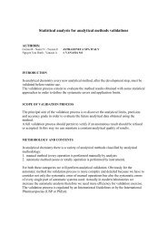
Figure 1 Two-period, two-treatment crossover
design
TYPICAL ANALYSIS
Data from a two-treatment, two-period crossover study are typically
analyzed using an analysis of variance (ANOVA) model with terms
for sequence, subject nested under sequence, treatment and
period. The carryover effect is, essentially, the sequence effect,
which is tested against the between subjects residual sum of
squares. Assuming the sequence effect (carryover) is not
significant, the basic ANOVA, with an equal numberof subjects (n)
in each sequence, takes the form shown in Table 1.
S
INTRODUCTION
Is it often the case that a pharmaceutical company will try to
develop a different formulation of a currently approved drug or
develop a different drug that is at least as effective as the standard
treatment, but is better in some facet, such as less side effects. In
such a case, the company is required to demonstrate that the two
treatments are bioequivalent ("same" rate and extentof absorption).
Typically, a two-period, two-treatment crossover study is conducted
for th is purpose.
Source of
variation
Sequence
Subject(sequence)
Treatment
Period
Error
Total
Degrees of
freedom (d.f.)
1
2(n·l)
1
2(n-l )
4n-1
STUDY DESIGN AND OBJECTIVES
In a two-period crossover design (Figure 1), subjects in one group
each receive a single dose of the standard treatment, while
subjects in another group receive the test treatment. After a
~washoue period, during which all traces of the drug are expected
to have disappeared from the body, each subject receives a dose
of the alternate formulation (period two). Thus, there would be,
say, n subjects in sequence group 1 who receive the standard
treatment in the first period and the test treatment in the second
period. In addition, there would be m (usually equal to n) subjects
in sequence group 2 who receive the test treatment first and then
the reference treatment. This design is appealing in that fewer
subjects are usually required than would be necessary for a
paraUel-groups design and each subject serves as hislher own
control.
The objective of the two-period crossover is usually the
determination of the equivalence of two treatments. Equivalence
here implies that the rate and extent of absorption of the two
treatments is essentially the Msame M • These absorption
characteristics are usually quantified in practice by means of area
under the blood level curve (AUG), peak drug concentration (Cmax)
Table 1 ANOVA for two-period, two-treatment
crossover design with n subjects per sequence
Some have given justification for automatically performing a
logarithmic (In) transformation on AUC and Gmax data before
performing the ANOVA. However, it is usually informative to
analyze the data both with and without transformation and examine
the residuals of each. One nice feature of In transforming is that
the confidence intervals constructed following the ANOVA will be
on ratios of means rather than differences, which fits into the
proportional form in which the FDA gives its rule for accepting
equivalence (±20%).
ASSESSMENT OF BIOEQUIVALENCE
Many methods for assessing bioequivalence have been proposed
over the years, some of which have been totally discarded and
others of which are still being studied and compared. Specifics of
the theory and methods used to test bioequivalence will not be
presented here. Anderson and Hauck (1983, 1984), Fluehler, etal
1423

(1981, 1983), locke (1984), Mandallaz and Mau (1981), Metzler
(1974, 1983, 1988, 1989), Rocke (1984, 1985), Rodda and Davis
(1980), Schuirmann (1987,1989), Selwyn and Hall (1984) and
Westlake (1972, 1976, 1981, 1988) are some of the available
references on the topic.
In some cases, the assessment of bioequivalence involves
estimating either the difference (test-standard) or ratio
(test/standard) of treatment means and forming a confidence
interval for the estimate. Equivalence is accepted if the confidence
interval is completely contained in some specified interval, (9 p 9:;J
In other cases, actual hypothesis tests are carried out and
bioequivalence is decided if the p-value of the null hypothesis is
less than some specified value, say 0.1. In still other cases, a
Bayesian posterior probability that the true value of the estimate
(difference or ratio) is contained in Some specified interval (8 1 ,9 2 )
is calculated, based on the sample values, and bioequivalence is
accepted if the posterior probability is greater than some level, say
0.95.
The current FDA recommended procedure is the two one-sided
testing approach which is operationally equivalent to construction
of a (1-2a.)100% confidence interval for the ratio of formulation
means. For non-transformed data, the confidence interval for the
ratio is commonly constructed by either dividing the endpoints of
the confidence interval for the difference in formulation means by
the reference sample mean (FDA method, see Report by the
Bioequivalence Task Force on recommendations from the
bioequivalence hearing conducted by the FDA, January 1988) or
by using Fieller's theorem. In addition, an exact method was
described by Locke (1984). If the data has undergone a
logarithmic transformation, a confidence interval for the ratio of test
to standard treatment can be easily calculated by exponentia~ng
the estimated difference and confidence interval endpOints.
SAS/AF SYSTEM
With the rather frequent occurrence of two-period crossover studies
for testing bioequivalence in our work environment, it was decided
to create an interactive, user-friendly SASJAF system to provide a
complete, start to finish analysis of such data; for use by
statisticians and non-statisticians alike. SAS/GRAPH@> and
SASISTAl" are utilized along with SAS/FSp·, SAS/AF and base
SA~ software. With this system in place, the time it takes to
analyze a set of data and provide a written report is greatly
reduced. Furthermore, overall conSistency in reports for different
data sets is attained.
The main menu of the SAS/AF system, displayed in Figure 2,
offers six choices. The SCl block fUnction was used to create this
selection screen.
I MAIN MENU I
IS~ps~_1
I D",ision
Aules I
I
Ulililies
I "" I I
Exil
I Data AnalysiS I
Place cursor on your selection and press the enter key.
Figure 2 Main menu of the SAS/AF Crossover Analysis
System
I
I
The system provides the capability to easily:
I s.np~wPM I
obtain sample size/power estimates for concluding
bioequivalence based on the (1-2a)100% confidence interval
approach (a~.05) (see Owen (1965) and Phillips (1990)J.
Estimates for both normal and log-normal data are available for
a variety of coefficients of variation and assumed underlying
differences in the treatment means, and two different
equivalence criteria. Estimates are contained in a SAS data set
and are obtained by subsetting the data set via where clauses.
The requested sample size or power estimate is displayed on
the screen.
'
I O~aAn~s I
analyze, plot, list, summarize, examine the need for
transformation, transform and reanalyze, test bioequivalence
and edit the data from a single dose, two-period, two-treatment
crossover study. The data from the study should be contained
in a SAS data set and should, at the least, contain variables for
subject. treatment, and some response to be analyzed.
I Decision Rules I
I Ulildjes
I
I
obtain a number of bioequivalence decision rules by inputting
only summary statistics from some previous analysis. Rules for
both non-transformed and In-transformed analyses are available
and results are presented in a tabular format.
I
edit/browse a SAS data set, assign a library reference, create
a SAS data set from an external file, and ediVbrowse the
names, formats, informats, and labels for the variables in a SAS
data set. This utility section allows users, unfamiliar with SAS,
to perform some basic, useful tasks.
H~p
I
obtain help on the system.
E~ ,
exit the system.
Full use of block style menus, push buttons, choice groups,
selection lists, and screen interaction capabilities is made
throughout the system. In addition, on-line help is available for all
screens and input fields. The help system was created as a
number of interconnecting CST entries to allow a user to
progressively advance through topics of interest.
Since the sample size/power and the data analysis sections are the
core of the system, they wilt be presented in more detail in the
remainder of the paper. No further information on the other
sections is provided.
Sample Size/Power
When the Samp Size/Pwr choice is selected from the main menu,
the input screen shown in Figure 3 displays. Each of the first three
lines contains a multi-station choice group, where .the user can
select one of the two choices offered. The cursor then
automatically advances to the fourth line, Percent difference in true
means, and the field is highlighted. Pressing on the
field displays a selection list of valid values from which the user
must make a selection.
1424

Depending on the specific selections made, other input lines
display, prompting the user for more information. For example, if
, and are
selected and a 5 percent difference in means is specified, the
screen would appear as shown in Figure 4.
With a coefficient of variation of 0.15 and a sample size of 20
selected, a power value of 0.91 is obtained and displayed on the
lower right hand side of the screen (Figure 5) when is
selected. Changes in the field values can be made and additional
estimates obtained. When the user is done, the section is ended
by pressing on at the bottom of the screen.
Control is returned to the main menu.
Data: cNormal· No Transformation:..
clog Transformed:.
Equivalence Criterion: c-+/·20%:0 c+l-25%:. (In data. ll=ln(.8))
Value Desired:

ANOVA model can be modified to delete non-significant terms if
desired. In addition to the usual analysis of variance output,
residual plots, PROC UNIVARIATE output on the residuals, and
Pitman-Morgan tests {see Morgan (1939) and Pitman (1939)] for
homogeneity of variance of treatments groups are also produced.
Data set: one.sample
Title Lines:
Data set: one.sample
Tille Une(s) for Listing:
Title Line(s) for Descriptive Statistics:
Select a transformation:
Reciprocal Inverse Square Root Naturallog Square Root Rank
Default model: trans(Y} '"' u + seq + period + trt + subject(seq) + error
Do you want to modify the model ('f or N) N
Place an X next to your selection(s):
_ include missing values in analysis
_ pool over treatments
_ pool over periods
Tab to desired statistics; press ENTER to selecttunseled:
MEAN N STD STDERR CV
VAR MAX MIN RANGE
Figure 8 Data listing and descriptive statistics
Select Option="".
Plot Menu
1 Plots of Parameters over Treatments
2 Plots of Parameters over Periods
Plots of Parameters over Treatments
and Periods
4 Plots of Test versus Reference
5 Return to Analysis Menu
Type your choice on the Select Option "'"''''> line and press ENTER.
Figure 9 Plot menu
PIal of L{A) VeI"SWI}.
hrultrr=CNU
-",-------------,
-u
-50 --- --~-~--------------- ---------
-1.5 -U -0.5 0.0 Q.5 1.0 1.5
L.d'.
-1--_____"-..... 1 .....-
Figure 10 Box-Cox plot with a 95% confidence interval
superimposed
Figure 11 Transformed analysis of variance
The Edit/Browse option in the analysis menu provides the
opportunity to analyze data with and without an outlying
observation, for example. Only the working data set is modified;
the original data set is left unchanged. This option takes
advantage of the call fsedit function in SCl.
Finally, once the data have been subjected to an ANOVA, either
non-transformed, transformed or both, summary tables and tables
of bioequivalence decision rules can be obtained. No input is
required for either of these functions, but a title line can be
provided if desired. Sample output tables are shown in Figures 12-
14.
CONCLUSION
The SAS/AF system presented here provides a means of
performing a rapid and accurate analysis of data from a twotreatment,
two-period crossover design. Sample size and power
estimates are available for a large variety of cases. Since the
determination of the equivalence of two treatments is usually the
main objective, the system provides easy access to several
decision rules, for both non-transformed and In-transformed data.
What rules are actually output depends on if an actual data set is
being analyzed or if only summary statistics from some previous
analysis are available. The treatment ratio estimates are output,
along with confidence intervals or probability values, in a ready to
use table. ANOVA output (original andlor transformed), a variety
of plots of the data, Box-Cox plots, tables of summary statistics and
tables summarizing the analyses performed can also be created
and output to files for further use in reports. In addition, the system
can perform a number of basic utility functions that allow the user
to execute certain tasks without leaving the system.
The separate components of the SAS system that are used in this
system, such as SAS/STAT, SAS/GRAPH, and base SASsoftware,
provide all the functions needed to analyze and plot the type of
data presented here. However, by using SAS/AF and sel to
create a user-friendly front end and to make the system completely
interactive, it was possible to develop a very powerful, concise
system specific enough for the study type of interest, but general
enough to allow for differences in data sets, variables, and analysis
choices. Furthermore, the system can easily be run by persons
having no actual SAS programming skills and little statistical
background.
SAS, SAS/AF, SAS/FSP, SAS/GRAPH and SAS/STAT are
registered trademarks of SAS Institute Inc. in the USA and other
countries. ® indicates USA registration.
1426

Figure 12 Summary table for non-transformed parameters
DECISION RULES FOR BIOEQUIVALENCE - UNTRANSFORMED
POINT (TIA) LOWER UPPER
PARAMETER !!!:&£ ESTIMATE
!!!::1!I 1!.M!!
PROB DECISION
AUC
CMAX
90% CONFIDENCE INTERVAL
Approx. FDA 1.027 0.871 1.183 B
Fixed Fleller 1.027 0.880 1.199 B
Exact Locke 1.027 0.877 1.194 B
BAYESIAN POSTERIOR PROB.
MandaUaz 8: Mau 1.027 0.941
90% CONFIDENCE INTERVAL
Approx. FDA 1.087 0.904 1.270
Fixed Fieller 1.087 0.912 1.299
Exact Locke 1.087 0.919 1.346
BAYESIAN POSTERIOR PROS.
Mandallaz 8: Mau 1.087 0.834
B = Bioequivalence
I = Bio-Inequivalence
Figure 13 Table of Bioequivalence Decision Rules for non-transformed parameters
DECISION RULES FOR BIOEQUIVAlENCE - LN TRANSFORMED
POINT (TiA) LOWER UPPER
PARAMETER RULE ESTIMATE
1!M!.!. LIMIT ~ DECISION
TAUC
TCMAX
90% CONADENCE INTERVAL
FDA 1.032 0.873 1.220
BAYESIAN POSTERIOR PROS.
Mandallaz 8: Mau 1.032 0.922
90% CONFIDENCE INTERVAL
FDA 1.144 0.957 1.367
BAYESIAN POSTERIOR PROB.
Mandallaz 8: Mau 1.144 0.686
B = Bioequivalence
I = Bio-Inequivalence
Figure 14 Table of Bioequivalence Decision Rules for In-transformed parameters
1427

ACKNOWLEDGEMENTS
Thanks go to Rita Kristy, Sharon Trevoy, Fred Snikeris and Gary
Stevens, members of the Preclinical and Scientific Statistics
Department at Sterling Winthrop Inc., for their contributions to the
development of the methodology and to the design of the SAS/AF
system.
REFERENCES
Anderson, S. and W.W. Hauck (1983). A new procedure for testing
equivalence in comparative bioavailabili~ and other clinical trials.
Communications in Statistics - TheoretJcaJ Methods 12, 2663-
2692.
Anderson, S. and W.W. Hauck (1984). A new statistical procedure
for testing equivalence in two-group comparative bioavailability
trials. Journal of Pharmacokinetics and Biopharmaceutics 12, 83-
90.
Box, G.E.P., and D.R. Cox (1964). An analysis of transfonnations.
J. Royal Stat. Soc. B26, 211-252.
Fluehler, H., J. Hirtz, and H.A. Moser (1981). An aid to decision
making in bioequivalence assessment. Journal of
Pharmacokinetics and Biopharmaceutics 9, 235-243.
Fluehler, H., A.P. Grieve, D. Mandallaz, J. Mau, and H.A. Moser
(1983). Bayesian approach to bioequivalence assessment: An
e-xample. Journal of Pharmaceutical Sciences 72, 1178-1181.
Haaland, P.O. (1989). Experimental Design in Biotechnology. New
York: Marcel Dekker, Inc.
Locke, C.S. (1984). An exact confidence interval from
untransformed data for the ratio of two formulation means.
Journal of Pharmacokinetics and Biopharmaceutics 12, 649-655.
Mandallaz, D. and J. Mau (1981). Comparison of different methods
for decision-making in bioequivalence assessment. Biometrics
37, 213-222.
Metzler, C.M. (1974). Bioavailability - a problem in equivalence.
Biometrics 30,309-317.
Metzler, C.M. and D.C. Huang (1983). Statistical methods for
bioavailability and bioequivalence. Clinical Research Practices
& Drug Regulatory Affairs 1, 109-132.
Metzler, C.M. (1988). Statistical methods for deciding
bioequivalence of formulations. In Oral Sustained Release
Formulations: Design and Evaluation.
Pitman, E.J.G. (1939). A note on normal correlation. Biometrika
31,9-12.
Rocke, D.M. (1984). On testing for bioequivalence. Biometrics 40,
225-230.
Rocke, D.M. (1985). On testing for bioequivalence: Letter to the
Editor. Biometrics 41, 561-563.
Rodda, B.E. and R.l. Davis (1980). Determining the probability of
an important difference in bioavaHability. Clinical Pharmacology
Ther. 28, 247-252.
Schuirmann, D.J. (1987). A comparison of the two one-sided tests
procedure and the power approach for assessing the
equivalence of average bioavailability. Journal of
Pharmacokinetics and Biopharmaceutics15, 657-680.
Schuirmann, D.J. (1989). Confidence intervals for the ratio of two
means from a crossover study. Paper presented at the
American Statistical Association Annual Meeting, August, 1989,
Anaheim, CA.
Selwyn, M.R. and N.R. Hall (1984). On Bayesian methods for
bioequivalence. Biometrics 40, 1103-1108.
Weisberg, S. (1985). Applied Unear Regression, second edition.
New York:. John Wiley & Sons, Inc.
Westlake, W.J. (1972). Use of confidence intervals in analysis of
comparative bioavailability trials. Journal of Pharmaceutical
Sciences 61,1340-1341.
Westlake, W.J. (1976). Symmetrical confidence intervals for
bioequivalence trials. Biometrics 32, 741-744.
Westlake, W.J. (1981). Bioequivalence testing - a need to rethink.
Biometrics 37, 589-594.
Westlake, W.J. (1988). Bioavailability and bioequivalence of
pharmaceutical formulations. In Biopharmaceutical Statistics for
Drug Development. K. Peace (ed.), New York: Marcel Dekker.
Author:
Deborah Dukovic, Statistician
Sterling Winthrop, Inc.
9 Great Valley Parkway
Malvern, PA 19355
(215) 889-8665
Metzler, C.M. (1989). Bioavailabilitylbioequivalence: study design
and statistical issues. Journal of Clinical Pharmacology 29, 289-
292.
Morgan, W.A. (1939). A test for the significance of the difference
between the two variances in a sample from a normal bivariate
population. Biometrika 31, 13-19.
Owen, 0.8. (1965). A special case of a bivariate non-central t­
distribution. Biometrika 52,437-446.
Phillips, K.F. (1990). Power of the two one-sided lests procedure
in bioequivalence. Journal of Pharmacokinetics and
Biopharmaceutics 18, 137-144.
1428