Determination of partial factors for vertically loaded piles for a ...
Determination of partial factors for vertically loaded piles for a ...
Determination of partial factors for vertically loaded piles for a ...

Create successful ePaper yourself
Turn your PDF publications into a flip-book with our unique Google optimized e-Paper software.
JCSS<br />
Workshop on Reliability Based Code Calibration<br />
<strong>Determination</strong> <strong>of</strong> <strong>partial</strong> <strong>factors</strong> <strong>for</strong> <strong>vertically</strong> <strong>loaded</strong> <strong>piles</strong><br />
<strong>for</strong> a seismic loading condition based on reliability theory<br />
Yusuke Honjo Shailendra Amatya Makoto Suzuki Masahiro Shirato<br />
Gifu University,<br />
Gifu, Japan<br />
Gifu University,<br />
Gifu, Japan<br />
Shimizu Corporation,<br />
Tokyo, Japan<br />
1<br />
Public Works<br />
Research Institute,<br />
Tsukuba, Japan<br />
Abstract<br />
The aim <strong>of</strong> this study is to establish a procedure in the limit state design <strong>for</strong>mat to<br />
rationally determine the <strong>partial</strong> <strong>factors</strong> <strong>for</strong> a <strong>vertically</strong> <strong>loaded</strong> pile based on a sound<br />
reliability theory. The frequency <strong>of</strong> the usage <strong>of</strong> pile types and dimensions are<br />
investigated first. Several design examples are selected, and load ranges and<br />
combinations on typical <strong>piles</strong> are studied. Based on these results, typical load<br />
intensities, load combinations and soil pr<strong>of</strong>iles are set <strong>for</strong> the code calibration. Also<br />
uncertainties involved in seismic loading are investigated based on the historical<br />
seismic data using an extreme statistical analysis, so called POT (peaks over<br />
threshold) analysis. Uncertainties concerning resistances <strong>of</strong> <strong>piles</strong> are taken from a<br />
well-known study by Okahara et al (1991). FORM (first order reliability method)<br />
analysis is carried out to find out the current level <strong>of</strong> reliability index. Finally, the<br />
design value method is employed to determine the <strong>partial</strong> <strong>factors</strong>.<br />
Keywords: pile design, vertical bearing capacity, <strong>partial</strong> <strong>factors</strong>, safety factor,<br />
reliability analysis, FORM, extreme statistics, POT analysis, code calibration<br />
1 Introduction<br />
1.1 Background<br />
It is recognized widely that one <strong>of</strong> the origins <strong>of</strong> the introduction <strong>of</strong> the limit design<br />
concept started in Denmark in 1960s by the ef<strong>for</strong>t <strong>of</strong> Brinch-Hansen (1967). By<br />
1970s, Danish geotechnical design code has been based on the limit state design<br />
concept and <strong>partial</strong> <strong>factors</strong> were introduced. It is considered that Eurocode 7 (CEN,<br />
1994) was much influenced by this code (Meyerh<strong>of</strong> 1993; Ovesen, 1993).<br />
The introduction <strong>of</strong> the limit state design concept, which is sometimes called Load<br />
and Resistance Factors Design (LRFD), is also coming to be popular in North<br />
America. Such works includes Barker et al (1991), AASHTO (1994), Becker (1996)<br />
and Phoon, Kulhawy and Grigoriu (1995 and 2000).<br />
Gobel (1999) has summarized the works done in this area, especially in North<br />
America, and concluded that most <strong>of</strong> the works done in 1990s still contain some<br />
degree <strong>of</strong> vagueness in the determination <strong>of</strong> resistance <strong>factors</strong>. He further<br />
emphasizes the use <strong>of</strong> available databases and rational probabilistic analysis to<br />
determine the <strong>partial</strong> <strong>factors</strong>.
JCSS<br />
Workshop on Reliability Based Code Calibration<br />
Paikowsky and Stenersen (2000) who are working <strong>of</strong> revision <strong>of</strong> the AASHTO driven<br />
pile design procedure are proposing a method to design <strong>piles</strong> based on<br />
measurements during pile driving. They have carried out extensive statistical<br />
analysis on a large database, and <strong>partial</strong> <strong>factors</strong> are proposed based on this result.<br />
In Japan, conversions <strong>of</strong> the current design codes to ones based on the limit state<br />
design concept are very much activated (see Honjo et al, 2000). All the major<br />
foundation design codes seem to be aiming at the limit state design code and<br />
per<strong>for</strong>mance based design concepts.<br />
1.2 Objectives <strong>of</strong> this study<br />
The objective <strong>of</strong> this study is to establish a procedure to rationally determine the<br />
<strong>partial</strong> <strong>factors</strong> <strong>for</strong> a <strong>vertically</strong> <strong>loaded</strong> pile in the limit state design <strong>for</strong>mat based on a<br />
sound reliability theory. We would employ pile design method specified in<br />
“Specifications <strong>for</strong> Highway Bridges IV: Substructures” (JRA, 1996), denoted as SHB<br />
(1996) hereafter.<br />
This conventional design method can be rewritten in a simplified <strong>for</strong>m as follows:<br />
1<br />
( Rt<br />
+ Rs<br />
) ≥ Sd<br />
+ Se<br />
(1)<br />
Fs<br />
where Rt and Rs are pile tip and pile side resistances, Rs being considered <strong>for</strong> two<br />
cases: in sand and in cohesive soil, whereas, Sd and Se are vertical pile top <strong>for</strong>ces<br />
induced by dead load and seismic <strong>for</strong>ce.<br />
In the <strong>partial</strong> factor <strong>for</strong>mat <strong>for</strong> which we are going to carry out calibration, the <strong>partial</strong><br />
<strong>factors</strong> are applied to dead and seismic loads as well as pile tip and side resistances<br />
which can be <strong>for</strong>mulated as the follows:<br />
γ R + γ R ≥ γ S + γ S<br />
(2)<br />
Rt<br />
t<br />
Rs<br />
s<br />
Sd<br />
d<br />
Se<br />
e<br />
where γRt, γRs, γSd and γSe are <strong>partial</strong> <strong>factors</strong> <strong>for</strong> the resistances and the <strong>for</strong>ces<br />
respectively.<br />
2 Frequent load ranges, combinations and soil pr<strong>of</strong>iles<br />
2.1 Type and size <strong>of</strong> <strong>piles</strong> used in highway bridge foundations in<br />
Japan<br />
Fukui et al (1996) has carried out an investigation based on a questionnaire to study<br />
the details <strong>of</strong> highway bridge foundations in Japan. The investigation period was<br />
from November 1995 to January 1996. 4,995 bridge foundations were investigated<br />
<strong>of</strong> which 2,441 were ordinary pile foundations.<br />
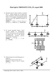
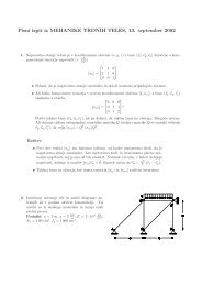
Presented in Fig. 1(a) is distribution <strong>of</strong> pile types among these 2,441 cases where<br />
about 70% consists <strong>of</strong> cast-in place <strong>piles</strong>, 24% steel <strong>piles</strong> and 5% PHC (pre-stressed<br />
high strength concrete) <strong>piles</strong>. The frequency <strong>of</strong> the cast-in place pile is considerably<br />
high due to the environmental restrictions during construction, such as noise and<br />
vibration. Due to the extraordinary high usage frequency <strong>of</strong> cast in-situ pile, only<br />
these types <strong>of</strong> <strong>piles</strong> are considered in this study.<br />
2
JCSS<br />
The distribution <strong>of</strong> pile diameters <strong>of</strong> the<br />
1,734 cast in-situ <strong>piles</strong> is shown in<br />
Fig. 1(b). Although some <strong>piles</strong> have<br />
diameter <strong>of</strong> 200 cm, more than 95% <strong>of</strong><br />
them have diameter between 100 to 150<br />
cm. Concerning the length <strong>of</strong> the cast-in<br />
place <strong>piles</strong>, about 85% <strong>of</strong> them distribute<br />
between 6 to 30 m as presented in<br />
Fig. 1(c).<br />
2.2 Characteristics <strong>of</strong> the load<br />
ranges and combinations<br />
and the chosen cases<br />
Based on the investigation on usage frequency<br />
<strong>of</strong> the <strong>piles</strong> <strong>for</strong> highway bridge<br />
foundations, 8 pile foundation design<br />
examples <strong>of</strong> cast-in place <strong>piles</strong> are selected<br />
<strong>for</strong> more detailed study on load<br />
ranges and combinations. The pile<br />
diameter ranges between 100 to 150 cm<br />
and the length 9.5 to 35.5 m. The<br />
ranges conveniently cover the most<br />
frequent dimensions <strong>of</strong> the commonly<br />
used cast in-situ <strong>piles</strong>.<br />
In 7 among the 8 examples chosen, the<br />
critical loading condition is seismic loading<br />
in L1 (Level 1) seismic situation 1 . In<br />
only one case, the pile diameter is determined<br />
by the L2 seismic <strong>for</strong>ce. Mainly<br />
<strong>for</strong> this reason, the <strong>partial</strong> <strong>factors</strong> are<br />
only calibrated <strong>for</strong> L1 case in this study.<br />
Since L1 seismic loading situation is the<br />
most critical <strong>for</strong> vertical loading <strong>of</strong> the<br />
most <strong>of</strong> pile foundations, the vertical load<br />
intensity and load combinations <strong>of</strong> this<br />
situation <strong>for</strong> the most critical <strong>piles</strong> in<br />
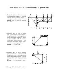
each foundation example are plotted in<br />
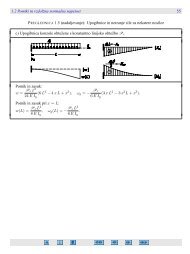
Fig. 2 2 .<br />
Workshop on Reliability Based Code Calibration<br />
1 In SHB(1996), two seismic situations are considered: L1 (Level 1)earthquakes whose occurrences<br />
are expected to be several times during the service life <strong>of</strong> a structure. L2 (Level 2) earthquakes are<br />
much larger earthquakes whose occurrences are not certain during the service life. SHB specifies that<br />
seismic coefficient method be used <strong>for</strong> L1 earthquakes, whereas the ductility design method be<br />
employed <strong>for</strong> L2 (JSCE, 2000).<br />
2 The vertical dead and seismic loads <strong>for</strong> the most critical <strong>piles</strong> in chosen pile foundations are<br />
calculated based on SHB specified calculation model. The model is basically rigid frame supported by<br />
vertical and horizontal subgrade reaction springs, and the loads, namely vertical, horizontal and<br />
moment, are applied at the center <strong>of</strong> footing as concentrated loads. In this calculation, the most<br />
critical <strong>piles</strong> are ones in the front row <strong>of</strong> the pile foundation.<br />
3<br />
Ratio (%)<br />
Frequency<br />
Frequency<br />
100<br />
80<br />
60<br />
40<br />
20<br />
1000<br />
800<br />
600<br />
400<br />
200<br />
500<br />
400<br />
300<br />
200<br />
100<br />
0<br />
0<br />
0<br />
69.2<br />
630<br />
1<br />
23.5<br />
773<br />
(b) Pile diameter (cast in-situ pile)<br />
3<br />
4.7 2.6<br />
Cast in- Steel <strong>piles</strong> PHC <strong>piles</strong> Other<br />
situ <strong>piles</strong><br />
Pile types<br />
(a) Pile types<br />
types<br />
266<br />
1<br />
58<br />
100 110 120 124 150 180 200<br />
Diameter (cm)<br />
33<br />
5 or less<br />
416 387<br />
6 to 10<br />
11 to 15<br />
317 364<br />
16 to 20<br />
21 to 30<br />
144<br />
31 to 40<br />
Pile length (m)<br />
(c) Pile length (Cast-in situ pile)<br />
61<br />
41 to 50<br />
9<br />
51 to 60<br />
Fig. 1. Piles used in Japanese highway<br />
bridge foundations (after Fukui et al, 1996)
JCSS<br />
It is a common practice to check the pile<br />
dimensions <strong>for</strong> two cases, namely the<br />
case when buoyancy is considered<br />
(assuming ground water level coincide<br />
with the ground surface) and the case<br />
when buoyancy is ignored. The load<br />
ranges and load combinations <strong>for</strong> the<br />
first case is shown in Fig. 2. It is observed<br />
in the figure that the range <strong>of</strong> the<br />
dead load lies from 500 to 2500 kN, so<br />
that the seismic vertical load ranges<br />
from 500 to 3,500 kN. The regression<br />
line <strong>for</strong> the mean <strong>of</strong> the dead load vs. the<br />
seismic load is Se = 1.2 Sd as indicated<br />
in the figure with the one standard<br />
deviation <strong>of</strong> Se = (1.2 ± 0.3) Sd.<br />
Essentially the same results are<br />
Workshop on Reliability Based Code Calibration<br />
obtained <strong>for</strong> the case where buoyancy is ignored: in this case, the regression line is<br />
given as Se = (1.4±0.4) Sd.<br />
Based on the results <strong>of</strong> the load range and the combinations found in Fig. 2, 21<br />
loading cases are set in the following way:<br />
1. The basic vertical loads are chosen. In regard to the load intensity range<br />
observed in Fig. 2, vertical loads <strong>of</strong> 500, 1000, 1500, 2000 and 2500 kN are<br />
chosen.<br />
2. For each vertical load, seismic loads are determined based on the regression<br />
lines presented in Fig. 2: 3 different kinds <strong>of</strong> seismic induced vertical <strong>for</strong>ces are<br />
set which are denoted by u, a and l (upper, average and lower). Thus, the cases<br />
are denoted as, <strong>for</strong> example, 500.u, 2000.a etc.<br />
3. For each case, a pile has to be designed <strong>for</strong> dead load and seismic induced<br />
vertical load under conditions considering and ignoring the buoyancy: they are<br />
indicated, <strong>for</strong> example, 500.u-bc (buoyancy considered), 2000.a-bn (buoyancy<br />
neglected).<br />
4. Two cases are set <strong>for</strong> 1500 and 2000 considering the higher frequency <strong>of</strong> the<br />
usage <strong>of</strong> the <strong>piles</strong> in these, whereas only one case is set <strong>for</strong> the others, i.e. 500,<br />
1000 and 2500.<br />
5. The soil pr<strong>of</strong>iles are set <strong>for</strong> the loading cases based on the selected pile<br />
foundation design examples described previously. They are believed to<br />
represent the variety <strong>of</strong> pr<strong>of</strong>iles encountered in pile foundation design in Japan.<br />
2.3 Designed pile lengths and diameters by the conventional<br />
method<br />
Piles are designed <strong>for</strong> each case set in the previous section based on the design<br />
method specified in SHB (1996). The designed diameters <strong>of</strong> <strong>piles</strong> are not rounded<br />
<strong>of</strong>f as are commonly done in practice, but left in the order <strong>of</strong> centimetres (cm). In the<br />
all cases, the diameters are determined <strong>for</strong> the cases pile buoyancy being neglected.<br />
In other words, L2 seismic situations are not critical in determining the dimensions <strong>of</strong><br />
<strong>piles</strong>.<br />
4<br />
Se (kN)<br />
5000<br />
4000<br />
3000<br />
2000<br />
1000<br />
0<br />
0 500 1000 1500 2000 2500 3000<br />
Sd (kN)<br />
Fig. 2. Dead loads vs. seismic loads
JCSS<br />
Workshop on Reliability Based Code Calibration<br />
3 Uncertainties in basic variables<br />
3.1 Uncertainties in the loads<br />
3.1.1 Dead load<br />
An investigation was carried out by Japan Road Association on uncertainty involved<br />
in the unit weight <strong>of</strong> rein<strong>for</strong>ced concrete. It was concluded that the error in the unit<br />
weight follows a normal distribution with mean 1.0 and s.d. 0.015 (JRA, 1989). In this<br />
study, a normal distribution with mean 1.0 and s.d. 0.1 is assumed <strong>for</strong> the uncertainty<br />
<strong>of</strong> dead load. It will be seen later that with this magnitude <strong>of</strong> uncertainty, the dead<br />
load has very little influence on the results <strong>of</strong> the reliability analysis.<br />
3.1.2 Seismic load<br />
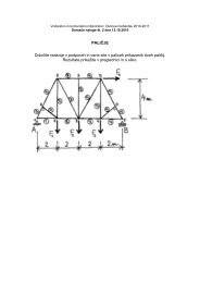
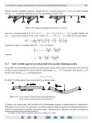
To estimate the uncertainties in the seismic load, based on Usami catalogue (Usami,<br />
1997), the seismic data <strong>for</strong> the years 1600 to 1995 have been taken. Distances from<br />
the location <strong>of</strong> Tokyo Metropolis Hall to the epicentres are calculated. The<br />
accelerations <strong>for</strong> all the earthquakes from the data at distances deduced above are<br />
then calculated using Fukushima-Tanaka (1991) attenuation model, and yearly<br />
maximum accelerations extracted. Fig. 3 shows the yearly maximum acceleration<br />
obtained <strong>for</strong> Tokyo.<br />
The peaks over threshold (POT) analysis is employed in this study. In the POT<br />
analysis, the data over a relatively high threshold value, say u, are fitted to an<br />
exceedance distribution <strong>of</strong> u, F [u] (x). According to the theory by Balkema and de<br />
Hann (1974) and Pickands (1975), this can be well approximated by a General<br />
Pareto distribution, W(⋅), provided the threshold tends to the right endpoint <strong>of</strong> the<br />
distribution <strong>of</strong> data (Reiss & Thomas, 1997).<br />
F u [ ]<br />
F1(<br />
x)<br />
− F(<br />
u)<br />
( x)<br />
= P(<br />
X ≤ x | X > u)<br />
=<br />
, x ≥ u<br />
1−<br />
F(<br />
u)<br />
−1<br />
γ<br />
[ ] ⎛ x − u ⎞ ⎛ x − u ⎞<br />
F ( x)<br />
= W ⎜ ⎟ = 1−<br />
⎜1+<br />
γ ⎟<br />
⎝ σ ⎠ ⎝ σ ⎠<br />
u<br />
(3b)<br />
From these, using Hazen plot identity, we can then derive the following equation as<br />
the distribution function <strong>of</strong> the annual maximum:<br />
5<br />
(3a)<br />
n k k ⎡<br />
− 1<br />
γ<br />
+ 1−<br />
⎛ x − u ⎞<br />
⎤<br />
F x<br />
⎢<br />
⎟ ⎥<br />
1(<br />
) = + 1−<br />
⎜1+<br />
γ ⋅<br />
valid <strong>for</strong> x ≥ u<br />
(4)<br />
n + 1 n + 1⎢<br />
⎣<br />
⎝ σ ⎠ ⎥<br />
⎦<br />
where n = total number <strong>of</strong> observations, k = number <strong>of</strong> exceedances (or the number<br />
<strong>of</strong> data with x ≥ u), γ = shape parameter and σ = scale parameter <strong>of</strong> General Pareto<br />
distribution, u is the location parameter.<br />
The threshold values, u, are decided using exploratory data analysis tools as mean<br />
excess function (MEF) plot, γ-estimate plot and qq-plot.<br />
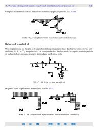
Sample MEF plot, Fig. 4(b), is a precursor <strong>of</strong> the heavy-tailed distribution which<br />
could be best fit to the data; the MEF <strong>of</strong> a Pareto distribution is a straight line with an<br />
increasing trend. Hence, the threshold value in our case shall be decided from the
JCSS<br />
Workshop on Reliability Based Code Calibration<br />
portion <strong>of</strong> the plot within which the sample MEF “looks linear”, and leave out the<br />
heavier-tailed portion deviating from it (Bassi, 1998).<br />
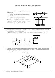
The γ-estimate plots obtained <strong>for</strong> different estimates <strong>of</strong> General Pareto distribution as<br />
maximum likelihood estimate (MLE), moment estimate (Moment) and Drees-<br />
Pickands estimate (D-P) are actually used to choose the thresholds. As can be seen<br />
in Fig. 4(a), these plots have “plateaus” or “peaks”. The regions <strong>of</strong> stable parameter<br />
estimates are one <strong>of</strong> these (Reiss, 1997). XTREMES s<strong>of</strong>tware (Reiss & Thomas,<br />
1997) was used to estimate the distribution parameters.<br />
The estimated parameters finally introduced in this study are as follows: n = 396, k =<br />
99, γ = 0.070, u = 26.66 and σ = 80.45. Fig. 4(c) shows the cumulative distribution<br />
functions <strong>of</strong> this estimated distribution and the sample data. The resulting 50, 100<br />
and 500-year expected values are 320, 490 and 570 gals respectively (Honjo &<br />
Amatya, 2001).<br />
seismic acceleration, x (gals)<br />
Fig. 3. Yearly maximum acceleration <strong>for</strong> Tokyo by Fukushima-Tanaka attenuation<br />
model (1991) based on Usami catalogue.<br />
-estimates<br />
350<br />
300<br />
250<br />
200<br />
150<br />
100<br />
50<br />
0<br />
1<br />
0.8<br />
0.6<br />
0.4<br />
0.2<br />
0<br />
-0.2<br />
-0.4<br />
-0.6<br />
-0.8<br />
1600<br />
1620<br />
1640<br />
1660<br />
1680<br />
1700<br />
Drees-Pickands estimates<br />
Moment estimates<br />
0 20 40 60 80 100 120 140 160 180 200<br />
Number <strong>of</strong> exceedances, k<br />
Fig. 4(a). γ-plots <strong>for</strong> yearly maximum acceleration <strong>for</strong> Tokyo<br />
1720<br />
1740<br />
1760<br />
1780<br />
6<br />
1800<br />
1820<br />
1840<br />
1860<br />
1880<br />
1900<br />
1920<br />
MLE estimates<br />
1940<br />
1960<br />
1980
Mean excess function, e (u )<br />
100<br />
80<br />
60<br />
40<br />
20<br />
JCSS<br />
Workshop on Reliability Based Code Calibration<br />
0 50 100 150 200<br />
Excess acceleration, u (gals)<br />
The obtained 100-year expected maximum acceleration is assumed to induce the<br />
seismic <strong>for</strong>ce that is employed in SHB (1996) L1 situation. In the reliability analysis,<br />
the reference period <strong>of</strong> a structure is assumed to be 100 years. Thus, the 100-year<br />
maximum seismic <strong>for</strong>ce distribution is obtained from Eq.(4) as follows:<br />
100<br />
⎛ x ⎞ ⎛ S ⎡<br />
⎤<br />
e ⎞ ⎛ Se<br />
⎞<br />
100 ( S ) 100 ⎜<br />
. 1 ⎟ = 100 ⎜ ⋅ 100 ⎟ = ⎢ 1 ⎜ ⋅ 100 ⎟<br />
e = G ⋅S<br />
e L F x F x ⎥ (5)<br />
⎝ x100<br />
⎠ ⎝ Se.<br />
L1<br />
⎠ ⎝ Se.<br />
L1<br />
⎠⎦<br />
G<br />
⎣<br />
where G100(Se) is the 100-year maximum seismic <strong>for</strong>ce distribution, Se is the seismic<br />
<strong>for</strong>ce, x is the maximum ground surface acceleration, x100 is the 100-year expected<br />
maximum ground surface acceleration, Se.L1 is the seismic <strong>for</strong>ce used in SHB (1996)<br />
<strong>for</strong> L1 seismic situation, F100 is the distribution function <strong>of</strong> 100-year maximum ground<br />
surface acceleration, and F1 is the distribution function <strong>of</strong> the annual maximum<br />
ground surface acceleration.<br />
3.2 Uncertainties in resistances<br />
Okahara et al (1991) tried to separately evaluate uncertainties in the SHB vertical pile<br />
bearing capacity calculation <strong>for</strong>mula on unit pile tip resistance, qd, and unit side<br />
resistance, f, based on the available pile loading tests data with respect to SPT<br />
N-values.<br />
First they defined the failure load <strong>of</strong> a pile as the load when vertical displacement <strong>of</strong><br />
the governments and the public authorities. Due to the fact that not all the cases<br />
provided all the necessary in<strong>for</strong>mation, only 32 cases could be put into analysis to<br />
evaluate the uncertainties <strong>for</strong> pile tip and side resistances <strong>for</strong> cast-in place pile.<br />
Shown in Table 1 are the results <strong>for</strong> cast in-situ <strong>piles</strong>. It is one <strong>of</strong> the distinguished<br />
features <strong>of</strong> their results that the biases <strong>of</strong> the calculated bearing capacity is small, i.e.<br />
1.07 and 1.12 <strong>for</strong> pile tip and side resistances. The c.o.v.'s are very high: 0.46 and<br />
0.63 respectively. They have carried out χ 2 fitness tests to the obtained distributions,<br />
and found they can be approximated either by normal distribution or lognormal<br />
distribution with the significance level <strong>of</strong> 5%.<br />
7<br />
F (x)<br />
1.00<br />
0.95<br />
0.90<br />
0.85<br />
0.80<br />
0.75<br />
0.70<br />
k = 99<br />
data<br />
MLE est.<br />
0 100 200 300<br />
x (gals)<br />
400 500 600<br />
Fig. 4(b). Sample MEF plot and Fig. 4(c). CDFs <strong>of</strong> estimated distribution and sample data
JCSS<br />
Workshop on Reliability Based Code Calibration<br />
Table 1. Uncertainties in the basic variables by Okahara et al (1991).<br />
Notation Definition <strong>of</strong> variables<br />
δf<br />
δqd<br />
δN<br />
Side resistance estimated based on the<br />
following <strong>for</strong>mula:<br />
f = 4 N (
JCSS<br />
Workshop on Reliability Based Code Calibration<br />
Table 2. Calculated <strong>partial</strong> <strong>factors</strong> by the design value method and the direct method<br />
Case<br />
Vertical<br />
dead<br />
load<br />
Vertical<br />
Diameter Length<br />
seismic<br />
<strong>of</strong> pile <strong>of</strong> pile<br />
load<br />
Sd (kN) Se (kN) D (m)<br />
L(m<br />
)<br />
Reliability<br />
Index<br />
Partial <strong>factors</strong> by the design<br />
value method<br />
9<br />
Partial <strong>factors</strong> directly<br />
calculated from the design<br />
values<br />
β γSd γSe γRt γRs γ * Sd γ * Se γ * Rt γ * Rs<br />
500.u 900 0.85 8.0 1.66 1.00 1.13 0.62 0.79 1.01 2.24 0.83 0.92<br />
500.a 500 700 0.77 8.0 1.77 1.01 1.13 0.62 0.78 1.01 2.33 0.82 0.91<br />
500.l<br />
500 0.68 8.0 1.91 1.01 1.12 0.63 0.76 1.02 2.45 0.81 0.88<br />
1000.u.1 1800 0.97 14.0 1.73 1.00 1.14 0.71 0.73 1.01 2.36 0.90 0.87<br />
1000.a.1 1000 1400 0.86 14.0 1.81 1.01 1.13 0.72 0.71 1.02 2.43 0.90 0.85<br />
1000.l.1<br />
1000 0.75 14.0 1.92 1.01 1.12 0.73 0.70 1.02 2.57 0.89 0.82<br />
1500.u.1 2700 0.91 27.5 1.64 1.00 1.13 0.79 0.69 1.01 2.22 0.96 0.85<br />
1500.a.1 1500 2100 0.8 27.5 1.74 1.01 1.12 0.79 0.67 1.01 2.29 0.96 0.83<br />
1500.l.1<br />
1500 0.68 27.5 1.88 1.01 1.11 0.80 0.65 1.02 2.36 0.96 0.80<br />
1500.u.2 2700 1.05 27.0 1.68 1.00 1.13 0.75 0.70 1.01 2.27 0.93 0.86<br />
1500.a.2 1500 2100 0.92 27.0 1.76 1.01 1.13 0.76 0.69 1.01 2.32 0.93 0.84<br />
1500.l.2<br />
1500 0.79 27.0 1.90 1.01 1.12 0.76 0.67 1.02 2.42 0.93 0.81<br />
2000.u.1 3600 1.45 22.5 1.70 1.00 1.13 0.69 0.73 1.01 2.29 0.88 0.88<br />
2000.a.1 2000 2800 1.29 22.5 1.79 1.01 1.13 0.70 0.72 1.02 2.36 0.88 0.86<br />
2000.l.1<br />
2000 1.12 22.5 1.93 1.01 1.12 0.70 0.70 1.02 2.48 0.87 0.83<br />
2000.u.2 3600 1.41 14.0 1.33 1.01 1.13 0.65 0.74 1.01 1.91 0.90 0.92<br />
2000.a.2 2000 2800 1.26 14.0 1.41 1.01 1.12 0.66 0.73 1.01 1.96 0.89 0.90<br />
2000.l.2<br />
2000 1.09 14.0 1.50 1.01 1.10 0.66 0.70 1.02 1.99 0.88 0.88<br />
2500.u 4500 1.41 23.5 1.67 1.00 1.13 0.73 0.71 1.01 2.27 0.92 0.86<br />
2500.a 2500 3500 1.24 23.5 1.75 1.01 1.13 0.74 0.69 1.01 2.32 0.92 0.84<br />
2500.l<br />
2500 1.07 23.5 1.90 1.01 1.12 0.75 0.67 1.02 2.43 0.92 0.81<br />
mean 1.73 1.01 1.13 0.71 0.71 1.02 2.30 0.90 0.86<br />
s.d. 0.16 0.00 0.01 0.06 0.03 0.00 0.17 0.04 0.04<br />
The sensitivity <strong>factors</strong>, α's, <strong>for</strong> the dead load, Sd, lies between -0.05 to -0.10, which<br />
essentially can be considered insensitive in the current reliability analysis. In<br />
contrast, those <strong>for</strong> the seismic load exhibit values between -0.82 to -0.87, which are<br />
significant and fall in relatively narrow range. On the other hand, those <strong>of</strong> the pile tip<br />
and side resistance, Rt and Rs, lie between 0.17 to 0.42 and 0.27 to 0.52 respectively.<br />
In the present study, it is intended that the newly developed design <strong>for</strong>mula should<br />
have equivalent safety margin compared to the conventional design <strong>for</strong>mula. For this<br />
reason, the target reliability index, βT, is set to 1.73, which is the average <strong>of</strong> the<br />
calculated reliability indices.<br />
The design value method is used to calculate the <strong>partial</strong> <strong>factors</strong> <strong>for</strong> Rt and Rs<br />
because the basic variables δqd and δf are assumed to follow the lognormal<br />
distributions.<br />
The calculated <strong>partial</strong> <strong>factors</strong> are presented in Table 2. In addition, the calculated<br />
<strong>partial</strong> <strong>factors</strong>, namely γRt and γRs, are plotted against Rs/Rt and L/D in Fig. 5 to be<br />
used in the further consideration where L and D being the length and the diameter <strong>of</strong><br />
each pile.<br />
The following considerations can be made based on these results:
JCSS<br />
1. The range <strong>of</strong> <strong>partial</strong> <strong>factors</strong> calculated<br />
by the design value method are<br />
1.00 - 1.01 <strong>for</strong> γSd, 1.10 - 1.14 <strong>for</strong> γSe,<br />
0.62 - 0.80 <strong>for</strong> γRt and 0.65 - 0.79 <strong>for</strong><br />
γRs.<br />
2. As supporting in<strong>for</strong>mation, the range<br />
<strong>of</strong> <strong>partial</strong> <strong>factors</strong> directly calculated<br />
from the design values are given.<br />
They are 1.01 - 1.02 <strong>for</strong> γSd’, 1.91 -<br />
2.48 <strong>for</strong> γSe’, 0.81 - 0.96 <strong>for</strong> γRt’ and<br />
0.81 - 0.91 <strong>for</strong> γRs’.<br />
3. The range <strong>of</strong> γSd is very narrow and<br />
can be essentially regarded as 1.0.<br />
4. The ranges <strong>of</strong> γSe are very different<br />
<strong>for</strong> the two methods; the fluctuation,<br />
however, is relatively narrow<br />
considering the thick tail <strong>of</strong> the<br />
extreme value distribution. The<br />
discrepancy between the results by<br />
the two methods comes from the<br />
inaccuracy in approximating this<br />
distribution by a lognormal distribution.<br />
It is there<strong>for</strong>e speculated that<br />
the both methods fail to give<br />
appropriate <strong>partial</strong> <strong>factors</strong> <strong>for</strong> the<br />
seismic <strong>for</strong>ce. Some careful treatments<br />
need to be taken in determining<br />
the <strong>partial</strong> factor <strong>for</strong> the seismic<br />
<strong>for</strong>ce.<br />
5. γRt and γRs varies rather widely. In<br />
order to understand reasons behind<br />
these scatters, they are plotted<br />
against Rs/Rt as shown in Fig. 5(a).<br />
It is very clear from the figure that γRt<br />
increases from 0.60 to 0.80 when<br />
Rs/Rt increases from 1.0 to 5.0,<br />
whereas γRs decreases from 0.80 to<br />
0.65 in the same range <strong>of</strong> Rs/Rt.<br />
Considering the convenience in the<br />
design calculation, Rs/Rt is replaced<br />
by L/D in Fig. 5(b). Essentially the<br />
same characteristic mentioned<br />
above is observed.<br />
6. In order to find reasons <strong>for</strong> the<br />
observed behaviour above, the<br />
sensitivity <strong>factors</strong> <strong>of</strong> Rt and Rs are<br />
Workshop on Reliability Based Code Calibration<br />
plotted against Rs/Rt in Fig. 6. αRt and αRs are exhibiting the same behaviour as<br />
γRt and γRs in Fig. 5; there<strong>for</strong>e it is appropriate to conclude that the sensitivity<br />
<strong>factors</strong> are responsible <strong>for</strong> the behaviour.<br />
10<br />
γRt and γRs<br />
γRt and γRs<br />
αRt and αRs<br />
0.85<br />
0.8<br />
0.75<br />
0.7<br />
0.65<br />
0.6<br />
0.55<br />
0.5<br />
γRt<br />
γRs<br />
0.0 1.0 2.0 3.0 4.0 5.0<br />
0.85<br />
0.8<br />
0.75<br />
0.7<br />
0.65<br />
Rs/Rt<br />
Fig. 5(a) R s/R t vs. γ Rt and γ Rs<br />
0.6<br />
0.55<br />
0.5<br />
γRt<br />
γRs<br />
0 10 20 30 40 50<br />
L/D<br />
0.60<br />
0.50<br />
0.40<br />
0.30<br />
0.20<br />
Fig. 5(b) L/D vs. γ Rt and γ Rs<br />
0.10 αRt<br />
0.00<br />
αRs<br />
0.0 1.0 2.0 3.0<br />
Rs/Rt 4.0 5.0 6.0<br />
Fig. 6 R s/R t vs. α Rt and α Rs
JCSS<br />
Workshop on Reliability Based Code Calibration<br />
5 Conclusions<br />
Based on the results obtained in the reliability analysis, a proposal is made to<br />
determine <strong>partial</strong> <strong>factors</strong> <strong>for</strong> each basic variables:<br />
Dead Load Sd: There is not much to discuss on determining the <strong>partial</strong> factor <strong>for</strong> Sd.<br />
All results support that 1.0 should be adopted <strong>for</strong> γSd.<br />
Seismic Load Se: Due to the extraordinary shape <strong>of</strong> the extreme value distribution, it<br />
seems that neither the design value method nor the direct calculation gives an<br />
appropriate <strong>partial</strong> factor value. For this reason, γSe is determined after the <strong>partial</strong><br />
<strong>factors</strong> <strong>for</strong> Rt and Rs are fixed. The value <strong>of</strong> 1.6 is finally recommended <strong>for</strong> γSe. The<br />
reason <strong>for</strong> this choice is to keep the ratio <strong>of</strong> the total <strong>for</strong>ce to the total resistance to be<br />
1:2, which is presently adopted in SHB (1996).<br />
Pile tip resistance Rt and side resistance Rs: As discussed above, the <strong>partial</strong> <strong>factors</strong><br />
are much influenced by the relative magnitude <strong>of</strong> Rt and Rs, which is also almost<br />
proportional to L/D ratio. Based on this fact, L/D ratio should be introduced in<br />
determining the <strong>partial</strong> <strong>factors</strong> because L/D can be more conveniently used in design<br />
calculation than Rs/Rt.<br />
The proposed <strong>partial</strong> <strong>factors</strong> are given as follows:<br />
γ<br />
γ<br />
Rt<br />
Rs<br />
=<br />
=<br />
0.<br />
60<br />
0.<br />
75<br />
+ 0<br />
− 0<br />
. 05<br />
L<br />
D<br />
. 0025<br />
L<br />
D<br />
L<br />
( 10 ≤ ≤<br />
D<br />
40)<br />
The proposed definitions are superposed on Fig. 5(b). If one feels some hesitation<br />
in introducing such a new L/D dependent <strong>partial</strong> <strong>factors</strong>, an alternative is to use a<br />
constant <strong>partial</strong> factor <strong>of</strong> 0.70 <strong>for</strong> both γRt and γRs. In this particular case, these two<br />
components happen to compensate each other, and the uni<strong>for</strong>m factor <strong>of</strong> 0.70 can<br />
almost give uni<strong>for</strong>m safety margin <strong>for</strong> considered combinations <strong>of</strong> Rt and Rs.<br />
Note that the views stated in this paper are those <strong>of</strong> the authors’, and do not<br />
necessarily reflect the resolutions <strong>of</strong> the working group in the JRA.<br />
References<br />
AASHTO (1994): AASHTO LRFD bridge design specifications, SI unit, First edition.<br />
Barker, R.M., J.M. Duncan, K.B. Rohiani, P.S.K. Ooi, C.K. Tan and S.G. Kim (1991):<br />
NCHRP report 343: manuals <strong>for</strong> the design <strong>of</strong> bridge foundations, Transportation<br />
Research Board, National Research Council, Washington D.C., USA.<br />
Bassi, F., Embrechts, P. & Kafetzaki M. (1998): Risk management and quantile<br />
estimation. In R.J. Adler et al (eds), A practical guide to heavy tails, Basel:<br />
Birkhäuser, pp111-130.<br />
Becker, D.E. (1996): Limit state design <strong>for</strong> foundations Part II development <strong>for</strong> the<br />
national building code <strong>of</strong> Canada, Canadian Geotechnical J. 33(6), pp.984-1007<br />
Brinch-Hansen, J. (1967): The philosophy <strong>of</strong> foundation design, design criteria, safety<br />
factor and settlement limit, Proc. Symp. Bearing Capacity and Settlement <strong>of</strong><br />
Foundations, (ed.)<br />
11<br />
(7)
JCSS<br />
Workshop on Reliability Based Code Calibration<br />
CEN (1994): Eurocode 7 Geotechnical Design, Part 1 General Rules, CEN.<br />
Ditlevsen, O. and H.O. Madsen (1996): Structural Reliability methods, John Wiley &<br />
Sons.<br />
Fukui, J., M. Nakano, M. Ishida and Y. Kimura (1996): An investigation on selection<br />
<strong>of</strong> bridge foundation types, PWRI Report No. 3500 (in Japanese).<br />
Fukushima, Y. and Tanaka, T. (1991): A new attenuation relation <strong>for</strong> peak horizontal<br />
acceleration <strong>of</strong> strong earthquake ground motion in Japan. Shimizu Technical<br />
Research Bulletin Vol.10, pp.1-11.<br />
Gobel, G.G. (1999): Geotechnical related development and implementation <strong>of</strong> load<br />
and resistance factor design (LRFD) methods, Synthesis <strong>of</strong> Highway Practice,<br />
NCHR syntesis276, TRB, NRC<br />
Honjo, Y. and S. Amatya (2001): On sensitivity <strong>of</strong> estimation <strong>of</strong> extreme value<br />
distributions based on historical seismic data, Proc. ICOSSAR ’01, Newport<br />
Beach USA<br />
Honjo, Y and O. Kusakabe (2000): Proposal <strong>of</strong> comprehensive foundation design<br />
code: Geo-code 21, Proc. International Workshop on Limit State design in<br />
Geotechnical Engineering (LSD2000), Melbourne, Australia. 18 November 2000<br />
Honjo, Y., O. Kusakabe, K. Matsui, Y. Kikuchi, K. Kobayashi, M. Kouda, F. Kuwabara,<br />
F. Okumura and M. Shirato (2000): National Report on Limit State Design in<br />
Geotechnical Engineering: Japan, Proc. LSD2000: International Workshop on<br />
Limit State design in Geotechnical Engineering, Melbourne, pp.217-240.<br />
JRA (1989): 2nd Report <strong>of</strong> a committee on limit state design: working group on loads,<br />
Japan Road Association (in Japanese)<br />
JRA (1996a): Specifications <strong>for</strong> Highway Bridges IV: Substructures (SHB), Japan<br />
Road Association (in Japanese)<br />
Meyerh<strong>of</strong>, G.G. (1993): Development <strong>of</strong> geotechnical limit state design, Proc.<br />
International Symposium on Limit State Design in Geotechnical Engineering,<br />
Vol.1, pp. 1-12.<br />
Okahara, M., S. Takagi, S. Nakatani and Y. Kimura (1991): A study on bearing<br />
capacity <strong>of</strong> a single pile and design method <strong>of</strong> cylinder shaped foundations,<br />
Technical Memorandum <strong>of</strong> PWRI No. 2919.<br />
Ovesen, N.K. (1993): Eurocode 7: an European code <strong>of</strong> practice <strong>for</strong> geotechnical<br />
design, Proc. International Symposium on Limit State Design in Geotechnical<br />
Engineering, Vol.3, pp.691-710.<br />
Paikowsky, S.G. and K.L. Stenersen (2000): The per<strong>for</strong>mance <strong>of</strong> the dynamic<br />
method, their controlling parameters and deep foundation specifications, Proc.<br />
6th Int. Conf. on the Application <strong>of</strong> Stress-wave Theory to Piles, Brazil.<br />
Phoon, K.K., F.H. Kulhawy and M.D. Grigoriu (1995): Reliability based design <strong>for</strong><br />
transmission line structure foundations, Report TE-105000, Electric Power<br />
Research Institute.<br />
Rackwitz, R. and Fiessler, B. (1978): Structural reliability under combined random<br />
load sequences, Computers and Structures, Pergamon Press, Vol.9, pp.489-494.<br />
Reiss, R.D. and Thomas, M. (1997): Statistical analysis <strong>of</strong> extreme values, Basel,<br />
Birkhäuser.<br />
Usami, T. (1997): Materials <strong>for</strong> comprehensive list <strong>of</strong> destructive earthquakes in<br />
Japan (revised and enlarged CD-ROM edition) (in Japanese), University <strong>of</strong><br />
Tokyo Press.<br />
12