Chapter 6. The Physical Interpretation of the Wave Function
Chapter 6. The Physical Interpretation of the Wave Function
Chapter 6. The Physical Interpretation of the Wave Function

You also want an ePaper? Increase the reach of your titles
YUMPU automatically turns print PDFs into web optimized ePapers that Google loves.
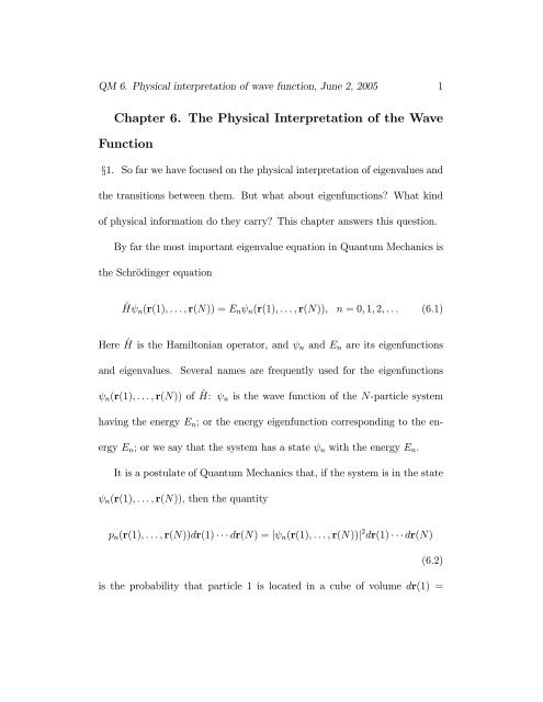
QM <strong>6.</strong> <strong>Physical</strong> interpretation <strong>of</strong> wave function, June 2, 2005 1<br />
<strong>Chapter</strong> <strong>6.</strong> <strong>The</strong> <strong>Physical</strong> <strong>Interpretation</strong> <strong>of</strong> <strong>the</strong> <strong>Wave</strong><br />
<strong>Function</strong><br />
x1. So far we have focused on <strong>the</strong> physical interpretation <strong>of</strong> eigenvalues and<br />
<strong>the</strong> transitions between <strong>the</strong>m. But what about eigenfunctions What kind<br />
<strong>of</strong> physical information do <strong>the</strong>y carry This chapter answers this question.<br />
By far <strong>the</strong> most important eigenvalue equation in Quantum Mechanics is<br />
<strong>the</strong> SchrÄodinger equation<br />
^Hà n (r(1);:::;r(N)) = E n à n (r(1);:::;r(N)); n =0; 1; 2;::: (<strong>6.</strong>1)<br />
Here ^H is <strong>the</strong> Hamiltonian operator, and à n and E n are its eigenfunctions<br />
and eigenvalues. Several names are frequently used for <strong>the</strong> eigenfunctions<br />
à n (r(1);:::;r(N)) <strong>of</strong> ^H: Ãn is <strong>the</strong> wave function <strong>of</strong> <strong>the</strong> N-particle system<br />
having <strong>the</strong> energy E n ; or <strong>the</strong> energy eigenfunction corresponding to <strong>the</strong> energy<br />
E n ; or we say that <strong>the</strong> system has a state à n with <strong>the</strong> energy E n .<br />
It is a postulate <strong>of</strong> Quantum Mechanics that, if <strong>the</strong> system is in <strong>the</strong> state<br />
à n (r(1);:::;r(N)), <strong>the</strong>n <strong>the</strong> quantity<br />
p n (r(1);:::;r(N))dr(1) ¢¢¢dr(N) =jà n (r(1);:::;r(N))j 2 dr(1) ¢¢¢dr(N)<br />
(<strong>6.</strong>2)<br />
is <strong>the</strong> probability that particle 1 is located in a cube <strong>of</strong> volume dr(1) =
QM <strong>6.</strong> <strong>Physical</strong> interpretation <strong>of</strong> wave function, June 2, 2005 2<br />
dx(1)dy(1)dz(1) centered around r(1), and particle 2 is located in a cube <strong>of</strong><br />
volume dr(2) = dx(2)dy(2)dz = (2) centered around r(2), and . . . . In what<br />
follows, jÃj 2 ´ à ¤ à where à ¤ is <strong>the</strong> complex conjugate <strong>of</strong> Ã.<br />
This information is valid only if we are sure that <strong>the</strong> system is in <strong>the</strong><br />
state à n (r(1);:::;r(N)). To be sure <strong>of</strong> that, we must perform an experiment<br />
that places <strong>the</strong> system in that state. For example, we can force a molecule<br />
that is initially in <strong>the</strong> ground state E 0 to absorb a photon and be excited to<br />
<strong>the</strong> state à 2 (r(1);:::;r(N)). <strong>The</strong> probability that <strong>the</strong> atoms in <strong>the</strong> excited<br />
molecule have certain positions r(1);:::;r(N) is given by Eq. <strong>6.</strong>2 with n =2.<br />
I will con¯ne <strong>the</strong> discussion that follows to <strong>the</strong> case <strong>of</strong> a particle moving<br />
along a straight line. I do this to simplify some <strong>of</strong> <strong>the</strong> equations. What you<br />
learn from <strong>the</strong>se examples can be easily extended to many particles moving<br />
in three-dimensional space.<br />
If <strong>the</strong> particle moves along a straight line (one-dimensional motion), its<br />
position is speci¯ed by one coordinate x. If <strong>the</strong> particle is in a state whose<br />
wave function is Ã(x), <strong>the</strong>n <strong>the</strong> probability that <strong>the</strong> particle is located between<br />
x and x + dx is<br />
p(x)dx = jÃ(x)j 2 dx (<strong>6.</strong>3)<br />
<strong>The</strong> probability that <strong>the</strong> particle is located in <strong>the</strong> region between a and
QM <strong>6.</strong> <strong>Physical</strong> interpretation <strong>of</strong> wave function, June 2, 2005 3<br />
b is <strong>the</strong>n<br />
Z b<br />
a<br />
p(x)dx =<br />
Z b<br />
a<br />
jÃ(x)j 2 dx (<strong>6.</strong>4)<br />
We add up <strong>the</strong> probabilities that <strong>the</strong> particle is at points between a and b.<br />
<strong>The</strong> probability that <strong>the</strong> particle is somewhere along <strong>the</strong> line is<br />
Z +1<br />
¡1<br />
jÃ(x)j 2 dx =1 (<strong>6.</strong>5)<br />
This integral is equal to 1 because we are certain that <strong>the</strong> particle is somewhere<br />
on <strong>the</strong> line; <strong>the</strong> probability <strong>of</strong> an event that is certain is equal to 1, by<br />
de¯nition.<br />
When a wave function satis¯es Eq. <strong>6.</strong>5, we say that it is normalized.<br />
Eq. <strong>6.</strong>5 is called <strong>the</strong> normalization condition. We can generalize this condition<br />
to <strong>the</strong> case <strong>of</strong> N particles moving in three-dimensional space:<br />
Z +1<br />
¡1<br />
jÃ(r(1); r(2);:::;r(N))j 2 dr(1)dr(2) ¢¢¢dr(N) =1<br />
<strong>The</strong> probability that <strong>the</strong> N particles are somewhere in <strong>the</strong> space must be<br />
equal to 1.<br />
It is this interpretation <strong>of</strong> <strong>the</strong> wave function that prompted us to require<br />
that all eigenstates that have a physical meaning must be normalized.<br />
x2. Application to a vibrating diatomic molecule. To better understand <strong>the</strong><br />
probabilistic interpretation <strong>of</strong> <strong>the</strong> wave function and <strong>the</strong> manner in which it
QM <strong>6.</strong> <strong>Physical</strong> interpretation <strong>of</strong> wave function, June 2, 2005 4<br />
A<br />
B<br />
Figure <strong>6.</strong>1: A model for a vibrating diatomic molecule: two atoms connected<br />
by a spring<br />
is used, I will examine <strong>the</strong> example <strong>of</strong> a vibrating molecule. <strong>The</strong> simplest<br />
model for <strong>the</strong> vibrational motion <strong>of</strong> a diatomic molecule assumes that <strong>the</strong><br />
interaction between <strong>the</strong> two atoms is accurately simulated by a spring (see<br />
Fig. <strong>6.</strong>1). <strong>The</strong> potential energy <strong>of</strong> such a spring is<br />
V (x) = 1 2 k (r ¡ r 0) 2 ´ kx2<br />
2<br />
(<strong>6.</strong>6)<br />
where r is <strong>the</strong> distance between <strong>the</strong> centers <strong>of</strong> <strong>the</strong> atoms and k is called <strong>the</strong><br />
force constant <strong>of</strong> <strong>the</strong> bond (<strong>the</strong> spring). <strong>The</strong> distance r 0 corresponds to <strong>the</strong><br />
lowest potential energy, and it is <strong>the</strong> bond length. It is not di±cult to show<br />
that <strong>the</strong> potential energy V (x) in Eq. <strong>6.</strong>6 leads, in classical mechanics, to an<br />
oscillatory motion <strong>of</strong> <strong>the</strong> distance x between <strong>the</strong> atoms, with a frequency<br />
s<br />
k<br />
! =<br />
¹
QM <strong>6.</strong> <strong>Physical</strong> interpretation <strong>of</strong> wave function, June 2, 2005 5<br />
where<br />
¹ = m 1m 2<br />
m 1 + m 2<br />
is <strong>the</strong> e®ective mass (m 1 and m 2 are <strong>the</strong> masses <strong>of</strong> <strong>the</strong> two atoms).<br />
Since we know <strong>the</strong> potential energy, we can write <strong>the</strong> SchrÄodinger equation<br />
for this system and solve it. For <strong>the</strong> ground state (<strong>the</strong> lowest energy<br />
eigenstate), <strong>the</strong> wave function is<br />
à 0 (x) =<br />
µ #<br />
¹!<br />
1=4<br />
exp<br />
"¡ ¹!x2<br />
¼¹h<br />
2¹h<br />
(<strong>6.</strong>7)<br />
and <strong>the</strong> ground state energy is<br />
E 0 = ¹h! 2<br />
(<strong>6.</strong>8)<br />
<strong>The</strong>wavefunction<strong>of</strong><strong>the</strong>¯rstexcitedstateis<br />
with <strong>the</strong> energy<br />
Ã<br />
4<br />
à 1 (x) =<br />
¼<br />
µ !<br />
¹!<br />
3 1=4 ∙<br />
x exp ¡ ¹!<br />
x2¸<br />
¹h<br />
2¹h<br />
E 1 = 3¹h!<br />
2<br />
(<strong>6.</strong>9)<br />
(<strong>6.</strong>10)<br />
We will study harmonic oscillators in more detail in <strong>Chapter</strong> 1<strong>6.</strong> <strong>The</strong><br />
information given above is all we need here.<br />
x3. Data for HCl. To perform calculations with <strong>the</strong> wave functions given<br />
above, we need to work with a speci¯c molecule. I choose here HCl, for which<br />
I have <strong>the</strong> following data.
QM <strong>6.</strong> <strong>Physical</strong> interpretation <strong>of</strong> wave function, June 2, 2005 6<br />
<strong>The</strong> reduced mass is ¹ = m 1 m 2 =(m 1 + m 2 ). For m 1 =1:0078 amu =<br />
1:0078 £ 1:6605 £ 10 ¡24 gram and m 2 =34:968 amu = 34:968 £ 1:6605 £<br />
10 ¡24 gram (I use <strong>the</strong> conversion factor 1 amu = 1:6605£10 ¡24 g; see Appendix<br />
1), I have ¹ =0:979568 £ 1:6605 £ 10 ¡24 gram (see WorkBookQM.<strong>6.</strong>1).<br />
Since <strong>the</strong> force constant 1 is k =4:9 £ 10 5 dyne/cm, we calculate that <strong>the</strong><br />
frequency ! has <strong>the</strong> value<br />
s s<br />
k<br />
! =<br />
¹ = 4:9 £ 10 5 erg<br />
0:979568 £ 1:6605 £ 10 ¡24 gr =5:4886 £ 1014 sec ¡1<br />
Using ¹h =1:0546 £ 10 ¡27 erg sec (see Appendix 1) and <strong>the</strong> values <strong>of</strong> ¹<br />
and ! just calculated, we can write<br />
à 0 (x) =<br />
Ã<br />
0:979 £ 1:66 £ 10 ¡24 £ 5:489 £ 10 14<br />
£ exp<br />
"<br />
¼ £ 1:055 £ 10 ¡27<br />
! 1=4<br />
g<br />
sec erg sec<br />
¡ 0:979 £ 1:66 £ 10¡24 £ 5:489 £ 10 14 gcm 2<br />
2 £ 1:055 £ 10 ¡27 sec erg sec<br />
µ #<br />
x<br />
2<br />
cm<br />
(<strong>6.</strong>11)<br />
Let us look at units. <strong>The</strong> unit <strong>of</strong> <strong>the</strong> wave function is (g/erg sec 2 ) 1=4 ,<br />
where g stands for grams. Since erg = g cm 2 sec ¡2 ,wehave<br />
g<br />
sec 2 erg =<br />
g<br />
= 1<br />
sec 2 g cm2 cm ; 2 sec 2<br />
1 D. A. McQuarrie, Statistical Mechanics, Harper Collins, New York, 1976, p. 95
QM <strong>6.</strong> <strong>Physical</strong> interpretation <strong>of</strong> wave function, June 2, 2005 7<br />
and <strong>the</strong> wave function has units <strong>of</strong><br />
"<br />
gr<br />
# 1=4<br />
= 1<br />
sec 2 erg cm 1=2<br />
But cm is a cumbersome unit for length in molecular physics, because it is<br />
much too large. I will use ºA instead. This means that<br />
"<br />
# 1=4<br />
g<br />
= 1<br />
sec 2 erg cm = 1<br />
1=2<br />
10 4 ºA 1=2<br />
and <strong>the</strong> factor in front <strong>of</strong> <strong>the</strong> exponential in Eq. <strong>6.</strong>11 is<br />
Ã<br />
0:979 £ 1:66 £ 10 ¡24 £ 5:489 £ 10 14 ! 1=4<br />
1 2:27837<br />
= (<strong>6.</strong>12)<br />
¼ £ 1:055 £ 10 ¡27 10 4 1=2<br />
ºA ºA 1=2<br />
<strong>The</strong> units <strong>of</strong> <strong>the</strong> exponent in Eq. <strong>6.</strong>11 are<br />
gcm 2<br />
sec 2 erg =1<br />
This means that <strong>the</strong> exponent is dimensionless, if I use for x units <strong>of</strong> cm.<br />
But I want to use ºA. <strong>The</strong>refore <strong>the</strong> exponent is<br />
¡ 0:979 £ 1:66 £ 10¡24 £ 5:489 £ 10 14 µ x 2 µ x 2<br />
= ¡42:327 (<strong>6.</strong>13)<br />
2 £ 1:055 £ 10 ¡27 10 ºA 8 ºA<br />
In this expression I must use x in ºA.<br />
Putting it all toge<strong>the</strong>r gives<br />
à 0 (x) = 2:27837<br />
" µ #<br />
x<br />
2<br />
exp ¡42:327<br />
ºA<br />
ºA 1=2<br />
(<strong>6.</strong>14)
QM <strong>6.</strong> <strong>Physical</strong> interpretation <strong>of</strong> wave function, June 2, 2005 8<br />
<strong>The</strong> probability that <strong>the</strong> di®erence x = r ¡ r 0 , between <strong>the</strong> interatomic<br />
distance r and <strong>the</strong> equilibrium bond length r 0 ,takesavaluebetweenx and<br />
x + dx, when <strong>the</strong> vibrating molecule is in <strong>the</strong> ground state (see x1), is<br />
p 0 (x)dx =<br />
à " µ #!<br />
2:27837<br />
x<br />
2 2<br />
exp ¡42:327 dx (<strong>6.</strong>15)<br />
ºA 1=2 ºA<br />
Because <strong>the</strong> wave function has units <strong>of</strong> ºA ¡1=2 , dx in this formula must have<br />
units <strong>of</strong> ºA andp(x)dx is dimensionless (as it should be).<br />
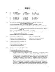
A plot <strong>of</strong> <strong>the</strong> probability distribution function p 0 (x) versusx is shown<br />
in Fig. <strong>6.</strong>2 as a solid line.<br />
As you can see, when <strong>the</strong> molecule is in <strong>the</strong><br />
ground state, it is more likely that <strong>the</strong> distance between <strong>the</strong> atoms is equal<br />
to <strong>the</strong> equilibrium distance r 0 . However, <strong>the</strong> probability that <strong>the</strong> bond length<br />
deviates from this value (i.e. that x = r ¡ r 0 6= 0) is not negligible.<br />
<strong>The</strong> ¯gure also shows (dotted line) <strong>the</strong> probability distribution function<br />
p 1 (x) =à 1 (x) ¤ à 1 (x) ´jà 1 (x)j 2<br />
when <strong>the</strong> molecule is excited in <strong>the</strong> ¯rst vibrational state. Here à 1 is given<br />
by Eq. <strong>6.</strong>9. p 1 (x)dx is <strong>the</strong> probability that r ¡ r 0 takesvaluesbetweenx and<br />
x + dx, when we know that <strong>the</strong> oscillator is excited to <strong>the</strong> state à 1 .<br />
x4. <strong>Interpretation</strong>. Here we go again: probabilities instead <strong>of</strong> certainty. <strong>The</strong><br />
laws <strong>of</strong> classical mechanics place no restrictions, in principle, on position
QM <strong>6.</strong> <strong>Physical</strong> interpretation <strong>of</strong> wave function, June 2, 2005 9<br />
5<br />
|ψ 0 | 2<br />
4<br />
3<br />
2<br />
|ψ 1 | 2<br />
1<br />
-0.4 -0.2 0.2 0.4<br />
x=r 12 -r 0 Angstrom<br />
Figure <strong>6.</strong>2: Probability distributions for <strong>the</strong> bond length x when <strong>the</strong> oscillator<br />
is in <strong>the</strong> ground state (solid line) and <strong>the</strong> ¯rst excited state (dashed line)<br />
measurements.<br />
Only technical di±culties prevent us from measuring <strong>the</strong><br />
position with arbitrary accuracy.<br />
Quantum Mechanics tells us that if we<br />
were to measure <strong>the</strong> interatomic distance r, for a single oscillator, we would<br />
get di®erent results in di®erent measurements, performed under identical<br />
conditions.<br />
As in <strong>the</strong> case <strong>of</strong> <strong>the</strong> measurements discussed in <strong>the</strong> previous chapter,<br />
knowing <strong>the</strong> probability with which something takes place is useful when we<br />
make a large number N <strong>of</strong> identical measurements. If N is large enough, we
QM <strong>6.</strong> <strong>Physical</strong> interpretation <strong>of</strong> wave function, June 2, 2005 10<br />
can be sure that for<br />
Np 0 (x)dx<br />
oscillators in <strong>the</strong> ground state à 0 (x), x ´ r ¡ r 0 takesvaluesbetweenx and<br />
x + dx.<br />
x5. Average values. <strong>The</strong> probability is also useful for calculating various<br />
averages. For example, <strong>the</strong> average distance between <strong>the</strong> atoms, when <strong>the</strong><br />
diatomic molecule is in <strong>the</strong> ground state, is<br />
hri =<br />
Z 1<br />
¡1<br />
= r 0<br />
Z 1<br />
= r 0<br />
rp 0 (r)dr =<br />
¡1<br />
p 0 (x)dx +<br />
Z 1<br />
¡1<br />
Z 1<br />
¡1<br />
(r 0 + x) p 0 (x)dx<br />
xp 0 (x)dx<br />
In this calculation we have used <strong>the</strong> fact that x = r ¡ r 0 and<br />
p 0 (r)dr = p 0 (x)dx<br />
Here p 0 (r)dr is <strong>the</strong> probability that <strong>the</strong> distance between <strong>the</strong> atoms takes<br />
values between r and r + dr when <strong>the</strong> molecule is in <strong>the</strong> ground state. We<br />
have also used <strong>the</strong> facts that<br />
and<br />
Z 1<br />
¡1<br />
Z 1<br />
¡1<br />
p 0 (r)dr =1<br />
xp 0 (x)dx =0
QM <strong>6.</strong> <strong>Physical</strong> interpretation <strong>of</strong> wave function, June 2, 2005 11<br />
You can calculate <strong>the</strong>se integrals fairly easily by hand, or by Ma<strong>the</strong>matica<br />
or Mathcad.<br />
Exercise <strong>6.</strong>1 You have a sample <strong>of</strong> 10 12 HCl molecules. <strong>The</strong> force constant<br />
is k =4:9 £ 10 5 dyne/cm and <strong>the</strong> equilibrium bond length is r 0 =1:27460<br />
ºA. Calculate how many molecules that are in <strong>the</strong> ground state have a bond<br />
length between 1.24 ºA and1.29ºA.<br />
Exercise <strong>6.</strong>2 Do <strong>the</strong> same type <strong>of</strong> calculation for I 2 .<br />
For this molecule,<br />
r 0 =2:666 ºA and! =214:57 cm ¡1 . (Data from G. Herzberg, Molecular<br />
Spectra and Molecular Structure. I. Spectra <strong>of</strong> Diatomic Molecules, VanNostrand,<br />
New York, 1950, p. 540.) Calculate how many molecules, out <strong>of</strong> 10 12 ,<br />
have an interatomic distance between 2.53 ºA and2.66ºA.<br />
Note: ! =214:57 cm ¡1 is a strange unit.<br />
In Appendix 2, <strong>the</strong>re is a table<br />
that tells you that 1 cm ¡1 = 1:9862 £ 10 ¡16 erg. This means that<br />
¹h! = 1:9862 £ 10 ¡16 £ 214:57 erg.<br />
From this information, I can calculate<br />
<strong>the</strong> frequency: since ¹h =1:0546 £ 10 ¡27 erg sec, I have ! =¹h!=¹h =<br />
(1:9862 £ 10 ¡16 £ 214:57) = (1:0546 £ 10 ¡27 )=4:041 £ 10 13 sec ¡1 .<br />
x<strong>6.</strong> <strong>The</strong> e®ect <strong>of</strong> position uncertainty on a di®raction experiment. Let us look<br />
at a system consisting <strong>of</strong> diatomic molecules adsorbed on a surface. Under
QM <strong>6.</strong> <strong>Physical</strong> interpretation <strong>of</strong> wave function, June 2, 2005 12<br />
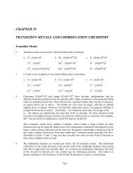
(a)<br />
(b)<br />
Figure <strong>6.</strong>3: Upper ¯gure shows <strong>the</strong> surface atoms undisturbed by uncertainty<br />
in positions. Lower one shows <strong>the</strong> real instantaneous positions.<br />
certain conditions, <strong>the</strong>se molecules position <strong>the</strong>mselves to form a periodic<br />
array (see Fig. <strong>6.</strong>3). If all <strong>the</strong> molecules have <strong>the</strong> same bond length, <strong>the</strong>y form<br />
a perfect \grating" on <strong>the</strong> surface (Fig. <strong>6.</strong>3a). If we scatter from <strong>the</strong> surface<br />
a beam <strong>of</strong> X-rays (or electrons) having a certain wavelength, <strong>the</strong> grating will<br />
di®ract <strong>the</strong> beam and produce a di®raction pattern. From this pattern, we<br />
can, by using di®raction <strong>the</strong>ory, determine <strong>the</strong> positions <strong>of</strong> atoms.<br />
However, we know that <strong>the</strong> molecules will not have <strong>the</strong> same bond length.<br />
AccordingtoQuantumMechanics,<strong>the</strong>bondlengthineachmoleculehasa<br />
given value with a given probability.<br />
<strong>The</strong> instantaneous positions <strong>of</strong> <strong>the</strong>
QM <strong>6.</strong> <strong>Physical</strong> interpretation <strong>of</strong> wave function, June 2, 2005 13<br />
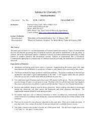
Figure <strong>6.</strong>4: <strong>The</strong> dotted lines show <strong>the</strong> locations <strong>the</strong> atom can reach due to<br />
uncertainty in position<br />
atoms are shown, with some exaggeration, in Fig. <strong>6.</strong>3b. <strong>The</strong> grating formed<br />
by <strong>the</strong> molecules is not perfect.<br />
We can calculate <strong>the</strong> di®raction pattern<br />
produced by <strong>the</strong> molecules in Fig. <strong>6.</strong>3a and by those in Fig. <strong>6.</strong>3b. When calculating<br />
<strong>the</strong> di®raction pattern produced by Fig. <strong>6.</strong>3b, we use <strong>the</strong> probability<br />
p 0 (x)dx. <strong>The</strong> experiments ¯nd that <strong>the</strong> observed pattern is that calculated<br />
for <strong>the</strong> imperfect grating. This is an indirect con¯rmation <strong>of</strong> <strong>the</strong> quantum mechanical<br />
postulate that di®erent distances between atoms are observed with<br />
di®erent probabilities; moreover, <strong>the</strong> agreement with experiment is quantitative,<br />
con¯rming <strong>the</strong> formula used for computing <strong>the</strong> probability that <strong>the</strong><br />
molecule has a given <strong>the</strong> bond length.<br />
x7. <strong>The</strong> e®ect <strong>of</strong> position uncertainty in an ESDAID experiment. Consider
QM <strong>6.</strong> <strong>Physical</strong> interpretation <strong>of</strong> wave function, June 2, 2005 14<br />
ano<strong>the</strong>r experiment, performed by John Yates and Ted Madey, when <strong>the</strong>y<br />
were working at NIST. <strong>The</strong>y started with a perfect metal surface whose<br />
atoms are arranged in a nearly perfect periodic array (see Fig. <strong>6.</strong>4). <strong>The</strong>n<br />
<strong>the</strong>y adsorbed atoms or molecules on <strong>the</strong> surface. In Fig. <strong>6.</strong>4, I show one such<br />
atom, adsorbed on top <strong>of</strong> a surface atom. <strong>The</strong> most likely position <strong>of</strong> <strong>the</strong><br />
adsorbed atom is shown by heavy lines in Fig. <strong>6.</strong>4. However, <strong>the</strong> positions<br />
shown with dotted lines | and those between <strong>the</strong>m| also occur with some<br />
probability.<br />
This surface is bombarded with high-energy electrons, which break <strong>the</strong><br />
metal-atom chemical bond. When <strong>the</strong> bond is broken <strong>the</strong> adsorbed atoms<br />
come o® <strong>the</strong> surface. <strong>The</strong> atoms whose bond is perpendicular to <strong>the</strong> surface<br />
leave it, when <strong>the</strong> bond is broken, in a direction perpendicular to <strong>the</strong> surface<br />
(see <strong>the</strong> solid line and arrow in <strong>the</strong> ¯gure). <strong>The</strong> ones that are slanted come<br />
o®, when <strong>the</strong> bond is broken, at an angle with <strong>the</strong> surface. <strong>The</strong> experiment<br />
detects <strong>the</strong> point where <strong>the</strong> atoms leaving <strong>the</strong> surface hit a position-sensitive<br />
detector (represented by a slab at <strong>the</strong> top <strong>of</strong> <strong>the</strong> ¯gure). An atom that leaves<br />
<strong>the</strong> surface on a trajectory perpendicular to <strong>the</strong> surface hits <strong>the</strong> center <strong>of</strong> <strong>the</strong><br />
detector. One that leaves <strong>the</strong> surface on a slanted trajectory hits <strong>the</strong> detector<br />
o®-center. From <strong>the</strong> distribution <strong>of</strong> <strong>the</strong> points <strong>of</strong> impact on <strong>the</strong> detector, one
QM <strong>6.</strong> <strong>Physical</strong> interpretation <strong>of</strong> wave function, June 2, 2005 15<br />
can calculate <strong>the</strong> probability <strong>of</strong> <strong>the</strong> initial position <strong>of</strong> <strong>the</strong> atom. <strong>The</strong> result<br />
agrees with Quantum Mechanical calculations.<br />
I should caution you that <strong>the</strong> real experiment is close in spirit to <strong>the</strong><br />
description just given, but is more complicated.<br />
x8. Why did we think that we could measure position accurately You have<br />
just learned that we cannot know with certainty <strong>the</strong> positions <strong>of</strong> <strong>the</strong> particles<br />
in a system. Why isn't this true for <strong>the</strong> large objects we encounter in everyday<br />
life Quantum mechanics has a simple answer: <strong>the</strong> larger a particle, <strong>the</strong> less<br />
uncertain its position.<br />
Let us see how we reach this conclusion, in <strong>the</strong> case <strong>of</strong> <strong>the</strong> bond length<br />
<strong>of</strong> a vibrating diatomic molecule. If <strong>the</strong> oscillator is in <strong>the</strong> ground state, <strong>the</strong><br />
probability that x = r ¡ r 0 has a value between x and x + dx is<br />
I can write Eq. <strong>6.</strong>16 as<br />
jà 0 (x)j 2 dx =<br />
jà 0 (x)j 2 dx =<br />
µ #<br />
¹!<br />
1=2<br />
exp<br />
"¡ ¹!x2 dx (<strong>6.</strong>16)<br />
¼¹h<br />
¹h<br />
µ 1 1=2<br />
" µ #<br />
x<br />
2<br />
exp ¡ dx (<strong>6.</strong>17)<br />
¼¾ 2 ¾<br />
where<br />
¾ 2 ´ ¹h<br />
¹!<br />
(<strong>6.</strong>18)<br />
is a quantity with units <strong>of</strong> length squared.
QM <strong>6.</strong> <strong>Physical</strong> interpretation <strong>of</strong> wave function, June 2, 2005 16<br />
From Eq. <strong>6.</strong>18 you can see that if x À ¾, <strong>the</strong>njà 0 (x)j 2 is practically zero.<br />
<strong>The</strong>refore I am sure that <strong>the</strong> bond length r is never much longer than r 0 + ¾,<br />
nor is it much shorter than r 0 ¡ ¾. <strong>The</strong>smaller¾ is, <strong>the</strong> more accurate is my<br />
knowledge <strong>of</strong> <strong>the</strong> bond length. Thus ¾ is a good descriptor <strong>of</strong> <strong>the</strong> accuracy<br />
with which I can know <strong>the</strong> bond length.<br />
Let us calculate ¾ for a diatomic whose reduced mass is a gram and whose<br />
frequency is ! =10 14 sec ¡1 .Inthiscase<br />
¾ 2 = ¹h<br />
¹! = 1:0546 £ 10¡27 erg sec<br />
1gr£ 10 14 gr/sec<br />
I¯ndthat¾ 2 » = 10 ¡41 cm 2 and ¾ » = p 10 £ 10 ¡20 cm.<br />
This uncertainty in position is beyond <strong>the</strong> accuracy <strong>of</strong> any conceivable instrument.<br />
Because <strong>of</strong> this, in <strong>the</strong> classical world (large mass), we are entitled<br />
to claim that it is possible to know <strong>the</strong> position <strong>of</strong> a particle with \unlimited"<br />
accuracy. We know that this is not quite right, but no one will be able to<br />
prove us wrong in our lifetime.<br />
<strong>The</strong> statement that position is precisely known when <strong>the</strong> mass is large is a<br />
dumb statement, even though it is made frequently. <strong>The</strong> word `large' makes<br />
sense only if we compare one mass to ano<strong>the</strong>r. When I say that a friend is<br />
heavy, I am implicitly compare him to <strong>the</strong> average person, or compare his<br />
weight to what it was twenty years ago. So what do I mean when I say that
QM <strong>6.</strong> <strong>Physical</strong> interpretation <strong>of</strong> wave function, June 2, 2005 17<br />
for a heavy oscillator, <strong>the</strong> position is known accurately Heavy compared to<br />
what<br />
This is easy to answer for <strong>the</strong> case <strong>of</strong> <strong>the</strong> oscillator. Let us say that <strong>the</strong><br />
highest accuracy <strong>of</strong> <strong>the</strong> best position measurement is ¾ 0 .If<br />
s<br />
¹h<br />
¹! ¿ ¾ 0 (<strong>6.</strong>19)<br />
<strong>the</strong>n <strong>the</strong> quantum uncertainty in <strong>the</strong> position <strong>of</strong> <strong>the</strong> oscillator is not detectable.<br />
<strong>The</strong> inequality (<strong>6.</strong>19) is satis¯ed if <strong>the</strong> mass satis¯es<br />
s<br />
¹h<br />
¹ À<br />
!¾ 2 0<br />
If ¾ 0 =10 ¡8 cm, <strong>the</strong>n<br />
s<br />
1:0546 £ 10<br />
¡27<br />
¹><br />
g= p 10<br />
10 14 £ 10 ¡25 g= p 10 £ 10 ¡12 g<br />
¡16<br />
For a diatomic with reduced mass exceeding 3 £ 10 ¡12 gram, <strong>the</strong> di®erence<br />
in <strong>the</strong> bond length between di®erent copies <strong>of</strong> <strong>the</strong> same molecule is not detectable.<br />
Because classical physics deals with objects heavier than 10 ¡12<br />
gram, we can claim that position is accurately determined by <strong>the</strong> laws <strong>of</strong><br />
mechanics.<br />
Exercise <strong>6.</strong>3 One way <strong>of</strong> describing <strong>the</strong> uncertainty in <strong>the</strong> position is to use<br />
<strong>the</strong> mean-square error<br />
Z +1<br />
`2 ´<br />
¡1<br />
x 2 jà 0 (x)j 2 dx
QM <strong>6.</strong> <strong>Physical</strong> interpretation <strong>of</strong> wave function, June 2, 2005 18<br />
Calculate this quantity and show that ` is <strong>of</strong> order ¾ = q ¹h=¹!.