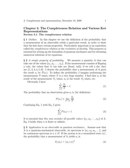
Chapter 3. The Completeness Relation and Various Ket ...
Chapter 3. The Completeness Relation and Various Ket ...
Chapter 3. The Completeness Relation and Various Ket ...

You also want an ePaper? Increase the reach of your titles
YUMPU automatically turns print PDFs into web optimized ePapers that Google loves.
<strong>3.</strong> <strong>Completeness</strong> <strong>and</strong> representations, December 10, 2009 1<br />
<strong>Chapter</strong> <strong>3.</strong> <strong>The</strong> <strong>Completeness</strong> <strong>Relation</strong> <strong>and</strong> <strong>Various</strong> <strong>Ket</strong><br />
Representations<br />
Section <strong>3.</strong>1. <strong>The</strong> completeness relation<br />
§ 1 Outline. In this chapter we use the definition of the probability that<br />
a measurement of an observable yields a particular result, in order to show<br />
that the kets have certain properties. Particularly important is an expression<br />
called the completeness relation or the resolution of identity. Thispropertyis<br />
essential for setting up the formalism of quantum mechanics <strong>and</strong> for obtaining<br />
numerical solutions of its equations.<br />
§ 2 A simple property of probability. We measure a quantity A that can<br />
take one of the values {a 1 ,a 2 ,...,a n }. If the measurement consists of flipping<br />
a coin, the values that A can take are {head, tail}; ifwerolladie,they<br />
are {1, 2, 3, 4, 5, 6}. I denote the probability that a measurement of A gives<br />
the result a i by P (a i ). To define the probability, I imagine performing the<br />
measurement N times, where N is a very large number. I find that a 1 is the<br />
result of the measurement N 1 times, a 2 is the result N 2 times, etc.<br />
Obviously I have<br />
n N i<br />
=1 (1)<br />
i=1<br />
N<br />
<strong>The</strong> probability that an observation gives a i is (by definition)<br />
N i<br />
P (a i ) ≡ lim<br />
N→∞ N<br />
Combining Eq. 1 with Eq. 2 gives<br />
(2)<br />
n<br />
P (a i )=1 (3)<br />
i=1<br />
It is essential that this sum includes all possible values {a 1 ,a 2 ,...,a n } of A.<br />
Eq. 3 holds when n is finite or infinite.<br />
§ 3 Application to an observable in quantum mechanics. Assume now that<br />
A is a quantum-mechanical observable, its spectrum is {a 1 ,a 2 ,a 3 ,...}, <strong>and</strong><br />
its continuous spectrum is α ∈ D. If the system is in a normalized state |ψ,<br />
the probability that a measurement of A yields a i is<br />
P ψ (a i )=|a i | ψ| 2 (4)
<strong>3.</strong> <strong>Completeness</strong> <strong>and</strong> representations, December 10, 2009 2<br />
<strong>The</strong> probability that the result of the measurement is a value between α <strong>and</strong><br />
α +dα is<br />
P ψ (α)dα = |α | ψ| 2 dα, α ∈ D (5)<br />
By definition, the spectrum contains all values that A can take <strong>and</strong> so Eq. 3<br />
applies for these probabilities:<br />
∞<br />
<br />
P ψ (a i )+<br />
i=1<br />
α∈D<br />
dα P ψ (α) =<br />
∞<br />
<br />
|a i | ψ| 2 +<br />
i=1<br />
α∈D<br />
dα |α | ψ| 2 =1 (6)<br />
We have generalized Eq. 3 to include the continuous spectrum by using an<br />
integral instead of a sum.<br />
§ 4 Dirac notation: operators <strong>and</strong> bras. For any complex number z, we<br />
have |z| 2 = z ∗ z; for any scalar product, λ | μ = μ | λ ∗ . Combining these<br />
two equations gives |a i | ψ| 2 = ψ | a i a i | ψ. Using this result we rewrite<br />
Eq. 6 as<br />
∞<br />
<br />
ψ | a n a n | ψ + dα ψ | αα | ψ =1 (7)<br />
n=1<br />
α∈D<br />
At this point we follow Dirac <strong>and</strong> introduce a very innovative <strong>and</strong> useful<br />
notation:<br />
ψ | a n a n | ψ ≡ψ | (|a n a n |) | ψ (8)<br />
This is an identity in which the left-h<strong>and</strong> side is written (in the righth<strong>and</strong><br />
side) as a product of three distinct symbols: the bra ψ|, theoperator<br />
|a n a n |,<strong>and</strong>theket|ψ.<br />
We already know what a ket is; but the bra <strong>and</strong> the operator are new<br />
objects, defined by Eq. 8. Let us take a look at what they do.<br />
Abraa| must be understood as a symbol that acts on a ket; the rule<br />
for this action is (a|)|ψ = a | ψ. A bra a| acting on a ket |ψ gives the<br />
complex number a | ψ. For every ket |η, in a given ket space, there is a<br />
corresponding bra η| defined by the rule given above, <strong>and</strong> vice versa. Thus<br />
the bras form a space of their own <strong>and</strong> there is a one-to-one correspondence<br />
between the bra space <strong>and</strong> the ket space.<br />
<strong>The</strong> manner in which bras are defined allows us to derive rules of computation<br />
for them. If |λ = |η + |μ then we can use the properties of the<br />
scalar product to write<br />
λ | ψ = ψ | λ ∗ = ψ | η ∗ + ψ | μ ∗ = η | ψ + μ | ψ (9)
<strong>3.</strong> <strong>Completeness</strong> <strong>and</strong> representations, December 10, 2009 3<br />
<strong>The</strong>reforewehavetherule:<br />
if |λ = |η + |μ then λ| = η| + μ| (10)<br />
Similarly, if |η = α|a, whereα is a complex number, then<br />
η | ψ = ψ | η ∗ = ψ | αa ∗ =(αψ | a) ∗ = α ∗ a | ψ (11)<br />
<strong>and</strong> therefore, we have the rule:<br />
if |η = α|a then η| = α ∗ a| (12)<br />
<strong>The</strong> operator<br />
ˆP (a n ) ≡ |a n a n | (13)<br />
is also a new mathematical object. By definition it acts on a ket |ψ through<br />
the rule<br />
ˆP (a n )|ψ =(|a n a n |)|ψ = |a n a n | ψ (14)<br />
An operator (here, |a n a n |)actsonaket(here,|ψ) to produce another ket<br />
(here, |a n a n | ψ). <strong>The</strong> product |a n a n | ψ is a ket because a n | ψ is a<br />
complex number, |a n is a ket, <strong>and</strong> the product of a complex number <strong>and</strong> a<br />
ket is a ket. An operator is any object that acts on a ket to generate another<br />
ket.<br />
§ 5 <strong>The</strong> completeness relation. Now that we are comfortable with Dirac’s<br />
notation, let us use it to rewrite Eq. 7 as<br />
∞<br />
<br />
ψ | ( |a n a n | + dα |αα|) | ψ =1 (15)<br />
n=1<br />
α∈D<br />
This is equivalent to setting<br />
∞<br />
<br />
|a n a n | +<br />
n=1<br />
α∈D<br />
dα |αα| = Î (16)<br />
where Î is the unit operator, defined to give<br />
Î|ψ = |ψ for any ket |ψ (17)<br />
It is not difficult to show that Eqs. 16 <strong>and</strong> 17 are equivalent to Eq. 15 (remember<br />
that ψ | ψ =1).
<strong>3.</strong> <strong>Completeness</strong> <strong>and</strong> representations, December 10, 2009 4<br />
Eq. 16 is called the completeness relation for the pure states |a n , n =<br />
1, 2,...,<strong>and</strong>|α, α ∈ D. This is a very complicated way of writing the<br />
operator Î, whoseeffectistodonothing! <strong>The</strong>“derivation”givenaboveis<br />
not rigorous, <strong>and</strong> the result must be used with great care. We are going to<br />
use it often <strong>and</strong> I will point out, at the appropriate places, how easy it is to<br />
misinterpret <strong>and</strong> misuse it.<br />
§ 6 <strong>Completeness</strong> is valid, in principle, for the states of any observable. <strong>The</strong><br />
arguments made in deriving the completeness relation put no constraints<br />
on the observable A; this relationship is valid for the pure states of any<br />
observable.<br />
Let us take as observable the position X of the particle. <strong>The</strong> position has<br />
a continuous spectrum, which contains all real numbers between −∞ <strong>and</strong><br />
+∞. Let |x denote the pure state in which we know for certain that the<br />
value of X is x. <strong>The</strong> completeness relation for these pure states is<br />
Î =<br />
+∞<br />
−∞<br />
dx |xx| (18)<br />
We say that this equation gives the unit operator in the coordinate representation.<br />
<strong>The</strong>re is noting special about coordinates <strong>and</strong> we can play the same game<br />
with the pure states |p of momentum. We have<br />
Î =<br />
+∞<br />
−∞<br />
dp |pp| (19)<br />
because momentum is an observable with a purely continuous spectrum.<br />
Eq. 19 gives the unit operator in the momentum representation.<br />
Finally, the unit operator in the energy representation is<br />
∞<br />
Î = |E n E n | +<br />
n=1<br />
∞<br />
0<br />
dα |E α E α | (20)<br />
where |E n <strong>and</strong> |E α are the pure states of energy.<br />
Section <strong>3.</strong>2. Representation theory<br />
§ 7 <strong>Various</strong> representations of a state |ψ. In many experiments in quantum<br />
mechanics, we force the system (a molecule, a solid, etc.) to interact
<strong>3.</strong> <strong>Completeness</strong> <strong>and</strong> representations, December 10, 2009 5<br />
with an external agent (light, an electron beam, etc.). When this interaction<br />
stops, the system is left in a state |ψ. Quantum theory is then used<br />
to calculate the properties of the system in this state: the probability that<br />
the system has the energy E n , or the average position of the particles in the<br />
system, the evolution of the state in time, etc.<br />
Most of these calculations start by representing |ψ in a convenient form.<br />
One class of representations is generated by starting with the identity<br />
|ψ = Î|ψ (21)<br />
If A is an observable with the discrete spectrum {a n } ∞ n=1 <strong>and</strong> the continuous<br />
spectrum α ∈ D, we can write<br />
Î =<br />
∞<br />
<br />
|a n a n | +<br />
n=1<br />
α∈D<br />
Using this in |ψ = Î|ψ (i.e. Eq. 21), we obtain<br />
|ψ =<br />
∞<br />
<br />
|a n a n | ψ +<br />
n=1<br />
α∈D<br />
|αα| dα (22)<br />
|αα | ψ dα (23)<br />
Here |a n <strong>and</strong> |α are the pure states of the observable A. <strong>The</strong> coefficients<br />
a n | ψ are complex numbers <strong>and</strong> P ψ (a n )=|a n | ψ| 2 is the probability that<br />
a measurement of A, when the system is in the state |ψ, yields the value a n .<br />
α | ψ are also complex numbers <strong>and</strong> P ψ (α) =|α | ψ| 2 dα is the probability<br />
that A takes values between α <strong>and</strong> α +dα when the system is in state<br />
|ψ. Because of this connection, a n | ψ (or α | ψ) is called the probability<br />
amplitude of |a n (or |α) in state |ψ. Eq.23iscalledtheexpression of |ψ<br />
in the A representation. Mathematicians will call it the representation of |ψ<br />
as a linear combination of {|a n } ∞ n=1 <strong>and</strong> {|α} α∈D .<br />
You will learn later that the pure states of A are also the eigenstates of<br />
an operator associated with A, <strong>and</strong> Eq. 23 is said to give |ψ as a linear<br />
combination of the eigenstates of A.<br />
Usually an equation has so many names because it is important, <strong>and</strong> it<br />
has been examined from several points of view. Eq. 23 is central to quantum<br />
mechanics. It is used to prove many “theorems”, to represent the state of the<br />
system in ways that illuminate the system’s physical properties, <strong>and</strong> to set<br />
up numerical calculations of |ψ. In all these applications it is assumed that<br />
we know how to determine the pure states |a n <strong>and</strong> |α <strong>and</strong> how to perform<br />
calculations with them. You will learn later how to do that.
<strong>3.</strong> <strong>Completeness</strong> <strong>and</strong> representations, December 10, 2009 6<br />
I warn you that in the presentation you have seen so far, the resolution<br />
of identity (Eq. 22) <strong>and</strong> its consequence Eq. 23 have a false generality. If<br />
its use is not augmented with common sense <strong>and</strong> watchful care, it can lead<br />
to absurd conclusions or meaningless calculations. After we look at a few<br />
examples, I will clarify why I say this.<br />
§ 8 A hint of how we might use Eq. 2<strong>3.</strong> In most experiments in quantum<br />
mechanics, we expose a system to external agents that will change its properties.<br />
When the external action stops, the system is left in a state denoted<br />
by |ψ. To analyze the results of the experiment, we use the time-dependent<br />
Schrödinger equation, which includes the effect of the external agents, to<br />
calculate |ψ. In all but the simplest cases, such a calculation is performed<br />
on a computer. Computers cannot operate with abstract symbols like kets;<br />
they only crunch numbers. To use a computer, we must find a numerical<br />
expression for |ψ. This is what Eq. 23 does for us: it expresses the unknown<br />
ket |ψ in terms of the known kets |a n <strong>and</strong> |α <strong>and</strong> the unknown numbers<br />
a n | ψ <strong>and</strong> α | ψ.<br />
Finding out what |ψ is, becomes equivalent to calculating these unknown<br />
numbers. One way to do this is to put the expression (Eq. 23) for |ψ into the<br />
Schrödinger equation for |ψ. This gives equations for the numbers a n | ψ<br />
<strong>and</strong> α | ψ that can be solved with a computer.<br />
<strong>The</strong>re are some interesting details in the implementation of this idea,<br />
which you will learn later. This outline is only telling you why we are so<br />
keen to underst<strong>and</strong> all the implications of Eq. 2<strong>3.</strong> It also tells you that the<br />
equation is useless unless we find a way to calculate the pure states of an<br />
observable in a form that can be implemented on a computer.<br />
<strong>The</strong>reisanotherwrinklethatwemusttakecareof.Eq.23expresses|ψ<br />
in terms of an infinite set of numbers. No computer memory can h<strong>and</strong>le that.<br />
<strong>The</strong>re are, however, good reasons to expect that in all practical problems, we<br />
can use in Eq. 23 a finite number of terms <strong>and</strong> still have a good approximation<br />
for |ψ. I explain why this is so in §9.<br />
§ 9 Whywecanuseafinite number of terms in the energy representation.<br />
Eqs. 22 <strong>and</strong> 23 have as many implementations as many observables the system<br />
has. For example, I can choose A to be the energy of the system. If I<br />
denote its pure states by |E n <strong>and</strong> |E α ,thenEq.23becomes<br />
|ψ =<br />
∞<br />
|E n E n | ψ +<br />
n=1<br />
∞<br />
0<br />
dα |E α E α | ψ (24)
<strong>3.</strong> <strong>Completeness</strong> <strong>and</strong> representations, December 10, 2009 7<br />
Remember now that the continuous energy spectrum represents states in<br />
which the system breaks up into fragments. <strong>The</strong>se states describe how the<br />
fragments move away from each other after the break-up. <strong>The</strong> probability<br />
that a system in state |ψ broke into such fragments having energy between<br />
E α <strong>and</strong> E α +dE α is |E α | ψ| 2 dE α . If the molecule has low internal energy<br />
<strong>and</strong> is stable, the chance that it will break up is exceedingly small; this means<br />
that |E α | ψ| 2 ∼ = 0. <strong>The</strong>refore, I can neglect the integral in Eq. 24 <strong>and</strong> keep<br />
|ψ ∼ =<br />
∞<br />
|E n E n | ψ (25)<br />
n=1<br />
Practice has shown that most often we can use a finite number of terms in<br />
this sum <strong>and</strong> still have a good description of |ψ, givenby<br />
|ψ ∼ =<br />
m+N <br />
n=m<br />
|E n E n | ψ (26)<br />
where m <strong>and</strong> N are finite.<br />
To underst<strong>and</strong> why this is reasonable, I remind you that<br />
P ψ (E n )=|E n | ψ| 2 (27)<br />
is the probability that when I measure the energy of the system in state |ψ,<br />
the result is E n . Imagine now, as an example, that I have exposed a molecule,<br />
which was initially in the ground state |E 0 , to light containing photons of<br />
energy 3 eV. <strong>The</strong> molecule will either absorb a photon <strong>and</strong> switch its state to<br />
some |E n , or it will not absorb a photon <strong>and</strong> remain in the state |E 0 .IfI<br />
want to describe |ψ well, I must include in Eq. 26 |E 0 <strong>and</strong> states having the<br />
energy around |E n <strong>and</strong> between |E n <strong>and</strong> |E 0 . But I don’t have to include<br />
states |E m whose energy is 10 eV, since the probability |E m | ψ| 2 that they<br />
are excited is very small. 1<br />
§ 10 <strong>The</strong> coordinate representation. When we derived the completeness<br />
relation, we emphasized that it is valid for the pure states of any observable.<br />
<strong>The</strong> energy representation is very frequently used because the energy plays<br />
such a central role in quantum mechanics. <strong>The</strong> coordinate representation<br />
1 This is a bit oversimplified. A better underst<strong>and</strong>ing of the issues involved is given in<br />
the chapter on time-dependent perturbation theory.
<strong>3.</strong> <strong>Completeness</strong> <strong>and</strong> representations, December 10, 2009 8<br />
plays an equally fundamental role because it connects the abstract Dirac<br />
theory to the one proposed by Schrödinger.<br />
<strong>The</strong> completeness relation for the pure states of the position is (see Eq. 18)<br />
Î =<br />
+∞<br />
−∞<br />
dx |xx| (28)<br />
Here |x is the pure state in which we know with certainty that the particle<br />
is located at x. <strong>The</strong>re is no sum over a discrete spectrum because position<br />
has only a continuous spectrum.<br />
This equation has many important uses, all based on the fact that<br />
ψ(x) ≡x | ψ<br />
is the Schrödinger wave function of a system in state |ψ. <strong>The</strong> Schrödinger<br />
wave function satisfies the differential Schrödinger equation, which we can<br />
solve. Thus we can obtain explicit expressions for ψ(x) ≡x | ψ <strong>and</strong> use<br />
them in further calculations.<br />
A scalar product ψ | φ can be written as<br />
+∞<br />
ψ | φ = ψ | Îφ = dx ψ | xx | φ =<br />
=<br />
+∞<br />
−∞<br />
−∞<br />
+∞<br />
−∞<br />
dx x | ψ ∗ x | φ<br />
ψ(x) ∗ φ(x) dx (29)<br />
This is the scalar product used in Schrödinger’s version of quantum theory.<br />
If we solve the Schrödinger equation to obtain the wave functions φ(x) <strong>and</strong><br />
ψ(x), we can use Eq. 29 to calculate the scalar product ψ | φ.<br />
§ 11 An example of using the energy <strong>and</strong> coordinate representations. <strong>The</strong><br />
energy of the particle in a box is an observable with a discrete spectrum <strong>and</strong><br />
therefore the pure states of energy |e n satisfy the completeness relation<br />
∞<br />
|e n e n | = Î (30)<br />
n=1<br />
Denote the pure states of the energy of a harmonic oscillator by |E m , m ≥ 0.<br />
Using Eq. 30 I can write<br />
|E m = Î|E m =<br />
∞<br />
|e n e n | E m (31)<br />
n=1
<strong>3.</strong> <strong>Completeness</strong> <strong>and</strong> representations, December 10, 2009 9<br />
I want to test this equation <strong>and</strong> explore more deeply its meaning <strong>and</strong> limitations.<br />
You might have foreseen some trouble ahead already. A particle in a box<br />
is confined to move within a box of length L, whose walls are located at<br />
x =0<strong>and</strong>x = L. <strong>The</strong> harmonic oscillator vibrates around a position x 0 .<br />
<strong>The</strong> kets |e n <strong>and</strong> |E m tell us the energy of the state but give no positional<br />
information. Wedon’tknowwheretheboxislocated<strong>and</strong>wedon’tknow<br />
the point around which the oscillator vibrates. This missing information is<br />
very important: if the box is in London <strong>and</strong> the oscillator is in New York,<br />
we cannot express the wave function of one as a linear combination of the<br />
wave functions of the other; the wave function of the particle in a box is<br />
zero outside London <strong>and</strong> that of the oscillator is zero outside New York. To<br />
construct the linear combination present in Eq. 23, we must pay attention to<br />
the particle’s position. How do we do that<br />
We know the pure states of the harmonic oscillator <strong>and</strong> of the particle in<br />
aboxinthecoordinaterepresentation(Schrödinger representation). So let<br />
us act on Eq. 31 with the bra x| to introduce the position into our equations:<br />
x | E m =<br />
∞<br />
x | e n e n | E m (32)<br />
n=1<br />
Here x is the location of the particle <strong>and</strong> x | e n isthewavefunctionofthe<br />
particle in a box of length L:<br />
x | e n =<br />
<br />
2 sin <br />
nπx<br />
L L ,n=1, 2, 3,... if x ∈ [0,L]<br />
0 if x ∈ [0,L]<br />
(33)<br />
This expression was obtained for a box whose walls are located at x =0<br />
<strong>and</strong> x = L (see Metiu, Quantum Mechanics, Eq. 8.25, page 103). Moreover,<br />
x | E m is the wave function of a harmonic oscillator that has the energy E m .<br />
If we use Eq. 33 in Eq. 32, we obtain<br />
x | E m =<br />
∞n=1<br />
<br />
2 sin <br />
nπx en | E<br />
L L<br />
m if x ∈ [0,L]<br />
0 if x ∈ [0,L]<br />
(34)<br />
§ 12 Trouble ahead. As a result of these formal manipulations, we have<br />
written the wave function x | E m of a harmonic oscillator as a sum of wave<br />
functions x | e n of the particle in a box. Writing the expansion in coordinate<br />
representation makes it easy to see the limitations of the formal expansion
<strong>3.</strong> <strong>Completeness</strong> <strong>and</strong> representations, December 10, 2009 10<br />
<br />
n |e n e n | = Î. <strong>The</strong> wave function x | <br />
E m is different from zero in the<br />
region x ∈ [x 0 − 3λ,x 0 +3λ] whereλ = ¯h/mω is a length characterizing<br />
the oscillator (m is the mass <strong>and</strong> ω is the frequency). <strong>The</strong> wave function<br />
x | e n differs from zero for x ∈ [0,L]. Eq. 34 can be right only if the region<br />
x ∈ [x 0 − 3λ,x 0 +3λ] is inside the region x ∈ [0,L]. To satisfy this condition,<br />
we take<br />
x 0 = L/2 (35)<br />
<strong>and</strong><br />
L>3λ (36)<br />
We placed the oscillator’s equilibrium position x 0 inthemiddleofthebox<br />
<strong>and</strong> took the box size L larger than the largest amplitude the oscillator can<br />
have. <strong>The</strong> graph of x | E 0 <strong>and</strong> that of the box are shown in Fig. 1 for two<br />
boxes of lengths L <strong>and</strong> L .<br />
<strong>The</strong> formal expansion<br />
|E m =<br />
∞<br />
|e n E n | E m (37)<br />
n=1<br />
(based on the formal equation Î = ∞<br />
n=1 |e n e n |)gavenohintthatsuch<br />
conditions must be imposed. <strong>The</strong>y become apparent only when we convert<br />
this equation to the coordinate representation <strong>and</strong> give some thought to<br />
what we are trying to do. This is why I warned you that a careless use of<br />
the resolution of identity n |e n e n | = Î can lead to absurd conclusions, not<br />
just poor approximations.<br />
<strong>The</strong> choice of L, for a given λ, is not without peril. In principle, either<br />
box in Fig. 1 is an appropriate choice, but box (b) is better in practice. To<br />
see why I say that, take a look at Fig. 2, which shows graphs of x | E 0 <strong>and</strong><br />
x | e n , n =1, 2, <strong>3.</strong> Note that x | E 0 is zero for x ∈ [0, 0.1] <strong>and</strong> x ∈ [0.4, 0.5],<br />
<strong>and</strong> none of x | e n , n =1, 2,... is zero in those regions of x. It would seem<br />
that we cannot represent x | E 0 in the regions [0,0.1] <strong>and</strong> [0.4,0.5] as a<br />
sum of the functions x | e n . This is a false impression. <strong>The</strong> expression<br />
<br />
nx | e n e n | E 0 can be equal to zero in these ranges of x if some of the<br />
coefficients e n | E 0 arenegative<strong>and</strong>somearepositiveinawaythatthe<br />
terms in the sum cancel each other for x ∈ [0, 0.1] <strong>and</strong> x ∈ [0.4, 0.5]. This<br />
may not seem likely, but it happens.<br />
Now let us go back to the two boxes in Fig. 1. <strong>The</strong> region of values of<br />
x over which the sum must equal zero is larger for the box at the left, <strong>and</strong>
<strong>3.</strong> <strong>Completeness</strong> <strong>and</strong> representations, December 10, 2009 11<br />
(a)<br />
(b)<br />
0<br />
L/2 L<br />
0<br />
L’/2 L’<br />
Figure 1: <strong>The</strong> oscillator ground-state wave function x | E 0 (a) in a box of<br />
width L <strong>and</strong> (b) in a smaller box, of width L <br />
the cancellation is harder to achieve than in the case of the smaller box, at<br />
the right of Fig. 1. <strong>The</strong> sum for the box of size L will need more terms<br />
to represent x | E 0 than the sum for the box of length L
<strong>3.</strong> <strong>Completeness</strong> <strong>and</strong> representations, December 10, 2009 12<br />
3<br />
2<br />
1<br />
-1<br />
-2<br />
0.1 0.2 0.3 0.4 0.5<br />
Figure2: <strong>The</strong>bluecurveisthegroundstatewavefunctionx | E 0 of the<br />
harmonic oscillator. Purple: x | e 1 ; yellow: x | e 2 ; green: x | e 3 . I used<br />
L =0.5 Å<strong>and</strong>λ =0.042 Å.<br />
1. Calculate e n | E 0 by using<br />
e n | E 0 =<br />
+∞<br />
−∞<br />
e n | xx | E 0 dx (41)<br />
2. Test whether the right-h<strong>and</strong> side of Eq. 34 is equal to the left-h<strong>and</strong> side<br />
(as given by Eqs. 38—40), by plotting them on the same graph.<br />
Using Eq. 33 for e n | x <strong>and</strong> Eq. 38 for x | E 0 ,weevaluatee n | E 0 by<br />
performing the integral in Eq. 41. Mathematica gives (see Cell 4, Work-<br />
Book3 Representation theory.nb)<br />
e n | E 0 = − i <br />
2 exp − nπ(iL2 + nπλ 2 <br />
) −1+e <br />
inπ λ<br />
π 1/4<br />
2L 2<br />
L<br />
L 2 − 2inπλ 2 L<br />
× Erf<br />
2 √ 2 +2inπλ 2 <br />
+Erf<br />
2 Lλ<br />
2 √ (42)<br />
2 Lλ<br />
This looks very complicated, but it is not. <strong>The</strong> Erf function is calculated<br />
by Mathematica automatically when the argument is a number. <strong>The</strong> result<br />
appears to be a complex number but this is not so: n is an integer, so e n | E 0 ,<br />
given by Eq. 42, is a real number. Here are the values of e n | E 0 for L =0.5<br />
<strong>and</strong> n =1, 2,...,10 (see Cell 4, WorkBook3 Representation theory.nb):<br />
0.7453, 0, −0.5641, 0, 0.3232, 0, −0.1401, 0, 0.04568, 0
<strong>3.</strong> <strong>Completeness</strong> <strong>and</strong> representations, December 10, 2009 13<br />
<strong>3.</strong>0<br />
2.0<br />
1.0<br />
0.1 0.2 0.3 0.4<br />
Figure 3: <strong>The</strong> harmonic oscillator ground state wave function is shown as<br />
a dashed blue line. <strong>The</strong> sum representing it, with 20 terms, is shown as a<br />
solid red line. L =0.5 Å, λ =0.042 Å. <strong>The</strong> plot was made in Cell 5 of<br />
WorkBook3 Representation theory.nb.<br />
That is, e 1 | E 0 =0.7453, e 2 | E 0 =0,<strong>and</strong>soon.<br />
Now that I have the coefficients e n | E 0 , I can write Eq. 34, for x ∈ [0,L],<br />
as<br />
<br />
∞<br />
<br />
2 nπx<br />
x | E 0 =<br />
L sin − i <br />
exp − nπ(iL2 + nπλ 2 <br />
) −1+e <br />
inπ<br />
L 2<br />
2L 2<br />
n=1<br />
λ L<br />
× π 1/4 2 − 2inπλ 2 L<br />
Erf<br />
L 2 √ 2 +2inπλ 2 <br />
+Erf<br />
2 Lλ<br />
2 √ 2 Lλ<br />
(43)<br />
No one would ever write down this equation by accident or by pure contemplation.<br />
If it is correct then there is something deep about the completeness<br />
relation. 2<br />
2 Those of you who know mathematics will recognize this expression as a Fourier series,<br />
discovered by Jean Baptiste Joseph Fourier in 1822. We arrived at this result by using<br />
physical arguments about probability in quantum mechanics (to “derive” the completeness<br />
relation) <strong>and</strong> the fact that the energy of a particle in a box is an observable. Before getting<br />
too pleased with ourselves, we need to remember that our manipulations do not make a<br />
mathematical proof. We did not examine convergence, nor did we establish clearly what<br />
kind of functions can be expressed as a sum of sine functions. Nevertheless our “derivation”<br />
is a remarkably quick, if dirty, way of suggesting interesting mathematical connections.
<strong>3.</strong> <strong>Completeness</strong> <strong>and</strong> representations, December 10, 2009 14<br />
3<br />
2<br />
1<br />
0.1 0.2 0.3 0.4 0.5<br />
Figure 4: <strong>The</strong> solid red line is the sum in Eq. 43 with three terms. <strong>The</strong><br />
dashed blue line is the ground state wave function of the harmonic oscillator.<br />
L =0.5 Å, λ =0.042 Å. <strong>The</strong> plot was made in Cell 5 of Work-<br />
Book3 Representation theory.nb.<br />
In Fig. 3, I compare the sum of the first twenty terms in Eq. 43 with<br />
the ground state wave function of the harmonic oscillator. Obviously the<br />
representation of x | E 0 by the sum is excellent. But what happens if we<br />
take only the first three terms <strong>The</strong> outcome is shown in Fig. 4. It is not a<br />
good fit. <strong>The</strong> peak in the middle is not well developed <strong>and</strong> the functions in<br />
the sum do not cancel each other at the edges of the interval.<br />
When I chose the parameters, I took L =0.5 Å<strong>and</strong>λ =0.042 Å. In<br />
Fig. 2 you can see that the box is much wider than the region where the<br />
oscillator wave function differs from zero. It seems that I might do better if<br />
ItakeinsteadL =0.4 Å, to narrow the box. You can see from Fig. 5 that<br />
this is the case.<br />
§ 14 A few general remarks. We have talked about the space of kets<br />
in general, but now we have to emphasize that the pure states of different<br />
systems generate different spaces. <strong>The</strong> space generated by the pure states of<br />
theenergyofaparticleinaboxoflengthL is different from that generated<br />
by the states for a box of length L = L. <strong>The</strong> pure energy states of a particle<br />
in a box whose walls are located at x = −L/2 <strong>and</strong>x = L/2 generate a<br />
different space than do the states of a particle in the same-size box with<br />
walls at x =0<strong>and</strong>x = L.
<strong>3.</strong> <strong>Completeness</strong> <strong>and</strong> representations, December 10, 2009 15<br />
3<br />
2<br />
1<br />
3<br />
2<br />
1<br />
0.05 0.10 0.15 0.20 0.25 0.30<br />
0.1 0.2 0.3 0.4 0.5<br />
Figure 5: <strong>The</strong> left panel shows the ground state harmonic oscillator wave<br />
function (dashed, blue) <strong>and</strong> the six-term sum (solid, red), taken with L =<br />
0.4 Å. <strong>The</strong> right panel shows the result when L =0.5 Å<strong>and</strong>thesamenumber<br />
of terms in the sum. A small box, but not too small, is better than a large<br />
one.<br />
Exercise 1 |e n are the pure states of the energy for a particle in a box of<br />
length L =0.5 Å whose walls are located at x =0<strong>and</strong>x =0.5. |ε n are the<br />
pure states of the energy for a particle in a box of length 0.4 Å with walls<br />
located at x =0<strong>and</strong>x =0.4. Formally, we have<br />
∞<br />
|e n e n | = Î (44)<br />
n=1<br />
<strong>and</strong><br />
(a) Icanformally write<br />
∞<br />
|ε n ε n | = Î (45)<br />
n=1<br />
<strong>and</strong><br />
|e m =<br />
|ε m =<br />
∞<br />
|ε n ε n | e m (46)<br />
n=1<br />
∞<br />
|e n e n | ε m (47)<br />
n=1<br />
Are these equations correct<br />
(b) Check whether the right-h<strong>and</strong> side of<br />
x | ε 1 ∼ =<br />
N<br />
x | e n e n | ε 1 (48)<br />
n=1
<strong>3.</strong> <strong>Completeness</strong> <strong>and</strong> representations, December 10, 2009 16<br />
gives a good approximation to the left-h<strong>and</strong> side. What do you have to say<br />
about<br />
x | e 1 ∼ N<br />
= x | ε n ε n | e 1 (49)<br />
n=1<br />
Exercise 2 Represent the first excited state of a harmonic oscillator as a<br />
sum of eigenfunctions of the particle in a box.<br />
<strong>The</strong> danger of using the completeness relation with blind faith is illustrated<br />
dramatically when we consider the spin states of one electron. <strong>The</strong>re<br />
are only two of them, denoted by | ↑ <strong>and</strong> | ↓. <strong>The</strong> completeness relation<br />
they generate is<br />
Î = | ↑↑ | + | ↓↓ | (50)<br />
It would be idiotic to write<br />
|E n = Î|E n = | ↑↑ | E n + | ↓↓ | E n <br />
if |E n is a pure energy state of a particle in a box. <strong>The</strong> kets |E n belong to<br />
adifferent space than do | ↑ <strong>and</strong> | ↓. However, if I perform an electron-spin<br />
resonance (ESR) experiment with an organic radical that has one electron<br />
with unpaired spin (e.g. CH 3 ), then I can write any spin state |ψ created by<br />
the experiment as<br />
|ψ = | ↑↑ | ψ + | ↓↓ | ψ (51)<br />
<strong>The</strong> state |ψ ofthespinofoneelectroninamolecule belongs to the space<br />
generated by the set {| ↑, | ↓}.<br />
Section <strong>3.</strong><strong>3.</strong> Generalization: basis set<br />
§ 15 Summary. <strong>The</strong> main result of the previous section is that a ket |ψ<br />
describing the state of a bound quantum system can be exp<strong>and</strong>ed as<br />
|ψ ∼ =<br />
N<br />
|a n a n | ψ (52)<br />
n=1<br />
This follows from the completeness relation<br />
Î ∼ =<br />
N<br />
|a n a n | (53)<br />
n=1
<strong>3.</strong> <strong>Completeness</strong> <strong>and</strong> representations, December 10, 2009 17<br />
z<br />
→<br />
e 3<br />
→<br />
e 1<br />
→<br />
e 2<br />
y<br />
x<br />
Figure 6: An orthonormal basis in R 3<br />
<strong>The</strong> “proof” of the completeness relation made use of the fact that the kets<br />
|a n are pure states of an observable. Note, however, that the validity of the<br />
representation Eq. 52 depends only on the validity of the relation Eq. 5<strong>3.</strong><br />
We may ask therefore whether it is possible to construct an orthonormal set<br />
of kets that satisfy the completeness relation but are not pure states of an<br />
observable.<br />
An equivalent question can be posed within the Schrödinger representation,whereEq.52becomes<br />
ψ(x) ∼ =<br />
N<br />
c n a n (x) (54)<br />
n=1<br />
with ψ(x) ≡x | ψ, a n (x) ≡x | a n ,<strong>and</strong>c n ≡a n | ψ. Can we find an<br />
orthonormal set of functions a n (x) such that the wave function ψ(x) isrepresented<br />
well by Eq. 54 If the answer is affirmative (<strong>and</strong> it is), can we<br />
use this representation in the same way as the one based on expansion in<br />
pure states This would give us more flexibility in solving the equations of<br />
quantum mechanics.<br />
In what follows, we show how such a set can be constructed.
<strong>3.</strong> <strong>Completeness</strong> <strong>and</strong> representations, December 10, 2009 18<br />
§ 16 A simple example of a basis set. You encountered the concept of basis<br />
set when you studied vector calculus. <strong>The</strong>re, you used three vectors e 1 , e 2 ,<br />
e 3 of unit length, oriented along the axes (see Fig. 6). Any three-dimensional<br />
vector r can be written as<br />
r = α 1 e 1 + α 2 e 2 + α 3 e 3 (55)<br />
We say that the set of vectors {e 1 ,e 2 , e 3 } generates the space R 3 or that it is<br />
acompletebasissetinR 3 . This basis set is orthonormal because e i · e j =0<br />
if i = j (orthogonality) <strong>and</strong> e i · e i = 1 (unit length). Here the dot product<br />
e i · e j isthescalarproductinR 3 . Eq. 54 is a generalization of Eq. 55 to the<br />
linear space of functions.<br />
§ 17 Gram-Schmidt orthogonalization. <strong>The</strong> basis set e 1 , e 2 , e 3 in R 3 , given in<br />
§16, is easy to underst<strong>and</strong>. In particular, we have no difficulty in picking the<br />
vectors e 1 , e 2 , e 3 so that they are perpendicular to each other (orthogonal)<br />
<strong>and</strong> have unit length (normalized). <strong>The</strong> construction of an orthonormal basis<br />
set is not as simple in a more general space such as L 2 or 2 . In what follows<br />
I will show you a general scheme, called Gram-Schmidt orthogonalization,<br />
that takes an arbitrary set of vectors in a general linear space <strong>and</strong> converts<br />
them into a new set whose vectors are orthonormal.<br />
In terms of kets, the task is to start with a set {|o 1 , |o 2 ,...,|o N } <strong>and</strong><br />
generate a new set {|ν 1 , |ν 2 ,...,|ν N } whose kets satisfy the orthonormality<br />
relation<br />
ν i | ν j = δ ij , i,j =1, 2,...,N (56)<br />
Here is the algorithm that does that.<br />
|n 1 = |o 1 (57)<br />
|n 2 = |o 2 −|n 1 n <br />
1 | o 2 <br />
n 1 | n 1 = Î − |n <br />
1n 1 |<br />
|o 2 (58)<br />
n 1 | n 1 <br />
|n 3 = |o 3 −|n 1 n 1 | o 3 <br />
n 1 | n 1 − |n 2 n 2 | o 3 <br />
(59)<br />
n 2 | n 2 <br />
Or, in general<br />
⎡<br />
|n j = ⎣Î −<br />
j−1<br />
<br />
i=1<br />
⎤<br />
|n i n i |<br />
⎦ |o j ,j=1, 2,...,N (60)<br />
n i | n i
<strong>3.</strong> <strong>Completeness</strong> <strong>and</strong> representations, December 10, 2009 19<br />
You can verify by direct calculation that<br />
n i | n j =0fori = j; (61)<br />
that is, the set {|n 1 , |n 2 ,...,|n N } is orthogonal. For example,<br />
n 1 | n 2 = n 1 | o 2 − n 1 | n 1 n 1 | o 2 <br />
n 1 | n 1 <br />
=0<br />
It is also easy to see that the kets<br />
|ν i ≡<br />
|n i <br />
<br />
ni | n i <br />
(62)<br />
satisfy<br />
ν i | ν j = δ ij (63)<br />
<strong>The</strong> set {|ν 1 , |ν 2 ,...,|ν N } is orthonormal!<br />
§ 18 An example: constructing an orthonormal basis set in R 3 . In Cell 6 of<br />
WorkBook3, I use a r<strong>and</strong>om number generator to create three vectors in R 3 :<br />
|o 1 = {0.445, −0.781, −0.059} (64)<br />
|o 2 = {0.071, 0.166, −0.412} (65)<br />
|o 3 = {−0.670, −0.202, 0.508} (66)<br />
I use the ket notation instead of the customary o 1 ,etc.<br />
<strong>The</strong> scalar product in R 3 is the dot product. I calculated o i | o j (the dot<br />
product of |o i with |o j ) <strong>and</strong> found that these vectors are not orthonormal.<br />
I use the Gram-Schmidt procedure to convert them to the set {|n 1 , |n 2 , |n 3 }<br />
of vectors that are perpendicular to each other. First,<br />
|n 1 = o 1 = {0.445, −0.781, −0.059} (67)<br />
Second,<br />
|n 2 = |o 2 − |o 1<br />
o 1 | o 1 n 1 | o 2 (68)<br />
Mathematica easily evaluates the right-h<strong>and</strong> side, to give<br />
|n 2 = {0.112, 0.095, −0.417} (69)
<strong>3.</strong> <strong>Completeness</strong> <strong>and</strong> representations, December 10, 2009 20<br />
One intermediate step is<br />
n 1 | o 2 =0.445 × 0.071 + (−0.741) × 0.166 + (−0.059) × (−0.412) = −0.074<br />
<strong>The</strong> other scalar products are calculatedinasimilarway.Ialsoremindyou<br />
that if α is a number then α|o 1 = {0.445α, −0.781α, −0.059α}. With this<br />
reminder, the calculation of Eq. 69 should be clear.<br />
Third, we calculate |n 3 from Eq. 59. Mathematica evaluates that to<br />
|n 3 = {−0.251, −0.135, −0.098} (70)<br />
Next we tested that n i | n j =0ifi = j. <strong>The</strong>n we used the formula<br />
ν i =<br />
|n i <br />
<br />
ni | n i <br />
to construct vectors |ν 1 , |ν 2 , |ν 3 , which are orthonormal. <strong>The</strong> Gram-<br />
Schmidt procedure works just as expected.<br />
<strong>The</strong> Gram-Schmidt procedure has a simple geometric interpretation. We<br />
can always think of |o 2 as having two components, one parallel to |n 1 <strong>and</strong><br />
one perpendicular to it. <strong>The</strong> component parallel to |n 1 has the form α|n 1 ,<br />
where α is an unknown number. We want the component perpendicular to<br />
|n 1 ,whichis<br />
|n 2 = |o 2 −α|n 1 ; (71)<br />
we just remove the part that is along |n 1 . <strong>The</strong> perpendicularity condition<br />
allows us to determine α:<br />
0=n 1 | n 2 = n 1 | (|o 2 −α|n 1 ) = n 1 | o 2 −αn 1 | n 1 (72)<br />
Rearranging this equation we find<br />
α = n 1 | o 2 <br />
n 1 | n 1 <br />
(73)<br />
Inserting this value in Eq. 71 leads to the Gram-Schmidt formula Eq. 58.<br />
Exercise 3 UseasimilargeometricargumenttoderiveEq.59.
<strong>3.</strong> <strong>Completeness</strong> <strong>and</strong> representations, December 10, 2009 21<br />
§ 19 If the original vectors are linearly dependent. What would happen if<br />
one of the “old” vectors depends on the others For example, what if<br />
|o 3 = a|o 1 + b|o 2 (74)<br />
It is intuitively clear that this causes a problem. If |o 1 is along the x-axis<br />
<strong>and</strong> |o 2 is along the y-axis then |o 1 , |o 2 , <strong>and</strong> |o 3 lieintheXOYplane.<br />
<strong>The</strong>se three vectors provide a basis set only for the vectors lying in the XOY<br />
plane. In addition, a basis set for the vectors lying in the XOY plane should<br />
have only two vectors; the third is superfluous.<br />
When we have a relationship like Eq. 74, we say that |o 3 is linearly<br />
dependent on |o 1 <strong>and</strong> |o 2 . <strong>The</strong> question is how the Gram-Schmidt procedure<br />
will behave when there is such a linear dependence among the set of vectors<br />
that we start with<br />
In Cell 6 of WorkBook3, I applied the Gram-Schmidt procedure to the<br />
set<br />
|o 1 = {0.445, −0.781, −0.059} (75)<br />
|o 2 = {0.071, 0.166, −0.412} (76)<br />
|o 3 = a|o 1 + b|o 2 (77)<br />
where a <strong>and</strong> b are unknown numbers. In this set, |o 3 is linearly dependent<br />
on |o 1 <strong>and</strong> |o 2 .<br />
<strong>The</strong> result of the calculations is<br />
|n 1 = |o 1 = {0.445, −0.781, −0.059} (78)<br />
|n 2 = {0.112, 0.095, −0.417} (79)<br />
|n 3 = 0 (80)<br />
<strong>The</strong> procedure “knows” that there is something wrong with |o 3 <strong>and</strong> makes<br />
|n 3 = 0. If you examine the algorithm closely you will see that this behavior<br />
is general. If a vector |o k canbeexpressedintheform<br />
k−1<br />
<br />
|o k = α j |o j <br />
then the new vector |n k corresponding to it is equal to zero.<br />
j=1
<strong>3.</strong> <strong>Completeness</strong> <strong>and</strong> representations, December 10, 2009 22<br />
This behavior makes perfect sense. If |o 1 is along OX <strong>and</strong> |o 2 is along<br />
OY, then |o 3 = a|o 1 + b|o 2 iscontainedintheXOYplane. <strong>The</strong>Gram-<br />
Schmidt procedure calculates the component of |o 3 that is perpendicular to<br />
the XOY plane; this component is zero.<br />
<strong>The</strong> moral: none of the vectors in the starting set {|o 1 , |o 2 ,...,|o N }<br />
should be linearly dependent on the others. If one of them is, then the Gram-<br />
Schmidt procedure will detect it <strong>and</strong> eliminate if from the orthonormal basis<br />
setthatitconstructs.<br />
§ 20 An example of constructing an orthonormal basis set in an L 2 space.<br />
Let us construct a basis set in the space of the functions f(x), x ∈ [0, π] that<br />
are differentiable <strong>and</strong> satisfy<br />
π<br />
f(x) 2 dx
<strong>3.</strong> <strong>Completeness</strong> <strong>and</strong> representations, December 10, 2009 23<br />
Cell7oftheMathematica file WorkBook<strong>3.</strong>nb. (I used Mathematica because<br />
I am lazy; all the calculations can be done by h<strong>and</strong>.)<br />
Using Eq. 57,<br />
|n 1 = |o 1 <br />
which means that<br />
Using Eq. 58:<br />
with<br />
n 1 | o 2 =<br />
x | n 1 = x | o 1 =1 (86)<br />
x | n 2 = x | o 2 −x | n 1 n 1 | o 2 <br />
n 1 | n 1 <br />
=<br />
n 1 | n 1 =<br />
=<br />
π<br />
0<br />
π<br />
0<br />
π<br />
0<br />
π<br />
0<br />
n 1 | xx | o 2 dx<br />
n 1 (x)o 2 (x)dx =<br />
n 1 | xx | n 1 dx<br />
n 1 (x)n 1 (x)dx =<br />
UsingEqs.88<strong>and</strong>89inEq.87gives<br />
π<br />
0<br />
π<br />
0<br />
(87)<br />
1 × x dx = π 2 /2 (88)<br />
dx = π (89)<br />
n 2 (x) =o 2 (x) − π 2 = x − π 2<br />
(90)<br />
<strong>The</strong> third function is (use Eq. 59 with j =3)<br />
x | n 3 = o 3 (x) −x | n 1 n 1 | o 3 <br />
n 1 | n 1 −x | n 2 n 2 | o 3 <br />
n 2 | n 2 <br />
= π2<br />
6 − πx + x2 (91)<br />
Similarly, we obtain (Cell 7, WorkBook3)<br />
x | n 4 ≡n 4 (x) =− π3<br />
20 + 3π2<br />
5 x − 3π 2 x2 + x 3 (92)<br />
You can verify, by performing the integrals, that<br />
n i | n j =<br />
π<br />
0<br />
n i | xx | n j dx =<br />
π<br />
0<br />
n i (x)n j (x)dx =0wheni = j (93)
<strong>3.</strong> <strong>Completeness</strong> <strong>and</strong> representations, December 10, 2009 24<br />
<strong>The</strong> new functions are orthogonal. However, they are not normalized. To<br />
normalize them we use (see Eq. 62)<br />
ν i (x) ≡<br />
n i(x)<br />
<br />
n i | n i <br />
(94)<br />
<strong>The</strong>resultis(seeCell7,WorkBook3)<br />
ν 1 (x) = √ 1<br />
(95)<br />
π<br />
<br />
3<br />
ν 2 (x) = −<br />
π + 2√ 3<br />
x (96)<br />
π3/2 <br />
5<br />
ν 3 (x) =<br />
π − 6√ 5<br />
π x + 6√ 5<br />
3/2 π 5/2 x2 (97)<br />
<br />
7<br />
ν 4 (x) = −<br />
π + 12√ 7<br />
π x − 30√ 7<br />
3/2 π 5/2 x2 + 20√ 7<br />
π 7/2 x3 (98)<br />
Wecannowexp<strong>and</strong>anyfunctioninourL 2 space in terms of this orthonormal<br />
basis set. As an example, let us exp<strong>and</strong> the function<br />
<strong>The</strong> expansion is<br />
x | f = f(x) ≡ x 2 sin(x) (99)<br />
|f ∼ =<br />
Acting with ν j | on Eq. 100 gives<br />
ν j | f ∼ =<br />
m<br />
a i |ν i (100)<br />
i=1<br />
m<br />
a i ν j | ν i =<br />
i=1<br />
m<br />
a i δ ji = a j (101)<br />
If we introduce the expression ν i | f = a i into Eq. 100, we have<br />
|f ∼ =<br />
i=1<br />
<br />
m<br />
m<br />
<br />
<br />
ν i | f |ν i = |ν i ν i | |f (102)<br />
i=1<br />
i=1<br />
which implies that<br />
m<br />
|ν i ν i | ∼ = Î (103)<br />
i=1
<strong>3.</strong> <strong>Completeness</strong> <strong>and</strong> representations, December 10, 2009 25<br />
4<br />
4<br />
3<br />
(a)<br />
3<br />
(b)<br />
2<br />
2<br />
1<br />
1<br />
0. 5 1. 0 1. 5 2. 0 2. 5 <strong>3.</strong> 0<br />
x<br />
0. 5 1. 0 1. 5 2. 0 2. 5 <strong>3.</strong> 0<br />
x<br />
Figure 7: (a) <strong>The</strong> solid, red curve is x 2 sin(x) <strong>and</strong> the dashed, black curve is<br />
its representation by a basis set of five orthonormal polynomials. (b) Same<br />
as in (a) but with a basis set of ten polynomials. <strong>The</strong> plots were made in<br />
Cell8.3ofWorkBook<strong>3.</strong>nb.<br />
where Î is the unit operator.<br />
<strong>The</strong> assumption, that the orthonormal basis set {|ν i } m i=1 provides a good<br />
representation (through Eq. 100) of all the function in the space, is equivalent<br />
to assuming that the set satisfies the completeness relation, Eq. 10<strong>3.</strong><br />
By acting with the bra x| on Eqs. 100—102, we convert them to Schrödinger<br />
representation<br />
where (see Eq. 101)<br />
a i = ν i | f =<br />
x | f ≡x 2 sin(x) ∼ =<br />
π<br />
0<br />
m<br />
a i x | ν i =<br />
i=1<br />
ν i | xx | f dx =<br />
π<br />
0<br />
m<br />
a i ν i (x) (104)<br />
i=1<br />
ν i (x) x 2 sin(x)dx (105)<br />
I can now test the theory by calculating a i from Eq. 105 <strong>and</strong> inserting the<br />
result in Eq. 104. If the sum in Eq. 104 is nearly equal to x | f = x 2 sin(x),<br />
the theory is successfully tested.<br />
§ 21 A fit ofx 2 sin(x), x ∈ [0, π], by orthogonal polynomials. <strong>The</strong> calculation<br />
has the following steps.<br />
1. Assume that the representation given by Eq. 104 is plausible.
<strong>3.</strong> <strong>Completeness</strong> <strong>and</strong> representations, December 10, 2009 26<br />
2. Calculate the coefficients a n from Eq. 105, by using the polynomials<br />
ν i (x) given by Eqs. 95—98.<br />
<strong>3.</strong> Test whether the sum in Eq. 104 is a good approximation to f(x) =<br />
x | f = x 2 sin(x).<br />
In Cell 8.3 of WorkBook3, we calculate the coefficients a n by performing<br />
the integrals in Eq. 105 For example (see Cell 8.3),<br />
a 3 =<br />
=<br />
π<br />
0<br />
π<br />
0<br />
ν 3 (x) x 2 sin(x)dx<br />
⎛ ⎝ 5<br />
π − 6√ 5<br />
π 3/2 x + 6√ 5<br />
π 5/2 x2 ⎞<br />
⎠ x 2 sin(x)dx = −1.19836 (106)<br />
<strong>The</strong> others are<br />
<strong>The</strong> expansion is therefore<br />
a 1 =<strong>3.</strong>31157,a 2 =1.82699, <strong>and</strong> a 4 = −1.2868 (107)<br />
x 2 sin(x) ∼ = ν 1 (x)+<strong>3.</strong>31ν 2 (x) − 1.198ν 3 (x) − 1.29ν 4 (x) (108)<br />
with ν 1 (x), ..., ν 4 (x) given by Eqs. 95—98. Using these equations in Eq. 108<br />
gives<br />
x 2 sin(x) ∼ = 0.49 − <strong>3.</strong>31x +4.92x 2 − 1.24x 3 (109)<br />
In Fig. 7(a) I show the function x 2 sin(x) togetherwiththefit with m =5in<br />
Eq. 104. <strong>The</strong> fit is respectable <strong>and</strong> it is much better when m = 10 (Fig. 7(b)).<br />
§ 22 Is this expansion in orthonormal polynomials better than a power-series<br />
expansion Eq. 109 approximates x 2 sin(x) with a polynomial. We could<br />
have obtained a polynomial approximation for this function by using a Taylorseries<br />
expansion. Unless the orthonormal-polynomial expansion is better<br />
than a power-series expansion, we have wasted our time developing it. Here<br />
we test the performance of two Taylor-series expansions against that obtained<br />
by using orthonormal polynomials.<br />
<strong>The</strong> Taylor-series expansion to fourth order around the point x =0is<br />
f(x) ∼ =<br />
4<br />
k=0<br />
<br />
1 ∂ k <br />
f<br />
x k (110)<br />
k! ∂x k x=0
<strong>3.</strong> <strong>Completeness</strong> <strong>and</strong> representations, December 10, 2009 27<br />
8<br />
6<br />
(a)<br />
4<br />
3<br />
(b)<br />
4<br />
2<br />
2<br />
1<br />
0. 5 1. 0 1. 5 2. 0 2. 5 <strong>3.</strong> 0<br />
0. 5 1. 0 1. 5 2. 0 2. 5 <strong>3.</strong> 0<br />
Figure 8: (a) <strong>The</strong> third-order power-series expansion of x 2 sin(x) around<br />
x = 0 (in red), x 2 sin(x) (in blue), <strong>and</strong> the polynomial expansion to third<br />
order (in black, dashed). (b) Same as in (a) except that the power-series<br />
expansion is around x = π/2.<br />
Inthecaseoff(x) =x 2 sin(x), this gives (see Cell 8.4 of WorkBook<strong>3.</strong>nb)<br />
x 2 sin(x) ∼ = x 3 (111)<br />
In Fig. 8a, I give plots made in Cell 8.4 of WorkBook3 for x 2 sin(x), its<br />
representation Eq. 109, <strong>and</strong> the Taylor-series approximation Eq. 111. <strong>The</strong><br />
Taylor-series expansion does very well when x is near the expansion point<br />
x = 0 but is very bad for larger x. <strong>The</strong> orthonormal-polynomial expansion<br />
of the same order does better for all x except those very close to x =0.<br />
Perhapsthisisanunfaircomparison since we took the expansion point<br />
to be x = 0. A Taylor-series expansion around x = π/2 might do better. We<br />
perform such an expansion in Cell 7.4 <strong>and</strong> the result is<br />
x 2 sin(x) ∼ = <strong>3.</strong>04 − 7.75x +7.17x 2 − 1.57x 3 (112)<br />
In Fig. 8b, I plot this approximation together with x 2 sin(x) <strong>and</strong> the orthonormalpolynomial<br />
expansion. <strong>The</strong> Taylor series does well for x around the expansion<br />
point x = π/2 but is very inaccurate for other values of x.<br />
<strong>The</strong> Taylor expansion uses only information about the function at the<br />
expansion point. <strong>The</strong> orthonormal polynomial expansion uses information<br />
in the whole range of values of x; this gives it an edge.
<strong>3.</strong> <strong>Completeness</strong> <strong>and</strong> representations, December 10, 2009 28<br />
Section <strong>3.</strong>4. Non-orthogonal basis sets<br />
§ 23 In constructing orthonormal basis sets, we follow the example of the<br />
space R 3 where the basis set {e 1 , e 2 , e 3 }, described in §16, was orthonormal.<br />
It turns out that this is not always the best choice when dealing with more<br />
general spaces. <strong>The</strong> main purpose of a basis set |φ i , i =1, 2,...,N,isto<br />
allow us to represent an arbitrary ket |ψ in the form<br />
|ψ =<br />
N<br />
a i |φ i (113)<br />
i=1<br />
where a i are complex numbers. This representation is used in practice to<br />
solve the equation satisfied by |ψ. In the process of doing this, we must<br />
evaluate a large number of scalar products involving |φ i . In Schrödinger<br />
representation this amounts to performing a large number of integrals<br />
involving x | φ i . Thus, besides completeness (which means that Eq. 113 is<br />
a good representation of |ψ), we have the practical requirement that these<br />
integrals can be evaluated efficiently. It so happens that many basis sets<br />
that satisfy this requirement are not orthonormal. Sometimes we may have<br />
to give up orthonormality in favor of easy integrability.<br />
Often the physics of the system suggests to us basis sets that are not<br />
orthonormal but permit a convenient physical picture of the wave function.<br />
One example is the molecular orbital theory of a diatomic molecule such as<br />
H 2 . In that case, the molecular orbital is taken to be a linear combination of<br />
atomic orbitals centered on the two atoms. <strong>The</strong> atomic orbitals are the basis<br />
set <strong>and</strong> they are not orthogonal.<br />
It is therefore important to underst<strong>and</strong> the main issues involved in constructing<br />
non-orthogonal basis sets. This is the purpose of this section.<br />
§ 24 Linear independence. Again we look to R 3 for inspiration. It is clearly<br />
possible to write any vector in terms of three arbitrary vectors, a 1 , a 2 , a 3 ,<br />
even if they are not orthogonal:<br />
v = α 1 a 1 + α 2 a 2 + α 3 a 3<br />
as long as the three vectors a i , i =1, 2, 3 are not co-planar (i.e. not contained<br />
in the same plane). It is this injunction against co-planarity that we explore<br />
here.
<strong>3.</strong> <strong>Completeness</strong> <strong>and</strong> representations, December 10, 2009 29<br />
Let us assume that a 1 , a 2 ,<strong>and</strong>a 3 are in the same plane. <strong>The</strong>re is no loss<br />
of generality if we pick the coordinate system so that the OX <strong>and</strong> OY axes<br />
are in this plane. It is immediately clear that the sum<br />
α 1 a 1 + α 2 a 2 + α 3 a 3<br />
cannot represent a vector that has a component in the OZ direction. This<br />
means that the basis set is not complete in R 3 , because it cannot represent<br />
all the vectors of R 3 . It can, however, represent all the vectors contained<br />
in the XOY plane (i.e. vectors whose z-component is zero), which is an R 2<br />
subspace of R 3 . But this job can be achieved by any two vectors in the set<br />
{a 1 ,a 2 ,a 3 }, as long as they are not co-linear (i.e. they are not parallel). We<br />
say that in the subspace R 2 the basis set {a 1 ,a 2 ,a 3 } is overcomplete.<br />
Representing the vectors η lying in the XOY plane as<br />
η = η 1 a 1 + η 2 a 2 + η 3 a 3 (114)<br />
is wasteful <strong>and</strong> causes all kinds of trouble in applications. <strong>The</strong> waste comes<br />
from the fact that we can write<br />
a 3 = n 1 a 1 + n 2 a 2 (115)<br />
<strong>and</strong> therefore the third term in Eq. 114 is unnecessary.<br />
This suggests that in a good basis set {|φ i } N i=1 , we should be unable to<br />
write any one of the elements as a linear combination of the others. This<br />
means that the equality<br />
N<br />
n i |φ i =0 (116)<br />
i=1<br />
is possible only if all the coefficients n i are equal to zero. If that is true, we<br />
say that the set {|φ i } N i=1 is linearly independent. If it is not true, we say<br />
that the set is linearly dependent. Linearly dependent sets are not to be used<br />
as basis sets! One way to think of a linearly independent set is that every<br />
element gives us information that the others cannot. A linearly dependent<br />
set contains one or more vectors that add no new information.<br />
It is easy to derive a test for linear independence. Act with φ j | on<br />
Eq. 116, to obtain<br />
N<br />
n i φ j | φ i =0 (117)<br />
i=1
<strong>3.</strong> <strong>Completeness</strong> <strong>and</strong> representations, December 10, 2009 30<br />
We call the number<br />
S ji ≡φ j | φ i (118)<br />
the overlap of |φ j with |φ i . If S ji = 0, we say that the two kets |φ i <strong>and</strong><br />
|φ j do not overlap. If S ji = 0, the kets overlap. Note that orthogonal kets<br />
do not overlap.<br />
With this notation, we can write Eq. 117 as<br />
N<br />
S ji n i =0 (119)<br />
i=1<br />
As j ranges from 1 to N, thisconstitutesahomogeneous system of equations<br />
for the unknowns n i , which is equivalent to Eq. 117. We make use of the<br />
following theorem: if the determinant of the matrix (S ji )differs from zero,<br />
then the only solution of Eq. 119 is<br />
If<br />
det(S ij ) = 0, (120)<br />
n 1 =0,n 2 =0,...,n N =0<br />
det(S ij )=0, (121)<br />
then Eq. 119 has non-zero solutions.<br />
But the system in Eq. 119 is equivalent to Eq. 117. We conclude that if<br />
det(S ij ) = 0then the solution of i n i |φ i =0is n 1 = ···= n N =0<strong>and</strong> the<br />
kets |φ i are linearly independent.<br />
§ 25 An orthogonal basis set is always linearly independent. If a set<br />
{|φ i } N i=1 is orthogonal then, by the definition of orthogonality, we have<br />
<strong>The</strong> system of equations Eq. 119 reduces to<br />
S ij = φ i | φ j =0ifi = j (122)<br />
S 11 n 1 =0<br />
S 22 n 2 =0<br />
.<br />
S NN n N =0<br />
(123)
<strong>3.</strong> <strong>Completeness</strong> <strong>and</strong> representations, December 10, 2009 31<br />
Each “self-overlap” S ii = φ i | φ i is nonzero <strong>and</strong> therefore n 1 =0,n 2 =0,<br />
...n N = 0. <strong>The</strong> set is linearly independent.<br />
An example of linear dependence is provided by the set a 1 = {1, 0, 0},<br />
a 2 = {0, 1, 0}, a 3 = {1, 1, 0}. Clearly<br />
a 3 − a 1 − a 2 =0,<br />
showing linear dependence.<br />
Also note that all three of these vectors are in the XOY plane: their<br />
z-components are zero. <strong>The</strong>refore we cannot use this basis to represent a<br />
vector whose z-component is not zero. <strong>The</strong> set is not a complete basis in<br />
R 3 . If we regard it as a basis set in R 2 , it is overcomplete. Any two of the<br />
vectors will suffice for representing all vectors in the XOY plane; the third<br />
one is superfluous.<br />
§ 26 <strong>The</strong> disadvantages of non-orthogonal basis sets. We use a basis set<br />
{|a 1 , |a 2 ,...,|a N } to represent kets |v by expressions<br />
|v =<br />
N<br />
c i |a i (124)<br />
i=1<br />
where the coefficients c i depend on |v. If we act with a j | on this expression,<br />
we obtain<br />
N<br />
N<br />
a j | v = c i a j | a i = S ji c i (125)<br />
i=1<br />
As before, S ji ≡a j | a i are the elements of the overlap matrix. To calculate<br />
the coefficients c i ,wemustevaluatea j | v, calculateS ji , <strong>and</strong> then solve the<br />
system of equations Eq. 125. It is here where we are hurt if the determinant<br />
of the overlap matrix is zero: in such a case, the system does not have a<br />
solution. In addition, if the determinant is very small, the solutions of the<br />
system in Eq. 125 are likely to be inaccurate when determined by numerical<br />
methods (which are the only methods available).<br />
Even if the determinant is robust, obtaining the coefficients c i from Eq. 125<br />
is more difficult when the basis set is not orthonormal. If it is orthonormal<br />
then<br />
S ij = δ ij (126)<br />
<strong>and</strong> Eq. 125 becomes<br />
c j = a j | v (127)<br />
so that the values of c j are easier to calculate.<br />
i=1
<strong>3.</strong> <strong>Completeness</strong> <strong>and</strong> representations, December 10, 2009 32<br />
§ 27 <strong>The</strong> advantages of non-orthogonal basis sets. Given all these troubles,<br />
why would we want to use a non-orthogonal basis set I answer with an<br />
example: the molecular orbitals of the hydrogen molecule. We constructed<br />
them as a linear combination of atomic orbitals. For example, one of them<br />
is<br />
ψ(r) = 1 √<br />
2<br />
[1s A (r A )+1s B (r B )] (128)<br />
Here 1s A (r A ) is the 1s orbital of hydrogen atom A <strong>and</strong> r A is the vector giving<br />
the position of the electron with respect to proton A. 1s B (r B )hasasimilar<br />
meaning, for proton B.<br />
<strong>The</strong> motivation for this choice is simple. It is reasonable to assume that<br />
1s A describes well the behavior of the electron when it is located near proton<br />
A<strong>and</strong>that1s B performs a similar service in the neighborhood of B. <strong>The</strong> sum<br />
in Eq. 128 is presumably an acceptable representation of the electron state<br />
at all locations.<br />
Here 1s A (r A )<strong>and</strong>1s B (r B ) were used as a basis set. <strong>The</strong>se functions are<br />
not orthogonal. When more accuracy is needed, we assume that<br />
ψ(r) =a 1 1s A (r A )+a 2 1s B (r B )+a 3 2p xA (r A )+a 4 2p xB (r B ) (129)<br />
This basis set is also non-orthogonal. When we construct a basis set, we try<br />
to define it so that we need a small number of terms to represent the state<br />
we are interested in. This is why the atomic orbitals were used. As a bonus,<br />
this basis set has a physical meaning. However, when this representation<br />
is used for calculating the energy <strong>and</strong> the wave function of a molecule, we<br />
must perform many integrals involving the atomic orbitals. <strong>The</strong>se integrals<br />
are hard to evaluate. Because of this, modern quantum chemistry replaced<br />
the atomic-orbital basis set with a set of Gaussian functions centered on the<br />
atoms. This basis set is also non-orthogonal <strong>and</strong> the functions no longer have<br />
a physical meaning. However, the integrals are much easier (i.e. faster) to<br />
perform.<br />
§ 28 Summary. We use basis sets for representing an unknown wave function<br />
ψ(x) as a linear combination<br />
ψ(x) = n<br />
a n φ n (x) (130)<br />
of the known functions φ n (x).
<strong>3.</strong> <strong>Completeness</strong> <strong>and</strong> representations, December 10, 2009 33<br />
Since ψ(x) is unknown, the coefficients a n are unknown. We determine<br />
them by introducing the representation into the Schrödinger equation for<br />
ψ(x). <strong>The</strong>n we determine a n so that ψ(x) givenbyEq.130satisfies this<br />
equation.<br />
In practical terms, completeness means that the set {φ n (x)} N n=1 is flexible<br />
enough to give a good fit toψ(x). Sincewedon’tknowψ(x), we have to<br />
guess the set {φ n (x)} N n=1 <strong>and</strong> this is not always easy. If we do not guess right,<br />
ψ(x) does not satisfy the Schrödinger equation with sufficient precision. In<br />
that case, we need to add more functions to the basis set or come up with a<br />
more sensible set. In many situations, the set is not orthonormal. <strong>The</strong>n we<br />
have a choice: use the Gram-Schmidt procedure to generate an orthonormal<br />
set or work with the set as is.