Chapter 7. The Eigenvalue Problem

More documents

Recommendations

Info

7. The Eigenvalue Problem, December 17, 2009 20 where α 1 , α 2 , α 3 are suitably chosen numbers. The answer will be yes if the three vectors are linearly independent, which means that there are no numbers β 1 , β 2 , β 3 such that β 1 v(1) + β 2 v(2) + β 3 v(3) = 0 (97) (the selection β 1 = β 2 = β 3 = 0 does not count). Another way to put this is that none of v(1), v(2), v(3) can be written as a linear combination of the others. How do we establish that this is true Calculating the left-hand side of Eq. 97 for all possible numbers would take too long. Fortunately, there is a short-cut we can use, based on the theory of determinants. Form the matrix ⎛ ⎞ B = ⎜ ⎝ v 1 (1) v 2 (1) v 3 (1) v 1 (2) v 2 (2) v 3 (2) v 1 (3) v 2 (3) v 3 (1) ⎟ ⎠ (98) where v i (α) isthei-thcomponentofthevectorv(α). If a row can be written as a linear combination of the other rows, then the determinant of B is zero (and vice versa). Therefore det B = 0 (99) ensures that the three vectors are linearly independent. Straightforward calculation (or Mathematica) tells me that in this case det B = −3 (100) We conclude that the three eigenvectors are linearly independent. Exercise 7 Suppose three 3-dimensional vectors lie in the same plane. Are they linearly independent What about three vectors for which two are in the same plane but not parallel and the third is perpendicular to that plane Because these three vectors are linearly independent, any three-dimensional vector x can be written as x = μ 1 v(1) + μ 2 v(2) + μ 3 v(3) (101) where μ 1 , μ 2 ,andμ 3 are numbers. So v(1), v(2), v(3) do form a complete basis set. But the three vectors making up the basis are not orthonormal.
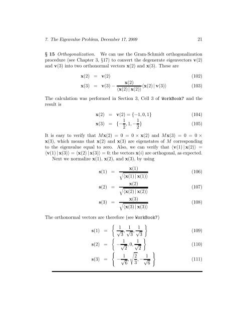
7. The Eigenvalue Problem, December 17, 2009 21 § 15 Orthogonalization. We can use the Gram-Schmidt orthogonalization procedure (see Chapter 3, §17) to convert the degenerate eigenvectors v(2) and v(3) into two orthonormal vectors x(2) and x(3). These are x(2) = v(2) (102) x(3) = x(2) v(3) − x(2) | v(3) x(2) | x(2) (103) The calculation was performed in Section 3, Cell 3 of WorkBook7 and the result is x(2) = v(2) = {−1, 0, 1} (104) x(3) = {− 1 2 , 1, −1 2 } (105) It is easy to verify that Mx(2) = 0 = 0 × x(2) and Mx(3) = 0 = 0 × x(3), which means that x(2) and x(3) are eigenstates of M corresponding to the eigenvalue equal to zero. Also, we can verify that v(1) | x(2) = v(1) | x(3) = x(2) | x(3) =0;thevectorsx(i) are orthogonal, as expected. Next we normalize x(1), x(2), and x(3), by using s(1) = s(2) = s(3) = x(1) x(1) | x(1) (106) x(2) x(2) | x(2) (107) x(3) x(3) | x(3) (108) The orthonormal vectors are therefore (see WorkBook7) s(1) = s(2) = s(3) = 1√3 , 1 1 √ , √ 3 3 − 1 √ 2 , 0, 1 √ 2 ⎧ ⎨ ⎩ − √ 1 ⎫ 2 , 6 3 , − √ 1 ⎬ 6 ⎭ (109) (110) (111)
Page 1 and 2: 7. The Eigenvalue Problem, December
Page 19: 7. The Eigenvalue Problem, December

Chapter 7. The Eigenvalue Problem

You also want an ePaper? Increase the reach of your titles

Delete template?

Save as template?