Jac Romme - Library of Ph.D. Theses | EURASIP
Jac Romme - Library of Ph.D. Theses | EURASIP
Jac Romme - Library of Ph.D. Theses | EURASIP

You also want an ePaper? Increase the reach of your titles
YUMPU automatically turns print PDFs into web optimized ePapers that Google loves.
Channel Fading Statistics and Transmitted-Reference Communication<br />
UWB<br />
<strong>Jac</strong> <strong>Romme</strong><br />
SPSC Dissertation Series
Doctoral Thesis<br />
UWB Channel Fading Statistics and<br />
Transmitted-Reference<br />
Communication<br />
ir. <strong>Jac</strong> <strong>Romme</strong><br />
————————————–<br />
Signal Processing and Speech Communication Laboratory<br />
Graz University <strong>of</strong> Technology, Austria<br />
Supervisor: Univ.-Pr<strong>of</strong>. Dipl.-Ing. Dr.techn. Gernot Kubin<br />
External Evaluator: Pr<strong>of</strong>. Sergio Benedetto<br />
Co-supervisor: Dipl.-Ing. Dr. Klaus Witrisal<br />
Graz, March 2008
“The scientist is not a person who gives the right answers,<br />
he is one who asks the right questions.”<br />
[Claude Lévi-Strauss, 1964]
Zusammenfassung<br />
Die Robustheit der Ultra WideBand (UWB) Übertragung gegenüber Small-Scale-Fading<br />
(SSF) in Mehrwegekanälen als Folge der großen Bandbreite ist hinlänglich bekannt. Dennoch<br />
gibt es bislang kein Modell, das die Variation der Empfangssignalstärke in Abhängigkeit<br />
von der Signalbandbreite und genereller Kanaleigenschaften wie dem Leistungsverzögerungs-Pr<strong>of</strong>il<br />
beschreibt. Ein solches Modell würde dem Kommunikationsingenieur<br />
erlauben, die Nachteile einer großen Bandbreite wie z.B. steigende Systemkomplexität<br />
gegenüber dem Vorteil einer erhöhten Systemrobustheit abwägen zu können. In dieser<br />
Dissertation wird ein Modell vorgestellt, das diese Analyse erstmals ermöglicht, indem es<br />
die statistischen Eigenschaften von SSF als Funktion der Signalbandbreite und des Leistungsverzögerungs-Pr<strong>of</strong>ils<br />
beschreibt. Zudem wird eine Berechnung der resultierenden<br />
Bitfehlerrate bei Verwendung von BPSK Modulation vorgestellt.<br />
Die hohe Bandbreite der UWB-Systeme ist zwar vorteilhaft bei der Bekämpfung von<br />
SSF, führt aber im Empfängerdesign zu Problemen. Kohärente Empfängerkonzepte sind<br />
sehr komplex, so dass bereits in 2002 von den Autoren Tomlinson und Hoctor ein alternatives<br />
Konzept vorgeschlagen wurde, das das Transmitted Reference (TR) Verfahren mit<br />
einem Autokorrelationsempfänger kombiniert und eine Kanalschätzung vermeiden kann.<br />
Aufgrund der nichtlinearen Struktur des Empfängers war es bislang schwierig, sein exaktes<br />
Verhalten vorherzusagen. Diese Dissertation gibt nun Einblicke in das prinzipielle<br />
Verhalten des TR-Autokorrelationsempfängers und zeigt zusätzlich Verbesserungen auf,<br />
die es ermöglichen, einige Nachteile des Konzepts abzuschwächen. Weiterhin werden verschiedene<br />
Interpretationen des TR UWB-Prinzips präsentiert, die z.B. den Einfluss von<br />
Intersymbolinterferenz auf das System erklären.<br />
Basierend auf dem theoretischen Verständnis von TR-UWB wird im Anschluss ein<br />
hochratiges Übertragungssystem mit Datenraten im Bereich von einigen 100 Mbps bei<br />
einer Bandbreite von 1 GHz entwickelt. Es verwendet eine Kombination von trellisbasierter<br />
Entzerrung, Turbo Entzerrung, Turbo-Dekodierung und Verarbeitung in mehreren<br />
Bändern, die es erlaubt, die gewünschte Datenrate mit moderater digitaler Signalverarbeitung<br />
zu erzielen. Bereits ein E b /N 0 von 12 dB ist für eine Bitfehlerrate kleiner<br />
als 10 −6 ausreichend.<br />
i
Abstract<br />
It is well known that Ultra WideBand (UWB) transmission is inherently robust against<br />
small-scale-fading (SSF) that arises in multipath scattering environments, due to its large<br />
signal bandwidth. However, no model with a physical interpretation exists that relates<br />
the variations <strong>of</strong> received signal strength to the signal bandwidth and general channel<br />
parameters, like e.g. the average channel power delay pr<strong>of</strong>ile. Such a model would be <strong>of</strong><br />
relevance for e.g. system designers, who have to make trade<strong>of</strong>fs between system aspects,<br />
like complexity and energy efficiency on one hand, and robustness against small-scalefading<br />
on the other hand. In this thesis, a model is presented that allows for such a trade<strong>of</strong>f<br />
analysis, relating the average power delay pr<strong>of</strong>ile parameters and signal bandwidth to the<br />
statistical properties <strong>of</strong> the SSF. Additionally, it is shown how the uncoded and coded<br />
BER <strong>of</strong> BPSK modulation can be computed in a closed-form for a given average power<br />
delay pr<strong>of</strong>ile and signal bandwidth.<br />
As stated before, UWB communication is inherently resilient against SSF. Unfortunately,<br />
coherent receivers become rather complex in the UWB case. In 2002, Tomlinson<br />
and Hoctor proposed to combine Transmitted Reference (TR) signaling with an autocorrelation<br />
receiver (AcR) for UWB communications, to dispose <strong>of</strong> the need for channel<br />
estimation. Due to the non-linear structure <strong>of</strong> the AcR, little was known with respect to<br />
its behaviour in various situations. This thesis aims to provide better insight in the behaviour<br />
<strong>of</strong> such systems. Not only is the principle <strong>of</strong> TR UWB communication explained,<br />
also several extensions to the TR principle are proposed, which relieve some <strong>of</strong> its drawbacks.<br />
Additionally, novel interpretations for TR UWB systems are presented, which<br />
explain the behaviour <strong>of</strong> TR systems e.g. in the presence <strong>of</strong> inter-symbol-interference.<br />
After understanding the behaviour <strong>of</strong> TR UWB systems, the design <strong>of</strong> a high-rate<br />
TR UWB system is presented that supports data-rates up to 100 Mb/s, while occupying<br />
1 GHz <strong>of</strong> bandwidth. Using a combination <strong>of</strong> trellis-based equalization, multiband processing,<br />
turbo equalization and turbo coding, a system is obtained which is moderately<br />
complex with respect to digital signal processing and requires an E b /N 0 <strong>of</strong> only 12 dB to<br />
obtain a BER better than 10 −6 .<br />
iii
Contents<br />
Zusammenfassung<br />
Abstract<br />
Acronyms<br />
i<br />
iii<br />
ix<br />
1 General Introduction 1<br />
1.1 Wireless Communications . . . . . . . . . . . . . . . . . . . . . . . . . . . 1<br />
1.2 Ultra-WideBand . . . . . . . . . . . . . . . . . . . . . . . . . . . . . . . . 3<br />
1.3 Framework and Objectives . . . . . . . . . . . . . . . . . . . . . . . . . . . 5<br />
1.4 Thesis Outline and Contributions . . . . . . . . . . . . . . . . . . . . . . . 6<br />
2 Theory <strong>of</strong> Fading UWB Channels 13<br />
2.1 Introduction . . . . . . . . . . . . . . . . . . . . . . . . . . . . . . . . . . . 13<br />
2.1.1 The Radio Channel . . . . . . . . . . . . . . . . . . . . . . . . . . . 13<br />
2.1.2 Radio Channel Model . . . . . . . . . . . . . . . . . . . . . . . . . 14<br />
2.1.3 Channel Characterizing Parameters . . . . . . . . . . . . . . . . . . 15<br />
2.1.4 Impact <strong>of</strong> the Channel on Radio Signals . . . . . . . . . . . . . . . 16<br />
2.2 Frequency Domain Properties <strong>of</strong> UWB Channels . . . . . . . . . . . . . . . 18<br />
2.2.1 Frequency Domain Correlation . . . . . . . . . . . . . . . . . . . . 19<br />
2.2.2 Eigenvalues and Their <strong>Ph</strong>ysical Interpretation . . . . . . . . . . . . 20<br />
2.2.3 Asymptotic Behaviour <strong>of</strong> the Eigenvalues . . . . . . . . . . . . . . . 22<br />
2.3 Diversity <strong>of</strong> UWB Channels . . . . . . . . . . . . . . . . . . . . . . . . . . 25<br />
2.3.1 The Mean Power Gain . . . . . . . . . . . . . . . . . . . . . . . . . 26<br />
2.3.2 Statistical Characterization <strong>of</strong> the NLOS Mean Power Gain . . . . . 26<br />
2.3.3 Generalization <strong>of</strong> the Statistics to LOS Scenarios . . . . . . . . . . 28<br />
2.3.4 Diversity Level <strong>of</strong> UWB Channels . . . . . . . . . . . . . . . . . . . 29<br />
2.4 BER on UWB Channels . . . . . . . . . . . . . . . . . . . . . . . . . . . . 31<br />
2.4.1 BER <strong>of</strong> BPSK on Fading Channels . . . . . . . . . . . . . . . . . . 31<br />
2.4.2 Performance Analysis . . . . . . . . . . . . . . . . . . . . . . . . . . 33<br />
2.5 Conclusions . . . . . . . . . . . . . . . . . . . . . . . . . . . . . . . . . . . 35<br />
3 Fading <strong>of</strong> Measured UWB Channels 37<br />
3.1 Introduction . . . . . . . . . . . . . . . . . . . . . . . . . . . . . . . . . . . 37<br />
3.2 Description <strong>of</strong> Radio Channel Measurements . . . . . . . . . . . . . . . . . 37<br />
3.3 Overview <strong>of</strong> Measurement Results . . . . . . . . . . . . . . . . . . . . . . . 38<br />
v
vi<br />
CONTENTS<br />
3.3.1 Delay Domain . . . . . . . . . . . . . . . . . . . . . . . . . . . . . . 38<br />
3.3.2 Frequency Domain . . . . . . . . . . . . . . . . . . . . . . . . . . . 40<br />
3.4 Principal Components <strong>of</strong> Measured UWB Channels . . . . . . . . . . . . . 43<br />
3.4.1 Estimation <strong>of</strong> the Eigenvalues and Principal Components . . . . . . 43<br />
3.4.2 Verification <strong>of</strong> the NLOS Eigenvalues and Principal Components . . 44<br />
3.4.3 Verification <strong>of</strong> the LOS Eigenvalues and Principal Components . . . 46<br />
3.5 Analysis <strong>of</strong> the Mean Power Gain . . . . . . . . . . . . . . . . . . . . . . . 46<br />
3.5.1 Estimation <strong>of</strong> the Diversity Level . . . . . . . . . . . . . . . . . . . 47<br />
3.5.2 Verification <strong>of</strong> the Diversity Level . . . . . . . . . . . . . . . . . . . 48<br />
3.5.3 Verification <strong>of</strong> the Mean Power Gain . . . . . . . . . . . . . . . . . 49<br />
3.6 BER Comparison on Measured and Theoretical UWB Channels . . . . . . 51<br />
3.7 Conclusions . . . . . . . . . . . . . . . . . . . . . . . . . . . . . . . . . . . 53<br />
4 Theory <strong>of</strong> TR UWB Communications 57<br />
4.1 Introduction . . . . . . . . . . . . . . . . . . . . . . . . . . . . . . . . . . . 57<br />
4.2 Principle <strong>of</strong> Transmitted Reference Communication . . . . . . . . . . . . . 58<br />
4.2.1 Transmitted-Reference Signaling . . . . . . . . . . . . . . . . . . . . 58<br />
4.2.2 Autocorrelation Receiver . . . . . . . . . . . . . . . . . . . . . . . . 58<br />
4.2.3 The Drawbacks . . . . . . . . . . . . . . . . . . . . . . . . . . . . . 61<br />
4.2.4 Implementation Considerations . . . . . . . . . . . . . . . . . . . . 61<br />
4.3 Extensions <strong>of</strong> the TR Principle . . . . . . . . . . . . . . . . . . . . . . . . 62<br />
4.3.1 Weighted Autocorrelation and Fractional Sampling AcR . . . . . . 62<br />
4.3.2 Complex-Valued Autocorrelation Receiver . . . . . . . . . . . . . . 65<br />
4.3.3 TR M-ary <strong>Ph</strong>ase Shift Keying . . . . . . . . . . . . . . . . . . . . . 67<br />
4.4 Generic TR System Model . . . . . . . . . . . . . . . . . . . . . . . . . . . 68<br />
4.4.1 Introduction . . . . . . . . . . . . . . . . . . . . . . . . . . . . . . . 68<br />
4.4.2 Continuous-Time System Model . . . . . . . . . . . . . . . . . . . . 68<br />
4.4.3 Discrete-Time Equivalent System Model . . . . . . . . . . . . . . . 69<br />
4.5 Interpretation <strong>of</strong> the TR System Model . . . . . . . . . . . . . . . . . . . . 72<br />
4.5.1 Introduction . . . . . . . . . . . . . . . . . . . . . . . . . . . . . . . 72<br />
4.5.2 Vector Notation for Volterra Kernels . . . . . . . . . . . . . . . . . 75<br />
4.5.3 Extension <strong>of</strong> the Vector Notation . . . . . . . . . . . . . . . . . . . 77<br />
4.5.4 Linear MIMO Model . . . . . . . . . . . . . . . . . . . . . . . . . . 78<br />
4.5.5 Data Model as Finite State Machine . . . . . . . . . . . . . . . . . 79<br />
4.5.6 Reduced Memory Data Model . . . . . . . . . . . . . . . . . . . . . 82<br />
4.6 Statistical Properties <strong>of</strong> the TR System Model . . . . . . . . . . . . . . . . 84<br />
4.6.1 Statistics <strong>of</strong> the Signal Term . . . . . . . . . . . . . . . . . . . . . . 85<br />
4.6.2 Statistics <strong>of</strong> the Gaussian Noise Term . . . . . . . . . . . . . . . . . 85<br />
4.6.3 Statistics <strong>of</strong> the Non-Gaussian Noise Term . . . . . . . . . . . . . . 87<br />
4.6.4 Analysis <strong>of</strong> the Noise Term . . . . . . . . . . . . . . . . . . . . . . . 88<br />
4.7 Conclusions . . . . . . . . . . . . . . . . . . . . . . . . . . . . . . . . . . . 90<br />
5 Analysis <strong>of</strong> TR UWB Communication 91<br />
5.1 Introduction . . . . . . . . . . . . . . . . . . . . . . . . . . . . . . . . . . . 91<br />
5.2 Description <strong>of</strong> the Linear Weighting . . . . . . . . . . . . . . . . . . . . . . 91<br />
5.3 System Performance in the Absence <strong>of</strong> ISI . . . . . . . . . . . . . . . . . . 92
CONTENTS<br />
vii<br />
5.3.1 Influence <strong>of</strong> the Weighting Criteria and Fractional Sampling Rate . 93<br />
5.3.2 Influence <strong>of</strong> Delay and Fractional Sampling Rate . . . . . . . . . . . 94<br />
5.3.3 Influence <strong>of</strong> Bandwidth . . . . . . . . . . . . . . . . . . . . . . . . . 95<br />
5.3.4 Influence <strong>of</strong> Modulation . . . . . . . . . . . . . . . . . . . . . . . . 95<br />
5.4 System Performance in the Presence <strong>of</strong> ISI . . . . . . . . . . . . . . . . . . 97<br />
5.4.1 Influence <strong>of</strong> the Weighting Criteria and Fractional Sampling Rate . 97<br />
5.4.2 Influence <strong>of</strong> Bandwidth . . . . . . . . . . . . . . . . . . . . . . . . . 98<br />
5.4.3 Influence <strong>of</strong> Modulation . . . . . . . . . . . . . . . . . . . . . . . . 98<br />
5.5 Conclusions . . . . . . . . . . . . . . . . . . . . . . . . . . . . . . . . . . . 100<br />
6 Design <strong>of</strong> a High-Rate TR UWB System 103<br />
6.1 Introduction . . . . . . . . . . . . . . . . . . . . . . . . . . . . . . . . . . . 103<br />
6.2 Design Considerations for a High-Rate TR UWB System . . . . . . . . . . 103<br />
6.2.1 Trellis-Based Equalization . . . . . . . . . . . . . . . . . . . . . . . 103<br />
6.2.2 Power Spectral Density <strong>of</strong> TR Signals . . . . . . . . . . . . . . . . . 104<br />
6.2.3 Volterra System Identification . . . . . . . . . . . . . . . . . . . . . 105<br />
6.2.4 Multiband Transmitted Reference . . . . . . . . . . . . . . . . . . . 106<br />
6.2.5 The Role <strong>of</strong> Forward Error Control . . . . . . . . . . . . . . . . . . 106<br />
6.2.6 Principle <strong>of</strong> Turbo Equalization . . . . . . . . . . . . . . . . . . . . 107<br />
6.3 System Description . . . . . . . . . . . . . . . . . . . . . . . . . . . . . . . 108<br />
6.3.1 Description <strong>of</strong> the TX Architecture and RX RF Front-End . . . . . 108<br />
6.3.2 Forward Error Control . . . . . . . . . . . . . . . . . . . . . . . . . 109<br />
6.3.3 Turbo Equalization . . . . . . . . . . . . . . . . . . . . . . . . . . . 110<br />
6.3.4 SISO Decoder Structure . . . . . . . . . . . . . . . . . . . . . . . . 112<br />
6.3.5 Stop Algorithm . . . . . . . . . . . . . . . . . . . . . . . . . . . . . 114<br />
6.3.6 Measure <strong>of</strong> Complexity . . . . . . . . . . . . . . . . . . . . . . . . . 114<br />
6.4 Performance Analysis . . . . . . . . . . . . . . . . . . . . . . . . . . . . . . 115<br />
6.4.1 Impact <strong>of</strong> Equalizer Complexity Without Turbo Equalization . . . . 115<br />
6.4.2 Benefit <strong>of</strong> Turbo Equalization . . . . . . . . . . . . . . . . . . . . . 117<br />
6.5 Conclusions . . . . . . . . . . . . . . . . . . . . . . . . . . . . . . . . . . . 119<br />
7 Conclusions and Recommendations 123<br />
A Estimation <strong>of</strong> the Nakagami-m Parameter 127<br />
B Complex-Valued AcR 135<br />
C PSD <strong>of</strong> Scrambled QPSK-TR UWB Signals 137<br />
D Derivation <strong>of</strong> the Log-MAP Algorithm 139<br />
Bibliography 143<br />
Acknowledgments 153<br />
Curriculum Vitae 155
viii<br />
CONTENTS
Acronyms<br />
1G<br />
2G<br />
3G<br />
4G<br />
ADC<br />
AcR<br />
AMPS<br />
APDP<br />
AWGN<br />
BCJR<br />
BER<br />
BPF<br />
BPSK<br />
CC<br />
CDF<br />
CEPT<br />
CEV<br />
CFR<br />
CIR<br />
CV<br />
CW<br />
First Generation<br />
Second Generation<br />
Third Generation<br />
Fourth Generation<br />
Analogue to Digital Converter<br />
Autocorrelation Receiver<br />
American Advanced Mobile <strong>Ph</strong>one System<br />
Average Power Delay Pr<strong>of</strong>ile<br />
Additive White Gaussian Noise<br />
Bahl, Cocke, Jelinek and Raviv<br />
Bit Error Rate<br />
Band Pass Filter<br />
Binary-<strong>Ph</strong>ase-Shift-Keying<br />
Convolutional Code<br />
Cumulative Distribution Function<br />
European Conference <strong>of</strong> Postal and Telecommunications<br />
Administrations<br />
Circulant Eigenvalue<br />
Channel Frequency Response<br />
Channel Impulse Response<br />
Complex-Valued<br />
Carrier Wave<br />
ix
x<br />
CONTENTS<br />
DAA<br />
DARPA<br />
DFT<br />
DLL<br />
DS<br />
DSL<br />
DSP<br />
DS-UWB<br />
ECC<br />
ECMA<br />
EM<br />
FCC<br />
FDM<br />
FEC<br />
FER<br />
FH<br />
FIR<br />
HMM<br />
FSFC<br />
FSM<br />
FSR<br />
I&D<br />
IEEE<br />
ISI<br />
ISP<br />
ITU-R<br />
LLV<br />
Detect and Avoid<br />
Defence Advanced Research Projects Agency<br />
Discrete Fourier Transform<br />
Data Link Layer<br />
Direct Sequence<br />
Digital Subscriber Loop<br />
Digital Signal Processing<br />
Direct Sequence - UWB<br />
Electronic Communications Committee<br />
European Computer Manufacturers Association<br />
Electro-Magnetic<br />
Federal Communications Commission<br />
Full Data Model<br />
Forward Error Control<br />
Frame Error Rate<br />
Frequency Hopping<br />
Finite Impulse Response<br />
Hidden Markov Model<br />
Frequency Selective Fading Channel<br />
Finite State Machine<br />
Fractional Sampling Rate<br />
Integrate and Dump<br />
Institute <strong>of</strong> Electrical and Electronics Engineers<br />
Inter Symbol Interference<br />
Internet Service Provider<br />
International Telecommunication Union Radiocommunication Sector<br />
Log-Likelihood Value
CONTENTS<br />
xi<br />
LMS<br />
LOS<br />
LPF<br />
LS<br />
MAC<br />
MAP<br />
MB-OFDM<br />
MIC<br />
MIMO<br />
MLSD<br />
MMSE<br />
MPG<br />
MRC<br />
NLOS<br />
NMT<br />
OFDM<br />
OSI<br />
PC<br />
PCA<br />
PDF<br />
PDP<br />
PHY<br />
PIAM<br />
PN<br />
PPM<br />
PSD<br />
QAM<br />
Least Mean Square<br />
Line-<strong>of</strong>-Sight<br />
Low Pass Filter<br />
Least Squares<br />
Multiple Access Layer <strong>of</strong> the OSI model<br />
Maximum A-Posteriori<br />
Multi-Band Orthogonal Frequency Division Multiplexing<br />
Ministry <strong>of</strong> Internal Affairs and Communications<br />
Multiple-Input, Multiple-Output<br />
Maximum-Likelihood Sequence Detection<br />
Minimum Mean Square Error<br />
Mean Power Gain<br />
Maximum Ratio Combining<br />
Non-Line-<strong>of</strong>-Sight<br />
Scandinavian Nordic Mobile Telephone<br />
Orthogonal Frequency Division Multiplexing<br />
Open Systems Interconnection<br />
Principal Component<br />
Principal Component Analysis<br />
Probability Density Function<br />
Power Delay Pr<strong>of</strong>ile<br />
<strong>Ph</strong>ysical Layer <strong>of</strong> the OSI model<br />
Pulse Interval and Amplitude Modulation<br />
Pseudo Noise<br />
Pulse Position Modulation<br />
Power Spectral Density<br />
Quadrature Amplitude Modulation
xii<br />
CONTENTS<br />
QPSK<br />
R&O<br />
RF<br />
RMDM<br />
RMS<br />
RSCC<br />
RV<br />
RX<br />
SIMO<br />
SISO<br />
SNIR<br />
SNR<br />
SOVA<br />
SSF<br />
SVD<br />
TACS<br />
TG3a<br />
TR<br />
TX<br />
UB<br />
US<br />
USB<br />
UWB<br />
VOIP<br />
WPAN<br />
WLAN<br />
WMAN<br />
WWAN<br />
WRAN<br />
Quadrature-<strong>Ph</strong>ase-shift-Keying<br />
Report and Order<br />
Radio Frequency<br />
Reduced Memory Data Model<br />
Root Mean Square<br />
Recursive Systematic Convolutional Code<br />
Random Value<br />
Receiver<br />
Single-Input, Multiple-Output<br />
S<strong>of</strong>t-Input, S<strong>of</strong>t-Output<br />
Signal-to-Noise-and-Interference Ratio<br />
Signal-to-Noise Ratio<br />
S<strong>of</strong>t-Output Viterbi Algorithm<br />
Small-Scale Fading<br />
Singular Value Decomposition<br />
British Total Access Communication System<br />
Task Group 3a<br />
Transmitted Reference<br />
Transmitter<br />
Upper Bound<br />
Uncorrelated Scattering<br />
Universal Serial Bus<br />
Ultra-Wideband<br />
Voice over IP<br />
Wireless Personal Area Network<br />
Wireless Local Area Network<br />
Wireless Metropolitan Area Network<br />
Wireless Wide Area Network<br />
Wireless Regional Area Network
Chapter 1<br />
General Introduction<br />
1.1 Wireless Communications<br />
In the 1860s, James Clerk Maxwell, a Scottish physicist, proposed a set <strong>of</strong> differential<br />
equations, which together describe the behaviour <strong>of</strong> electric and magnetic fields, as well<br />
as their interactions with each other and matter. Based on these equations, he predicted<br />
the existence <strong>of</strong> self-sustaining, oscillating waves composed out <strong>of</strong> an electric and magnetic<br />
field that travel through space. Nowadays, these waves are referred to as electro-magnetic<br />
waves. Also he was the first to propose that light is a type <strong>of</strong> electromagnetic wave.<br />
Through experimentation using a spark-gap transmitter and a spark-gap loop antenna<br />
as detector, Heinrich Rudolph Hertz proved in 1886 that a spark at the transmitter can<br />
induce a spark at the receiver, showing that electromagnetic waves can travel through<br />
free space over some distance, as Maxwell predicted.<br />
Fascinated by these results, Lodge, Marconi and Popov began almost simultaneously<br />
transforming radio into a way <strong>of</strong> wireless communication. In 1896, Marconi and Popov<br />
both sent radio messages over short distances. In 1899, Marconi signalled the first wireless<br />
signal across the English Channel and two years later, he already telegraphed from<br />
England to Newfoundland. These experiments made the world considerably smaller, since<br />
now the transport <strong>of</strong> information was only limited by the speed <strong>of</strong> light.<br />
Nowadays, the use <strong>of</strong> wireless communications for the transport <strong>of</strong> voice and data<br />
has been integrated into everyday’s life. The penetration <strong>of</strong> mobile telephony in the<br />
western world is <strong>of</strong>ten above 80% and the deployment <strong>of</strong> wireless local area networks has<br />
become normal. It is therefore hard to imagine that only as recently as the early nineties,<br />
commercial wireless communications was a rare commodity for many.<br />
After the introduction <strong>of</strong> First Generation (1G) mobile radio telephony, the success<br />
<strong>of</strong> wireless communications started. The 1G mobile radio telephony emerged in the<br />
early eighties, although in its early years the term portable communications was more<br />
appropriate. Due to limitations in technology, these phones deployed analogue modulation<br />
and were still rather big. These systems were developed for voice communication only and<br />
every country used their own frequency bands, disabling the possibility <strong>of</strong> international<br />
roaming. Nevertheless, these systems allowed for the opening <strong>of</strong> a mass-market for wireless<br />
voice communication. Some <strong>of</strong> the most successful 1G systems were American Advanced<br />
Mobile <strong>Ph</strong>one System (AMPS), British Total Access Communication System (TACS) and<br />
1
2 CHAPTER 1. GENERAL INTRODUCTION<br />
Scandinavian Nordic Mobile Telephone (NMT).<br />
With the introduction <strong>of</strong> Second Generation (2G) systems, a true revolution took<br />
place in the use <strong>of</strong> mobile radio telephony. The reasons for their success are manifold.<br />
Not only used 2G digital modulation, but more importantly 2G was standardized. As<br />
a result, devices became significantly smaller, cheaper, allowed for international roaming<br />
and had longer operating time on single charge <strong>of</strong> battery. All these aspects contributed<br />
to the success <strong>of</strong> 2G.<br />
The commercial success <strong>of</strong> 2G together with the Internet boom, caused an explosion <strong>of</strong><br />
developments to penetrate mobile communications further into everyday’s life. Nowadays,<br />
many wireless communication systems are in use aside each other, each developed for its<br />
own application scenarios.<br />
Roughly speaking, five network types can be distinguished, namely WPAN, WLAN,<br />
WMAN, WWAN and WRAN. No strict definitions exist to distinguish between them and<br />
<strong>of</strong>ten the terms are used more for market-technical reasons than technical ones. Standards<br />
belonging to different types may therefore compete with each other for the grace <strong>of</strong> the<br />
customers. Nevertheless, we will make an effort to characterize them coarsely:<br />
A Wireless Personal Area Network (WPAN) is a network technology to interconnect<br />
devices around a workspace or person using wireless radio technology. The typical range<br />
is around 10 meters and <strong>of</strong>ten mobility is not supported, meaning that the connection<br />
breaks down when leaving the coverage area.<br />
A Wireless Local Area Network (WLAN) is used to connect computers and other<br />
WLAN enabled devices to the wired network directly via base-stations. The range covered<br />
by a base-station is on the order <strong>of</strong> 100 m depending on the environment. Furthermore,<br />
a network <strong>of</strong> base-stations can be installed to support mobility within the area covered<br />
by the network <strong>of</strong> base-stations.<br />
Wireless Metropolitan Area Network (WMAN) is basically an extension <strong>of</strong> the WLAN<br />
concept to support ranges in the order <strong>of</strong> 1 km, such that with less base-stations a larger<br />
area can be covered reducing the cost <strong>of</strong> the infra-structure. An Internet Service Provider<br />
(ISP) managing the WMAN network will provide Internet access to its subscribers as an<br />
alternative for cable and Digital Subscriber Loop (DSL). Most likely, access the Internet<br />
is limited to the coverage area <strong>of</strong> the ISP and the underlying technology supports only<br />
moderate velocities. Nevertheless, WMAN could go in competition with the cellular<br />
network operators, especially now Voice over IP (VOIP) is taking <strong>of</strong>f as well.<br />
The term Wireless Wide Area Network (WWAN) is typically used for standards developed<br />
by/for the cellular network operators. The typical range is 10 km and differs from<br />
WLAN and WMAN, because <strong>of</strong> the use <strong>of</strong> cellular network technology. These cellular<br />
technologies provide for nationwide and international access using roaming. In this sense<br />
WWAN provides higher mobility and higher velocities.<br />
A recent development is the Wireless Regional Area Network (WRAN) introduced by<br />
Institute <strong>of</strong> Electrical and Electronics Engineers (IEEE) standard 802.22, which has as<br />
mandate to develop a standard for a cognitive radio-based PHY/MAC/air interface for<br />
use by license-exempt devices in spectrum allocated to TV Broadcasting. The target application<br />
<strong>of</strong> WRANs is wireless broadband Internet access in areas with sparse costumers,<br />
such as rural areas and developing countries. As a result, the typical coverage range <strong>of</strong> a<br />
single base station is aimed to be up to 100 km to reduce the cost <strong>of</strong> the infra-structure.
1.2. ULTRA-WIDEBAND 3<br />
∼ 100 km<br />
WRAN<br />
802.22<br />
Standard<br />
∼ 10 km<br />
Under development<br />
max range<br />
WWAN<br />
∼ 1 km<br />
WMAN<br />
∼ 100 m<br />
GSM<br />
GPRS<br />
EDGE<br />
UMTS<br />
802.20<br />
HSDPA<br />
WiMax<br />
3G-LTE<br />
802.16d/e<br />
UWB Standard<br />
WLAN<br />
∼ 10 m<br />
802.11 11b 11a/g<br />
11n<br />
WPAN<br />
ZigBee Bleutooth 802.15.4a WiMedia 802.15.3c<br />
(W-USB)<br />
TerraHz<br />
10 kb/s 100 kb/s 1 Mb/s 10 Mb/s 100 Mb/s 1 Gb/s 10 Gb/s<br />
data rate<br />
100 Gb/s<br />
Figure 1.1: Overview <strong>of</strong> communication standards<br />
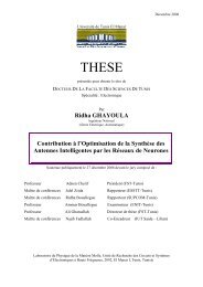
Another way to distinguish standards is with respect to supported data rates. Typically,<br />
recent standards provide higher data rates than the older ones. When violating this<br />
general rule, the new standard will have some distinct benefits with respect to existing<br />
ones, e.g., with respect to cost or added functionality like ranging or localization. An<br />
overview <strong>of</strong> currently successful standards and promising future standards can be found<br />
in Fig. 1.1, separated with respect to coverage area and data rate. The overview contains<br />
two standards related to the topic <strong>of</strong> this thesis, namely 802.15.4a and WiMedia. These<br />
will be discussed in more detail in Sec. 1.2. More details on the other radio communication<br />
standards can be found in [1, 2, 3].<br />
1.2 Ultra-WideBand<br />
Although Ultra-Wideband (UWB) is <strong>of</strong>ten considered a new radio technology, UWB<br />
technology has been around for many years. In fact, the first wireless transmission experiments<br />
conducted by Hertz and Marconi could be considered a pulse based UWB.<br />
The use <strong>of</strong> a spark gap to generate radio signals inherently results in the radiation <strong>of</strong><br />
a pulse that is UWB. Radio communications took another course with the invention<br />
<strong>of</strong> the Alexanderson radio alternator radio-frequency source, which allowed for Carrier<br />
Wave (CW) communications. Not only because CW allowed for simpler transmitters, but<br />
also because the low bandwidth <strong>of</strong> CW signals allowed selective Band Pass Filters (BPFs)<br />
to be used in the receiver to block out most <strong>of</strong> the noise and interference. Therefore, radio<br />
regulatory bodies started to assign frequency bands to specific systems, such that they<br />
could co-exist without interfering with each other.<br />
The success <strong>of</strong> CW systems resulted in UWB to be forgotten for more than 60 years.<br />
The interest in UWB came back with the invention <strong>of</strong> sub-nanosecond pulse generators in
4 CHAPTER 1. GENERAL INTRODUCTION<br />
the sixties. Shortly after, the potential <strong>of</strong> UWB for radio communications was identified,<br />
eventually resulting in the first US patent on pulse-based UWB radio communications<br />
in 1973 [4]. In those days, the main applications were radar and positioning, because<br />
<strong>of</strong> the inherent ability <strong>of</strong> UWB to resolve objects with a high spatial resolution, and<br />
military communication systems, because <strong>of</strong> the inherent covertness <strong>of</strong> UWB signals.<br />
Most developments were therefore conducted in the military or funded by governments<br />
under classified programs. Interestingly, UWB in those days was called either baseband,<br />
carrier-free or impulse technology. The term UWB itself was first used in a radar study<br />
by the Defence Advanced Research Projects Agency (DARPA) in 1990. Despite these<br />
early developments, CW remained to govern commercial wireless radio communications.<br />
The interest in UWB for commercial wireless radio communications revived with a<br />
series <strong>of</strong> papers by Scholtz and Win [5, 6, 7] and the UWB activities <strong>of</strong> U.S. based companies<br />
like XtremeSpectrum, Multispectral Solutions and Time Domain. The lobbying<br />
activities <strong>of</strong> these companies resulted in a Notice <strong>of</strong> Inquiry by the Federal Communications<br />
Commission (FCC) in September 1998 on the allowance <strong>of</strong> UWB on an unlicensed<br />
basis under Part 15 <strong>of</strong> its rules [8]. This eventually led to a Report and Order (R&O)<br />
<strong>of</strong> the FCC in February 2002, to allow UWB under part 15 <strong>of</strong> its regulation [9]. Here,<br />
UWB emitters are allowed to operate in a frequency band from 3.1 to 10.6 GHz with a<br />
Power Spectral Density (PSD) <strong>of</strong> -41.3 dBm/MHz, the same as allowed by part 15 for<br />
unintentional radiators. The main intent <strong>of</strong> the R&O is to provide re-use <strong>of</strong> scarce radio<br />
spectrum while enabling high data rate WPAN as well as radar, imaging and localization<br />
systems.<br />
At first, UWB was thought to be a pulse-based system, but the FCC defined UWB in<br />
terms <strong>of</strong> a transmission from an antenna for which the emitted signal bandwidth exceeds<br />
the lesser <strong>of</strong> 500 MHz or 20% <strong>of</strong> the center frequency. This allows Orthogonal Frequency<br />
Division Multiplexing (OFDM) and Direct Sequence (DS) systems to be operated under<br />
the UWB regulation. The opening <strong>of</strong> several GHz <strong>of</strong> bandwidth for commercial applications<br />
resulted in an avalanche <strong>of</strong> academic research and industrial efforts, which eventually<br />
lead to the standardization <strong>of</strong> UWB for WPAN [10, 11].<br />
The road to standardization has been rather rocky. In December 2002, the IEEE<br />
granted the project authorization request as Task Group 3a (TG3a) part <strong>of</strong> the 802.15<br />
standards family for WPAN. The aim <strong>of</strong> TG3a was to specify a standard PHY for<br />
high-data-rate, short-range, low-power, and low-cost wireless networking technology using<br />
UWB. In total 23 UWB PHY specifications were submitted, which quickly merged into<br />
two proposals. The WiMedia Alliance proposed a Multi-Band Orthogonal Frequency<br />
Division Multiplexing (MB-OFDM) PHY, which is a combination <strong>of</strong> Frequency Hopping<br />
(FH) and OFDM, while the UWB Forum proposed a Direct Sequence - UWB (DS-UWB)<br />
PHY. Over two and a half years, both consortia debated to come to a single PHY-proposal.<br />
Eventually, both agreed to not agree, resulting in a withdrawal <strong>of</strong> TG3a.<br />
The withdrawal <strong>of</strong> TG3a did not mean the end <strong>of</strong> UWB for high-data-rate WPAN.<br />
Both parties continued their effort on their own. In December 2005, the European Computer<br />
Manufacturers Association (ECMA) released two ISO-based standards for UWB<br />
based on the WiMedia UWB proposal [10, 11]. It supports data rates up to 480 Mb/s,<br />
but future extensions are expected to support data rates above 1 Gb/s. Furthermore, the<br />
WiMedia PHY has been selected for wireless Universal Serial Bus (USB) under the name
1.3. FRAMEWORK AND OBJECTIVES 5<br />
Certified Wireless USB [12]. After initial activities <strong>of</strong> the UWB Forum, it became rather<br />
quiet after the Freescale’s departure from the UWB Forum. Therefore, it seems that the<br />
WiMedia Alliance is winning the race.<br />
Besides UWB being considered for high data rate WPAN, also joint low data rate<br />
and localization is considered for WPAN. In March 2004, the IEEE launched task group<br />
802.15.4a for a mandate to develop an alternative PHY as optional extension to the<br />
802.15.4 PHY, which provides low data rate communications and high precision ranging/location<br />
capability, while being low power and low cost. In March 2007, P802.15.4a<br />
was approved as a new amendment to 802.15.4 by the IEEE. Besides the mandatory<br />
DSSS PHY <strong>of</strong> 802.15.4, one <strong>of</strong> the two alternative PHYs in 802.15.4a provides UWB in<br />
three frequency bands, allowing for data rates between 110 kb/s up to 27.24 Mb/s and<br />
localization [13].<br />
Following the FCC, the International Telecommunication Union Radiocommunication<br />
Sector (ITU-R) has published a Report and Recommendation on UWB in November<br />
<strong>of</strong> 2005. National bodies are expected to adopt their regulation to allow UWB. In<br />
September 2005, a draft decision was released by the European Conference <strong>of</strong> Postal and<br />
Telecommunications Administrations (CEPT). In March 2006, the Electronic Communications<br />
Committee (ECC) decision was issued, allowing UWB for frequencies between<br />
6 and 8.5 GHz. The frequencies between 3.1 and 4.8 GHz are expected to follow soon.<br />
In Japan, the Ministry <strong>of</strong> Internal Affairs and Communications (MIC) launched a regulatory<br />
proposal. The foreseen allocated bandwidths are the frequencies between 3.4 until<br />
4.8 GHz and 7.25 until 10.25 GHz, with the same PSD limits as allowed by the FCC. In<br />
contrast to the FCC, the European and Japanese regulation bodies may demand UWB<br />
systems to use so-called Detect and Avoid (DAA) to avoid interference with current and<br />
future wireless services [14, 15].<br />
1.3 Framework and Objectives<br />
The work presented in this thesis is the partial outcome <strong>of</strong> an objective defined at the<br />
IMST GmbH to develop understanding on UWB technology. Starting in 2000, the objective<br />
was to acquire know-how on the theory and implementation <strong>of</strong> low-cost UWB<br />
systems for communication and localization. The objective resulted in the participation<br />
in several projects both on a European level as well as on a regional level. The projects<br />
funded by the 5-th and 6-th framework <strong>of</strong> the IST program <strong>of</strong> the European Union in a<br />
chronological order are Whyless.com, Europcom and Pulsers 2. The projects funded in<br />
the scope <strong>of</strong> the Nordrhein-Westfalen Zukunftswettbewerb are Bison and PulsOn<br />
While having many benefits, the implementation <strong>of</strong> UWB systems is significantly more<br />
complex than those <strong>of</strong> narrowband systems, since many <strong>of</strong> the hardware components must<br />
be well-behaving over a larger frequency range. Crudely spoken, more bandwidth more<br />
problems, at least with respect to implementation and cost. On the other hand, one<br />
would like to take advantage <strong>of</strong> the fundamental benefits <strong>of</strong> UWB. Hence, during system<br />
design a trade-<strong>of</strong>f is required between both aspects. One <strong>of</strong> the benefits <strong>of</strong> UWB<br />
is inherent resilience against small-scale-fading, which allows the <strong>Ph</strong>ysical Layer <strong>of</strong> the<br />
OSI model (PHY) to operate with higher energy efficiency. The first aim <strong>of</strong> this thesis<br />
is to understand and mathematically model the Small-Scale Fading (SSF) behaviour <strong>of</strong>
6 CHAPTER 1. GENERAL INTRODUCTION<br />
Chapter 1:<br />
General Introduction<br />
Chapter 2:<br />
Theory <strong>of</strong> fading UWB channels<br />
Chapter 4:<br />
Theory <strong>of</strong> TR UWB communication<br />
Chapter 3:<br />
Fading <strong>of</strong> measured UWB channels<br />
Chapter 5:<br />
Analysis <strong>of</strong> TR UWB communication<br />
Chapter 6:<br />
Design <strong>of</strong> a high-rate TR UWB system<br />
Figure 1.2: Organization <strong>of</strong> the thesis<br />
the UWB radio channel to ultimately allow for an educated trade-<strong>of</strong>f between system<br />
performance and complexity. Having low-cost and low-complexity in mind, the second<br />
aim <strong>of</strong> the work is to model and understand the fundamental behaviour <strong>of</strong> UWB wireless<br />
communications using Transmitted Reference (TR) signaling and Autocorrelation<br />
Receivers (AcRs). Based on the developed understanding on UWB, SSF and UWB TR<br />
communications, the final aim is to design a low-cost UWB PHY for WPAN operating<br />
at a data rate <strong>of</strong> 100 Mb/s to unveil the potential <strong>of</strong> UWB TR communications.<br />
1.4 Thesis Outline and Contributions<br />
In this section, the outline and the scientific contributions <strong>of</strong> the thesis are presented.<br />
After the general introduction to the topic presented in this chapter, the thesis outline<br />
follows two parallel branches, which can be read and understood independently. The first<br />
branch consists <strong>of</strong> the subsequent Chapters 2 and 3, which deal with the theory and<br />
practice <strong>of</strong> SSF on UWB channels, respectively. The second branch deals with the theory<br />
and practice <strong>of</strong> TR UWB systems in Chapter 4 and 5, respectively. The insight gained<br />
in both branches is used for the design <strong>of</strong> a high-rate TR-UWB system in Chapter 6. A<br />
graphical impression <strong>of</strong> the thesis outline can be found in Fig. 1.2.<br />
In the following, a short summary <strong>of</strong> each chapter is presented, including the author’s<br />
contributions.<br />
Chapter 2<br />
Chapter 2 relates the statistics <strong>of</strong> SSF on UWB channels and its dependence on bandwidth<br />
in closed-form. By assuming Uncorrelated Scattering (US), first a statistical model is
1.4. THESIS OUTLINE AND CONTRIBUTIONS 7<br />
presented for radio channels in the frequency domain. Based on US, the eigenvalues<br />
are derived in closed-form for UWB channels. Using the eigenvalues, the expectation,<br />
variance and diversity level is derived in closed form both for Line-<strong>of</strong>-Sight (LOS) and<br />
Non-Line-<strong>of</strong>-Sight (NLOS) UWB channels. The diversity level is shown to scale linearly<br />
with respect to the Root Mean Square (RMS)-delay-spread-by-bandwidth product, both<br />
for LOS and NLOS channels.<br />
Finally, upper bounds for the uncoded and coded Bit Error Rate (BER) for ideal UWB<br />
systems will be presented using the eigenvalues <strong>of</strong> the channel. These bounds allow for a<br />
trade-<strong>of</strong>f analysis between bandwidth and BER performance <strong>of</strong> UWB systems on NLOS<br />
UWB channels. Assuming a typical RMS delay spread for indoor environments, the<br />
upper bound for the performance <strong>of</strong> Multiband OFDM systems using frequency hopping<br />
is found to be only 1 dB less energy efficient than an infinite bandwidth system.<br />
The main contributions are:<br />
• Introduction <strong>of</strong> a single measure to quantify the diversity level <strong>of</strong> (UWB) radio<br />
channels [16].<br />
• Derivation <strong>of</strong> a lower bound for the diversity level <strong>of</strong> UWB channels, which converges<br />
to the actual diversity level with increasing bandwidth. The lower bound shows a<br />
linear relationship between the diversity level, bandwidth and RMS-delay-spread,<br />
both for LOS and NLOS channels. This relationship is well-known, but, to our<br />
knowledge, has never derived before in closed form. [to be published].<br />
Chapter 3<br />
In Chapter 3, the theoretical model presented in Chapter 2 is verified using measurement<br />
data <strong>of</strong> UWB radio channels both emphasizing its strengths and short-comings. Firstly,<br />
the channel measurement campaign is described briefly. The statistical properties <strong>of</strong> the<br />
model are validated using the measurement data in both the time and frequency domain.<br />
The statistical properties <strong>of</strong> the Principal Components (PCs) <strong>of</strong> the measured UWB radio<br />
channel have been analyzed. The diversity level as function <strong>of</strong> bandwidth <strong>of</strong> measured<br />
radio channels is compared with the theoretical results. Finally, the BER predicted by<br />
theory is compared with the BER on measured channels.<br />
The main contributions are:<br />
• On NLOS channels, the theoretical model was found to be reasonably accurate, but<br />
not exact because the independence assumption <strong>of</strong> the PC is not valid for the used<br />
measurement data. It is expected that a better prediction is obtained for richer<br />
multipath environments. [to be published].<br />
• For LOS channels, the predicted diversity level <strong>of</strong> the theoretical model is considerably<br />
lower than for measured LOS channels. In practice, the LOS eigenvalue does<br />
not share a PC-dimension with the largest NLOS eigenvalue, but one which is considerably<br />
smaller. The result is considerably less fading. The mechanism(s) behind<br />
have not been unveiled. [to be published].
8 CHAPTER 1. GENERAL INTRODUCTION<br />
Chapter 4<br />
Firstly, a brief introduction <strong>of</strong> TR signaling is presented including its strengths and shortcomings<br />
with respect to performance and implementation. To overcome some <strong>of</strong> these<br />
shortcomings, several extensions <strong>of</strong> the TR principle are proposed. First, a fractional<br />
sampling AcR structure is proposed to relax synchronization and allow for weighted<br />
autocorrelation, while simplifying the implementation. Second, a complex-valued AcR<br />
is proposed to make the system less sensitive against delay mismatches. Additionally,<br />
complex-valued modulation for TR signaling is proposed. To understand the system’s<br />
behaviour, a general-purpose discrete-time equivalent system model is derived and presented,<br />
where general-purpose means that all extensions are taken into account for. Several<br />
interpretations for the system model are presented, which allow for more insight in<br />
the behaviour <strong>of</strong> TR systems in various situations. Finally, the statistical properties <strong>of</strong><br />
TR UWB system are presented.<br />
The main contributions are:<br />
• Proposal <strong>of</strong> a fractional sampling autocorrelation receiver to relax synchronization<br />
and allow for weighted autocorrelation demodulation [17].<br />
• Proposal <strong>of</strong> a complex-valued autocorrelation receiver to relax delay implementation<br />
and allow for complex-valued TR signaling [18].<br />
• Development <strong>of</strong> a general-purpose model for TR UWB systems, which illustrates<br />
that TR systems in the presence <strong>of</strong> ISI can be modelled using a second-order FIR<br />
Volterra model [17].<br />
• Development <strong>of</strong> a linear Multiple-Input, Multiple-Output (MIMO) model for the<br />
second-order FIR Volterra model for TR systems, modulated with finite-alphabet<br />
symbols [19]. The model shows that more ISI in a TR system can be suppressed<br />
with increasing fractional sampling rate [17]. The model explains how the amount<br />
<strong>of</strong> ISI that can be suppressed is influenced by the TR modulation [19].<br />
• Finite state machine description for the finite-alphabet, second-order FIR Volterra<br />
models, taking reference-pulse scrambling into account. The model shows that<br />
reference-pulse scrambling may lead to a time-variant finite state machine, but<br />
does not complicate a trellis-based equalizer significantly [to be published].<br />
• Derivation <strong>of</strong> a reduced memory Finite State Machine (FSM) description for finite<br />
alphabet, second-order FIR Volterra models, optimal in the sense <strong>of</strong> the MMSE<br />
criterion. The model allows for trade<strong>of</strong>f analyses between equalizer complexity and<br />
system performance [20].<br />
Chapter 5<br />
In Chapter 5, the impact <strong>of</strong> different parameters on the system performance is analyzed.<br />
The evaluated system parameters are Fractional Sampling Rate (FSR), bandwidth, delay,<br />
weighting criterion and modulation, both in the absence and presence <strong>of</strong> ISI.<br />
The main contributions are:
1.4. THESIS OUTLINE AND CONTRIBUTIONS 9<br />
• Closed-form derivation <strong>of</strong> the weighting coefficients, optimal in the sense <strong>of</strong> the<br />
MRC and MMCE criteria [18].<br />
• In the absence <strong>of</strong> ISI, an FSR <strong>of</strong> 2 is sufficient to obtain close to optimal performance.<br />
• The non-Gaussian noise term has a significant impact on the system performance,<br />
such that smaller bandwidth TR systems perform better, in the absence <strong>of</strong> fading<br />
[17].<br />
• In the presence <strong>of</strong> ISI, more ISI can be suppressed using linear weighting if the FSR<br />
is increased [17].<br />
• In the presence <strong>of</strong> ISI, the modulation has a significant impact on the amount <strong>of</strong><br />
ISI that can be suppressed using linear weighting [19].<br />
Chapter 6<br />
In Chapter 6, the design <strong>of</strong> a high-rate TR UWB system is presented. The design aim is a<br />
TR-UWB PHY supporting a data rate <strong>of</strong> 100 Mb/s, while occupying a 1 GHz bandwidth.<br />
In the design, the insight gained in the previous chapters has been taken into account. The<br />
use <strong>of</strong> trellis-based equalization is considered, to support high data rate. To reduce the<br />
equalizer complexity, the multiband concept, originally proposed for energy detectors,<br />
is applied to TR signaling. The system performance is analyzed taking into account<br />
Forward Error Control (FEC) and using turbo equalization.<br />
The main contributions are:<br />
• Proposal <strong>of</strong> scrambled QPSK-TR signaling, which avoids spectral spikes, while preserving<br />
the time-invariant character <strong>of</strong> the FSM describing the Volterra model [to<br />
be published].<br />
• Proposal <strong>of</strong> multiband TR signaling to reduce the equalizer complexity, while allowing<br />
for higher data rates. Application <strong>of</strong> the multiband concept allows for an<br />
improvement <strong>of</strong> 3 dB, while reducing the equalizer complexity by a factor 16 [20].<br />
• Application <strong>of</strong> turbo equalization to (multiband) TR UWB systems. A performance<br />
improvement <strong>of</strong> 1.5-3 dB is observed with respect to the Frame Error Rate (FER) [to<br />
be published].<br />
List <strong>of</strong> Publications<br />
In this section, an overview is provided <strong>of</strong> the author’s academic publications.<br />
Journal Papers<br />
[17] J. <strong>Romme</strong> and K. Witrisal, ”Transmitted-Reference UWB Systems using Weighted<br />
Autocorrelation Receivers,” IEEE Transactions on Microwave Theory and Techniques,<br />
Apr. 2006, vol.54, pp.1754-1761, Special Issue on Ultra-Wideband Systems
10 CHAPTER 1. GENERAL INTRODUCTION<br />
Conference Papers<br />
[21] G. Durisi, J. <strong>Romme</strong> and S. Benedetto, ”A general method for SER computation <strong>of</strong><br />
M-PAM and M-PPM UWB systems for indoor multiuser communications,” IEEE Global<br />
Telecommunications Conference (GLOBECOM), Dec. 2003, vol.2, pp.734-738<br />
[22] D. Manteuffel, T.A. Ould-Mohamed and J.<strong>Romme</strong>, ”Impact <strong>of</strong> Integration in Consumer<br />
Electronics on the performance <strong>of</strong> MB-OFDM UWB,” International Conference on<br />
Electromagnetics in Advanced Applications, 2007. ICEAA 2007, Sept. 2007, pp.911-914,<br />
Torino, Italy<br />
[23] L. Piazzo and J.<strong>Romme</strong>, ”Spectrum control by means <strong>of</strong> the TH code in UWB<br />
systems,” IEEE Semiannual Vehicular Technology Conference (VTC-Spring), Apr. 2003,<br />
vol.3, pp.1649-1653 Seoul, Korea<br />
[24] J. <strong>Romme</strong> and G. Durisi, ”Transmit Reference Impulse Radio Systems Using Weighted<br />
Correlation,” Internal Workshop on UWB Systems Joint with Conference on UWB Systems<br />
and Technologies, May 2004, pp.141-145, Kyoto, Japan,<br />
[16] J. <strong>Romme</strong> and B. Kull, ”On the relation between bandwidth and robustness <strong>of</strong> indoor<br />
UWB communication,” IEEE Conference on Ultra Wideband Systems and Technologies,<br />
Nov. 2003, pp.255-259, Reston, VA<br />
[25] J. <strong>Romme</strong> and L. Piazzo, ”On the power spectral density <strong>of</strong> time-hopping impulse<br />
radio,” IEEE Conference on Ultra Wideband Systems and Technologies, 2002, pp.241-244,<br />
Baltimore, MA<br />
[20] J. <strong>Romme</strong> and K. Witrisal, ”Reduced Memory Modeling and Equalization <strong>of</strong> Second<br />
Order FIR Volterra Channels in Non-Coherent UWB Systems,” European Signal<br />
Processing Conference (EUSIPCO), Sep. 2006, Florence, Italy, invited paper<br />
[19] J. <strong>Romme</strong> and K. Witrisal, ”Impact <strong>of</strong> UWB Transmitted-Reference Modulation on<br />
Linear Equalization <strong>of</strong> Non-Linear ISI Channels,” IEEE Vehicular Technology Conference<br />
(VTC), May 2006, pp.1436-1439, Melbourne, Australia<br />
[18] J. <strong>Romme</strong> and K. Witrisal, ”Analysis <strong>of</strong> QPSK Transmitted-Reference Systems,”<br />
IEEE Internal Conference on Ultra-Wideband (ICU), Sep. 2005, pp.502-507, Zurich, CH<br />
[26] J. <strong>Romme</strong> and K. Witrisal, ”Oversampled Weighted Autocorrelation Receivers for<br />
Transmitted-Reference UWB Systems,” IEEE Vehicular Technology Conference (VTC),<br />
May 2005, pp.1375-1380, Stockholm, Sweden<br />
[27] J. <strong>Romme</strong> and K. Witrisal, ”On Transmitted-Reference UWB Systems using Discrete-<br />
Time Weighted Autocorrelation,” COST273, COST 273 TD(04)153, Sep. 2004, Duisburg,<br />
Germany<br />
[28] W. Xu and J. <strong>Romme</strong>, ”A Class <strong>of</strong> Multirate Convolutional Codes by Dummy Bit Insertion,”<br />
IEEE Global Telecommunications Conference (GLOBECOM), Nov. 2000, vol.2,<br />
pp.830-834, San Francisco, CA
1.4. THESIS OUTLINE AND CONTRIBUTIONS 11<br />
Miscellaneous<br />
K. Witrisal, J. <strong>Romme</strong>, M. Pausini and C. Krall ”Signal Processing for Transmitted-<br />
Reference UWB Systems,” IEEE International Conference on Ultra-Wideband (ICUWB),<br />
Waltham, MA, Sep. 2006, Half-Day Tutorial<br />
J. <strong>Romme</strong> and B. Kull ”A low-datarate and localization system,” UWB4SN: Workshop<br />
on UWB for Sensor Networks, Nov. 2005, Lausanne, CH<br />
Unpublished<br />
J. <strong>Romme</strong> and K. Witrisal, ”Estimation <strong>of</strong> Nakagami m Parameter for Frequency Selective<br />
Rayleigh Fading Channels,” IEEE Communications Letters, In Preparation
12 CHAPTER 1. GENERAL INTRODUCTION
Chapter 2<br />
Theory <strong>of</strong> Fading UWB Channels<br />
2.1 Introduction<br />
Understanding the mechanisms behind radio propagation is mandatory for any engineer<br />
evaluating and optimizing the performance <strong>of</strong> wireless radio communication systems.<br />
This chapter is on the theory <strong>of</strong> SSF <strong>of</strong> UWB channels, having in mind indoor data<br />
communication. The goal is to relate the statistical properties <strong>of</strong> the SSF to general<br />
channel parameter like bandwidth and channel delay spread. 1<br />
As an introduction, the remainder <strong>of</strong> this section is on the basics <strong>of</strong> the radio channel.<br />
In Sec. 2.2, the statistical properties <strong>of</strong> frequency selective fading channels are derived<br />
and an insightful channel model is derived using the eigenvalues <strong>of</strong> the radio channel.<br />
Additionally, the eigenvalues <strong>of</strong> UWB channels are derived in closed-form. In Sec. 2.3, the<br />
frequency diversity <strong>of</strong> radio channels in general and UWB channel specifically is quantified<br />
using the eigenvalues <strong>of</strong> the channel. In Sec. 2.4, the uncoded and coded BER for ideal<br />
UWB systems are presented based on the eigenvalues <strong>of</strong> the channel, which is useful for<br />
trade-<strong>of</strong>f analyses between bandwidth and BER performance. Finally, conclusions are<br />
drawn in Sec. 2.5.<br />
2.1.1 The Radio Channel<br />
Consider a radio communication system consisting <strong>of</strong> a transmitter and receiver operating<br />
in an indoor environment. To allow for radio communication, both deploy antennas to<br />
convert electrical signals into radio signals.<br />
In its most elementary form, an antenna consists <strong>of</strong> two conductive objects, which<br />
are electrically isolated from each other. By applying a time-variant Radio Frequency<br />
(RF) signal to the antenna connectors, electrical and magnetic fields form around the<br />
antenna. The combined fields generate self-sustaining Electro-Magnetic (EM) waves,<br />
allowing energy to ”release” itself from the antenna and to propagate into the surrounding<br />
environment.<br />
In the environment, the EM waves will interact with the objects they encounter. A<br />
typical indoor environment contains many objects, e.g. walls cabinets and chairs. Three<br />
1 Strictly speaking, the radio channel itself has no bandwidth. It is the bandwidth <strong>of</strong> the transmit<br />
signal that determines how the radio channel is experienced.<br />
13
14 CHAPTER 2. THEORY OF FADING UWB CHANNELS<br />
types <strong>of</strong> interactions that are relevant for radio communication can be distinguished,<br />
namely reflection, scattering and diffraction.<br />
Reflection occurs when a radio wave encounters an object with large dimensions and<br />
smooth surface compared to the wavelength. Examples <strong>of</strong> such objects are a wall or<br />
cabinet. In this case, the well-known optical ray model holds, i.e. reflections occur.<br />
Scattering is similar to reflection with the difference that the dimensions <strong>of</strong> the encountered<br />
object are in the order <strong>of</strong> the wavelength or less and causes the radio signal<br />
to re-radiate in many directions. Examples <strong>of</strong> scattering objects are pens, scissors, cups,<br />
wall with a rough surface etc.<br />
Diffraction occurs when an object is positioned such that its edge is near the raypath<br />
<strong>of</strong> the radio signal, where near is with respect to the wavelength. In this case,<br />
the ray-model does no longer apply. However, the more sophisticated Huygens-principle<br />
can model the behaviour <strong>of</strong> radio wave propagation in such scenarios [29, 30]. Since the<br />
object blocks part <strong>of</strong> the Huygens sources, the radio signal bends around the object. This<br />
phenomenon is also referred to as shadowing, because EM energy can reach the receiver,<br />
although it is in the ”shadow” <strong>of</strong> the object.<br />
Due to these interactions with the environment, numerous EM waves will reach the<br />
receiver, each with its own delay, direction, distortion and intensity. Each EM wave will<br />
generate a signal in the antenna such that the overall signal at the antenna connectors is<br />
the superposition <strong>of</strong> all individual contributions.<br />
2.1.2 Radio Channel Model<br />
To obtain insight in the influence <strong>of</strong> the indoor radio channel on a radio signal, the multipath<br />
radio channel model is introduced. In this model, the radio signal is assumed to<br />
propagate from the transmitter to the receiver along distinct paths, where each path introduces<br />
its own attenuation and delay, see Fig. 2.1. This phenomenon is called multipath<br />
propagation and the channel over which the radio signal propagates is referred to as the<br />
multipath channel. Most <strong>of</strong>ten, the propagation environment will vary in time such that<br />
path delays and path attenuations will be a function <strong>of</strong> time. For instance, the transmitter<br />
and/or the receiver can move. Even if both are static, the environment itself may be<br />
subject to change.<br />
Based on the described mechanisms <strong>of</strong> indoor radio propagation, a model for the radio<br />
channel can be obtained. Each time-variant path is characterized by a delay τ n (t) and<br />
amplitude gain β n (t), where n identifies the path. Based on this assumption, the received<br />
signal appears as a train <strong>of</strong> identically shaped transmit pulses, which possibly overlap in<br />
time. The time-variant Channel Impulse Response (CIR) h(τ, t) can thus be formulated<br />
as<br />
h(τ, t) =<br />
N∑<br />
p(t)<br />
n=1<br />
β n (t)δ(τ − τ n (t)), (2.1)<br />
where N p (t) denotes the number <strong>of</strong> observed multipath components at time t. 2<br />
2 The mathematical representation is both valid for passband and baseband representations <strong>of</strong> passband<br />
channels. In the baseband case, β n (t) is complex-valued and its phase is related to the path delay<br />
τ n (t) according to arg(β n (t)) = 2πf c τ n (t)[rad], where f c denotes the center frequency
2.1. INTRODUCTION 15<br />
Scatterer<br />
Scatterer<br />
0000 1111<br />
0000 1111<br />
0000 1111<br />
0000 1111<br />
0000 1111<br />
0000 1111<br />
TX Antenna<br />
0000 1111<br />
0000 1111<br />
0000 1111<br />
0000 1111<br />
0000 1111<br />
0000 1111<br />
RX Antenna<br />
Scatterer<br />
Figure 2.1: The multipath radio channel<br />
Following the discussion in the previous section, it is evident that the multipath channel<br />
model is an oversimplification <strong>of</strong> reality. For instance, the ray-model <strong>of</strong> (2.1) does not<br />
include diffraction. Nevertheless, the assumption is widely accepted, because the resulting<br />
model is intuitive, practical and, more importantly, the results closely resembles reality<br />
for narrowband channels. Although yet to be proven for UWB channels, the multipath<br />
model will be used throughout this thesis to obtain simple, traceable results.<br />
2.1.3 Channel Characterizing Parameters<br />
It is useful to introduce some parameters that capture the nature <strong>of</strong> radio channels. The<br />
Power Delay Pr<strong>of</strong>ile (PDP) is defined as the power <strong>of</strong> the CIR as a function <strong>of</strong> τ. The<br />
CIR h(τ, t) has a PDP given by<br />
P(τ, t) = |h(τ, t)| 2<br />
= ∑ n<br />
|β n (t)| 2 δ (τ − τ n (t)), (2.2)<br />
The mean excess delay is the first moment <strong>of</strong> the PDP and is given by<br />
τ(t)<br />
∞∫<br />
P(τ, t)τdτ<br />
−∞<br />
∞∫<br />
−∞<br />
P(τ, t)dτ<br />
(2.3)<br />
and can be seen as the weighted average delay <strong>of</strong> the radio channel [31].<br />
The RMS delay spread is defined as the squared root <strong>of</strong> the second central moment
16 CHAPTER 2. THEORY OF FADING UWB CHANNELS<br />
<strong>of</strong> the PDP, i.e.<br />
∞∫<br />
τ d (t)<br />
√<br />
−∞<br />
(τ − τ(t)) 2 P(τ, t)dτ<br />
∞∫<br />
P(τ, t)dτ<br />
−∞<br />
(2.4)<br />
The RMS delay spread represents the RMS <strong>of</strong> the path delays around the mean excess<br />
delay using the normalized path energies as a weighting function.<br />
The RMS delay spread is <strong>of</strong>ten averaged over space. In this manner, it does no<br />
longer characterize a single CIR, but a certain propagation environment. The average<br />
RMS delay spread is an important measure to characterize radio channels and used to<br />
model the Average Power Delay Pr<strong>of</strong>ile (APDP). An exponential decay model is a widely<br />
accepted model for the APDP in NLOS environments for UWB and radio channels in<br />
general [32, 33, 34]. This model is described by the equation,<br />
E [ {<br />
|h(τ)| 2] A 2<br />
σ<br />
=<br />
exp ( )<br />
− τ ∀ τ ≥ 0,<br />
σ<br />
(2.5)<br />
0 ∀ τ < 0.<br />
where E[.] denotes a mathematical expectation and the parameters σ and A 2 allow the<br />
model to mimic specific NLOS radio environments and should be chosen such that σ = τ d<br />
and A 2 = ∑ N p<br />
n=1 |β n| 2 .<br />
The model can be generalized to include LOS scenarios, by adding an additional<br />
component to the APDP,<br />
E [ |h(τ)| 2] =<br />
{<br />
A 2 K<br />
δ(τ) + A2 exp( )<br />
− τ for all τ ≥ 0,<br />
(K+1) σ(K+1) σ<br />
0 for all τ < 0.<br />
(2.6)<br />
where K denotes the ratio <strong>of</strong> LOS gain with respect to cumulative gain <strong>of</strong> all radio paths.<br />
This ratio is referred to as the Ricean K factor. Due to the generalization, σ is re-defined<br />
to<br />
σ = τ d<br />
K + 1<br />
√<br />
2K + 1<br />
. (2.7)<br />
These parameters will be used throughout this thesis report as characterization <strong>of</strong> the<br />
radio channel.<br />
2.1.4 Impact <strong>of</strong> the Channel on Radio Signals<br />
The effect <strong>of</strong> a multipath radio channel on a narrowband radio signal is well-known not<br />
only to radio communication engineers. Anyone who listens to their car radio is likely<br />
to have observed the following phenomenon. While stopping at a traffic light, first the<br />
reception is very poor, but by moving the car only slightly the audio signal quality<br />
improves drastically. This phenomenon is referred to as fading.<br />
In case <strong>of</strong> a narrowband signal y(t) with a center frequency f c , the impact <strong>of</strong> the radio<br />
channel can be well approximated by a scalar multiplication, such that the received signal<br />
will be<br />
r(t) ≈ H(f c , t)y(t). (2.8)
2.1. INTRODUCTION 17<br />
In this case, the channel is referred to as flat fading, since all frequency components <strong>of</strong><br />
y(t) are scaled equally [31].<br />
The scalar multiplication factor H(f, t) is the Channel Frequency Response (CFR) at<br />
time t, which is equal to the Fourier transform <strong>of</strong> h(τ, t) with respect to τ, i.e.<br />
H(f, t) =<br />
N∑<br />
p(t)<br />
n=1<br />
β n (t) exp (j2πfτ n (t)) (2.9)<br />
The equation shows that each radio path has its own distinct phase. Since H(f, t) is the<br />
summation <strong>of</strong> all paths, the paths can interfere destructively with each other. By moving<br />
slightly, the number <strong>of</strong> paths and the path amplitude gains will not change. However<br />
the phase <strong>of</strong> each path can change significantly. Hence, the interference between paths<br />
is possibly/likely no longer destructive, such that the reception can improve drastically.<br />
This phenomenon is referred to as SSF.<br />
Although the phase <strong>of</strong> each path is a deterministic function <strong>of</strong> the environment, the<br />
variation <strong>of</strong> H(f, t) as function <strong>of</strong> time is <strong>of</strong>ten modelled as a complex-valued 3 Gaussian<br />
distributed RV, see [35]. This model is accurate if the environment is rich <strong>of</strong> scatters,<br />
which is typically valid for indoor NLOS environments, such that none <strong>of</strong> the β n (t) is truly<br />
dominant. For this case, Rice has proven that |H(f, t)| has a Rayleigh distribution [31].<br />
For these scenarios, the Rayleigh distribution has proven itself to successfully predict the<br />
statistics <strong>of</strong> measured channel gain with good accuracy.<br />
If one <strong>of</strong> the rays is dominant, which is <strong>of</strong>ten the case in LOS environments, a generalization<br />
<strong>of</strong> the Rayleigh distribution, called the Rice distribution, accurately models the<br />
statistics <strong>of</strong> measured channel gain [31]. More on the Rice distribution will follow in the<br />
remainder <strong>of</strong> this chapter.<br />
To illustrate the effect <strong>of</strong> fading, the Rayleigh distribution is depicted in Fig. 2.2.<br />
The figure shows that the received radio signal on a Rayleigh fading channel can vary<br />
extensively. For 1 percent <strong>of</strong> time, the received signal power will be 20 dB lower than its<br />
average. To complicate matters, the received power can vary rapidly and unpredictably,<br />
making it difficult for the transmitter to compensate for the variations using power control.<br />
4 Therefore, radio communication systems <strong>of</strong>ten use large fading margins, which<br />
inevitably reduces the system’s energy efficiency.<br />
Fortunately, one can reduce the probability <strong>of</strong> such deep fades and waste less TX power<br />
on fading margins. If the information is communicated over two or more independently<br />
faded channels, evidently the probability that all channels are in a deep fade simultaneously<br />
becomes smaller. This probability decreases with every additional channel used.<br />
The principle described here is referred to as diversity and the amount <strong>of</strong> independently<br />
fading channels is called the diversity level. Diversity can be found in three directions <strong>of</strong><br />
the radio channel, namely space, time and frequency. 5<br />
The availability <strong>of</strong> independent fading channels is not sufficient. To exploit the diversity,<br />
it should be ensured that the radiated energy related to a single unit <strong>of</strong> information<br />
3 Assuming a baseband notation.<br />
4 Assuming a return channel to inform the transmitter on the channel state.<br />
5 In literature also the terms polarization diversity and path diversity are used. However, polarization<br />
diversity can be seen as a type <strong>of</strong> spatial diversity. Path diversity is actually another perspective on<br />
frequency diversity.
18 CHAPTER 2. THEORY OF FADING UWB CHANNELS<br />
1<br />
p(|H(ω 0<br />
)| = r)<br />
0.5<br />
10 0<br />
0<br />
−30 −25 −20 −15 −10 −5 0 5 10<br />
20log10(r)<br />
E[|H(ω 0<br />
)| ≤ r]<br />
10 −1<br />
10 −2<br />
10 −3<br />
−30 −25 −20 −15 −10 −5 0 5 10<br />
20log10(r)<br />
Figure 2.2: The Rayleigh distribution<br />
is spreads over multiple and at best all available fading channels. The drawback is that<br />
parts <strong>of</strong> the TX signal are communicated over independent fading channels and thus affected<br />
differently. Inherently, the receiver has to conduct signal processing on the received<br />
signal in order to exploit the diversity. This type <strong>of</strong> signal processing is referred to as<br />
diversity combining.<br />
Several signal processing techniques for diversity combining exist, each with its own<br />
performance and complexity. Assuming Gaussian noise and the absence <strong>of</strong> Inter Symbol<br />
Interference (ISI), Maximum Ratio Combining (MRC) is the optimal one with respect to<br />
both the Signal-to-Noise Ratio (SNR) and BER. Other techniques are Minimum Mean<br />
Square Error (MMSE) combining, switched combining, selective combining and equalgain<br />
combining. More information on diversity and diversity combining can be found in<br />
literature [36, 31].<br />
Due to their large bandwidth, UWB systems inherently allow for a large amount <strong>of</strong> frequency<br />
diversity, explaining the large interest <strong>of</strong> both industry and academic society. The<br />
focus <strong>of</strong> this part <strong>of</strong> the thesis is on frequency diversity in UWB systems. In this chapter,<br />
a theoretical framework is developed to understand the underlying mechanisms. In the<br />
second chapter, the frequency diversity is analyzed using radio channel measurements to<br />
validate the insight obtained in this chapter.<br />
2.2 Frequency Domain Properties <strong>of</strong> UWB Channels<br />
In this section, the statistical properties <strong>of</strong> UWB channels are investigated in the frequency<br />
domain. Using principal component analysis, the CFR will be decomposed into
2.2. FREQUENCY DOMAIN PROPERTIES OF UWB CHANNELS 19<br />
the smallest possible set <strong>of</strong> uncorrelated Random Values (RVs) driving the CFR. These<br />
results are not only <strong>of</strong> statistical relevance, but also explain the mechanism <strong>of</strong> frequency<br />
selective fading channels. Furthermore, the eigenvalues <strong>of</strong> UWB US channels are derived<br />
in closed-form, which allow for further insight into the properties <strong>of</strong> UWB channels.<br />
2.2.1 Frequency Domain Correlation<br />
In Sec. 2.1.4, the CFR H(f, t) at a given frequency f can be modelled using a complexvalued,<br />
zero-mean Gaussian function. Evidently, the CFR at two distinct frequencies<br />
f 1 and f 2 at the same time instant t will be correlated if the two frequencies are close<br />
together. To capture the statistical properties <strong>of</strong> CFR, we introduce the correlation<br />
function <strong>of</strong> the frequency response<br />
For the US case, the result is well-known [37], namely<br />
φ(f 1 , f 2 )E[H(f 1 )H ∗ (f 2 )]. (2.10)<br />
φ(f 1 , f 2 ) =<br />
∫ ∞<br />
E [ |h(τ)| 2] e −j2π∆ fτ dτ (2.11)<br />
−∞<br />
where ∆ f is defined equal to f 1 −f 2 . Since its value depends only on the frequency difference,<br />
φ(f 1 , f 2 ) is inherently Hermitian and Toeplitz. Furthermore, E[|h(τ)| 2 ] is definition<br />
the APDP as defined in Sec. 2.1.3.<br />
Substitution <strong>of</strong> the NLOS APDP model <strong>of</strong> 2.5 into (2.11) leads to the following expression<br />
for the frequency correlation,<br />
where<br />
φ(f 1 , f 1 − ∆ f ) = ρ(τ d ∆ f ) (2.12)<br />
ρ(x) =<br />
A 2<br />
1 + j2πx<br />
(2.13)<br />
This result is easily generalized to include LOS scenarios, by adding a constant. For<br />
illustrative purposes, the magnitude <strong>of</strong> ρ(x) has been depicted in Fig. 2.3.<br />
The frequency correlation function is closely related to the coherence bandwidth. No<br />
generally accepted definition exists for the coherence bandwidth, but in most cases, it is<br />
defined as the frequency separation ∆ f for which ρ(τ d ∆ f ) equals 1/2. This definition will<br />
also be used in this thesis. The coherence bandwidth in case <strong>of</strong> the APDP model is<br />
B coh = √ 3/(2πτ d ) ≈ 0.28<br />
τ d<br />
. (2.14)<br />
Hence, the analytical model states a reciprocal relation between B coh and τ d . The reciprocal<br />
relationship between the RMS delay spread and coherence bandwidth is confirmed<br />
by measurements (see [37]).
20 CHAPTER 2. THEORY OF FADING UWB CHANNELS<br />
1<br />
0.9<br />
0.8<br />
0.7<br />
|ρ(∆f)|<br />
0.6<br />
0.5<br />
0.4<br />
0.3<br />
0.2<br />
0.1<br />
0 0.2 0.4 0.6 0.8 1<br />
τ d ∆ f<br />
Figure 2.3: The normalized frequency domain correlation function ρ(x)<br />
2.2.2 Eigenvalues and Their <strong>Ph</strong>ysical Interpretation<br />
A considerable amount <strong>of</strong> information on the statistical properties <strong>of</strong> the radio channel<br />
as ”experienced” by a UWB signal or in fact by any radio signal can be obtained from its<br />
eigenvalues. Therefore, let us assume a radio signal with a power spectral density function<br />
|Y (f)| 2 . In this case, the PSD <strong>of</strong> the received signal R(f) will be equal to |H(f)| 2 |Y (f)| 2 .<br />
For simplicity, the transmit power is assumed uniformly distributed over a bandwidth B<br />
around a center frequency f c , such that<br />
|Y (f)| 2 =<br />
{<br />
Pt<br />
B<br />
for |f − f c | ≤ 1 2 B,<br />
0 otherwise.<br />
(2.15)<br />
The advantage <strong>of</strong> this definition is that the channel properties can be investigated without<br />
any influence <strong>of</strong> the TX signal spectrum, except for the influence <strong>of</strong> bandwidth and center<br />
frequency. To simplify the derivations, unit transmit power is assumed, i.e. P t = 1. Without<br />
having impact on R(f), H(f) may be assumed to be zero outside the spectral mask<br />
<strong>of</strong> Y (f) as well. Consequently, the two-dimensional autocorrelation function φ(f 1 , f 2 ) is<br />
defined for a finite square area from f c − B/2 to f c + B/2 in both dimensions f 1 and f 2 ,<br />
and zero otherwise.<br />
Using Principal Component Analysis (PCA), the bandwidth-limited function φ(f 1 , f 2 )<br />
can be decomposed into the most efficient set <strong>of</strong> eigenfunctions and eigenvalues, giving<br />
us information on the uncorrelated random processes driving the CFR. In [38] PCA is<br />
described as follows:<br />
“The central idea <strong>of</strong> principal component analysis is to reduce the dimension-
2.2. FREQUENCY DOMAIN PROPERTIES OF UWB CHANNELS 21<br />
ality <strong>of</strong> a data set in which there are a large number <strong>of</strong> interrelated variables,<br />
while retaining as much as possible <strong>of</strong> the variation present in the data set.<br />
This reduction is achieved by transforming to a new set <strong>of</strong> variables, the principal<br />
components, which are uncorrelated, and which are ordered so that the<br />
first few retain most <strong>of</strong> the variation present in all <strong>of</strong> the original variables.”<br />
In our context, the data consist <strong>of</strong> many realizations <strong>of</strong> the CFR for the frequency range<br />
under consideration. More information on PCA can be found in [39, 38].<br />
Using PCA and the fact that φ(f 1 , f 2 ) is Hermitian, φ(f 1 , f 2 ) can be decomposed into<br />
the following form,<br />
1<br />
B φ(f 1, f 2 ) =<br />
∞∑<br />
λ[k]G k (f 1 )G k (f 2 ), (2.16)<br />
k=1<br />
where λ[k] and G k (f) denotes the k-th eigenvalue and its eigenfunction, respectively. The<br />
division by B in (2.16) ensures that the eigenvalues and eigenfunctions are dimensionless<br />
and simplifies derivations later on. Since φ(f 1 , f 2 ) is Hermitian, the eigenfunctions are<br />
orthogonal with respect to each other.<br />
Although the summation index k theoretically goes to infinity, it can be truncated<br />
to N without losing much accuracy by choosing N sufficiently large. The low-passcharacteristic<br />
<strong>of</strong> ρ(x) ensures that only a finite number <strong>of</strong> significant eigenvalues exist,<br />
i.e. eigenvalues will vanish with increasing index. The application <strong>of</strong> PCA ensures that<br />
the truncated summation represents the best possible approximation using only N components.<br />
The principal components can rarely be found in closed-form, except for some asymptotic<br />
cases, see Sec. 2.2.3. Fortunately, numerical tools exist to obtain them, like Singular<br />
Value Decomposition (SVD). In Fig. 2.4, the eigenvalues are depicted obtained using<br />
SVD for different RMS-delay-spread-by-bandwidth products. It shows that the number<br />
<strong>of</strong> significant eigenvalues increases with an increasing RMS-delay-spread-by-bandwidth<br />
product. This result is confirmed by the analysis <strong>of</strong> UWB measurement data in [40, 41]<br />
and Chapter 3.<br />
PCA is not only <strong>of</strong> mathematical relevance, but it also allows for a physical interpretation<br />
<strong>of</strong> radio channels. Any band-limited radio channel can be thought to be decomposed<br />
by the eigenfunctions into N sub-channels, such that<br />
H(f) =<br />
N∑<br />
u[k]G k (f). (2.17)<br />
k=1<br />
where u[k] is by definition equal to the inner-product < H(f), G k (f) >. Assuming H(f)<br />
to be a complex-valued Gaussian distributed random function, u[k] will be a complexvalued<br />
Gaussian distributed RV with a variance λ[k], which will be referred to as the k-th<br />
PC <strong>of</strong> the channel. Using the orthogonality <strong>of</strong> the eigenfunctions, it can be shown that<br />
u[k] is independent <strong>of</strong> u[l] if k is unequal to l. Hence, the radio channel can be seen as<br />
the sum <strong>of</strong> N parallel independent fading channels.<br />
Furthermore, the radio channel can be thought to decompose the transmit signal y(t)
22 CHAPTER 2. THEORY OF FADING UWB CHANNELS<br />
80<br />
70<br />
60<br />
τ d B = 0.5<br />
τ d B = 2<br />
τ d B = 5<br />
50<br />
λ[k]<br />
40<br />
30<br />
20<br />
10<br />
0<br />
5 10 15 20 25<br />
index k<br />
Figure 2.4: Dependence <strong>of</strong> the eigenvalue distribution on the τ d B product<br />
into N sub-signals using a filter bank, since<br />
R(f) = H(f)Y (f) =<br />
k-th sub-signal<br />
N∑ { }} {<br />
u[k] G k (f) Y (f). (2.18)<br />
} {{ }<br />
k-th filter<br />
k=1<br />
where the k-th sub-signal is multiplied with the RV u[k], i.e. all sub-signals experience flatfading.<br />
A graphical representation <strong>of</strong> this interpretation for the time-domain is presented<br />
in Fig. 2.5.<br />
2.2.3 Asymptotic Behaviour <strong>of</strong> the Eigenvalues<br />
In Sec. 2.2.2, the eigenvalues <strong>of</strong> the channel were investigated. However, the eigenvalues<br />
could not be obtained in closed form. Analytical expressions however <strong>of</strong>ten lead to more<br />
insight in the behaviour <strong>of</strong> the system with respect to its parameters. In this section, a<br />
closed form approximate relationship will be presented between the channel eigenvalues<br />
on one side and parameters like bandwidth and RMS delay spread on the other side,<br />
which is exact for B going to infinity.<br />
Already in Sec. 2.2.1, φ(f 1 , f 2 ) was shown to have a Toeplitz structure. Furthermore,<br />
φ(f 1 , f 2 ) is a banded function in the UWB case, i.e. the significant values are around<br />
the main diagonal <strong>of</strong> φ(f 1 , f 2 ) and virtually zero otherwise. An illustration <strong>of</strong> a UWB<br />
φ(f 1 , f 2 ) can be found in the left-hand sub-plot in Fig. 2.6.<br />
As stated before, no generally valid, closed-form expression for the eigenvalues <strong>of</strong><br />
banded Toeplitz functions exists. However, for a special case <strong>of</strong> Toeplitz functions the
2.2. FREQUENCY DOMAIN PROPERTIES OF UWB CHANNELS 23<br />
u[N]<br />
(y ∗ g N )(t)<br />
y(t)<br />
.<br />
(y ∗ g 2 )(t)<br />
u[2]<br />
+<br />
r(t)<br />
u[1]<br />
(y ∗ g 1 )(t)<br />
Figure 2.5: <strong>Ph</strong>ysical interpretation <strong>of</strong> the eigenfunctions and eigenvalues <strong>of</strong> radio channels<br />
φ(f 1 , f 2 )<br />
φ c (f 1 , f 2 )<br />
1<br />
1<br />
0.8<br />
0.8<br />
|φ(f 1<br />
,f 2<br />
)| [dB]<br />
0.6<br />
0.4<br />
0.2<br />
|φ(f 1<br />
,f 2<br />
)| [dB]<br />
0.6<br />
0.4<br />
0.2<br />
0<br />
5<br />
0<br />
5<br />
0<br />
5<br />
0<br />
5<br />
0<br />
0<br />
τ d<br />
(f 2<br />
−f c<br />
)<br />
−5<br />
−5<br />
τ d<br />
(f 1<br />
−f c<br />
)<br />
τ d<br />
(f 2<br />
−f c<br />
)<br />
−5<br />
−5<br />
τ d<br />
(f 1<br />
−f c<br />
)<br />
Figure 2.6: Comparison between φ(f 1 , f 2 ) and φ c (f 1 , f 2 ) <strong>of</strong> a UWB channel
24 CHAPTER 2. THEORY OF FADING UWB CHANNELS<br />
eigenvalues can be derived in closed-form, namely for circulant functions. Furthermore,<br />
Gray has proven that every banded Toeplitz matrix has a circulant counterpart that<br />
is asymptotically identical, such that their eigenvalues are asymptotically identical as<br />
well [42].<br />
Hence, the strategy is to derive a circulant function φ c (f 1 , f 2 ), which is asymptotically<br />
identical to φ(f 1 , f 2 ). Like all Toeplitz functions, the value <strong>of</strong> φ(f 1 , f 2 ) and φ c (f 1 , f 2 )<br />
depends only on the difference between both arguments. In case <strong>of</strong> φ(f 1 , f 2 ), its value is<br />
determined by ρ(f 1 −f 2 ). To obtain a Toeplitz function φ c (f 1 , f 2 ), which is asymptotically<br />
identical to φ(f 1 , f 2 ), we defined<br />
φ c (f 1 , f 1 − ∆ f ) = ρ c (∆ f )<br />
= ρ(∆ f ) + ρ ∗ (B − ∆ f ) (2.19)<br />
To illustrate their relation, a comparison <strong>of</strong> φ c (f 1 , f 2 ) with φ(f 1 , f 2 ) is presented in Fig. 2.6.<br />
In [42], circulant matrices are shown to have the following properties:<br />
1. The eigenvalues <strong>of</strong> a circulant matrix are equal to the Discrete Fourier Transform<br />
(DFT) <strong>of</strong> the first row.<br />
2. Using linearity <strong>of</strong> the DFT, the k-th eigenvalue λ A [k] <strong>of</strong> a circulant matrix A must<br />
be equal to the sum <strong>of</strong> λ B [k] and λ D [k], if B and D are also circulant matrices and<br />
λ B [k] and λ D [k] their k-th eigenvalue, respectively.<br />
Applying property 1 to the circulant function φ c (f 1 , f 2 ), the k-th Circulant Eigenvalue<br />
(CEV) will be equal to<br />
∫ 1<br />
λ c [k] = ρ c (xB) exp (−j2πkx)dx (2.20)<br />
0<br />
This equation shows that the eigenvalues λ c [k] can be seen as the weights <strong>of</strong> the Fourier<br />
series <strong>of</strong> the frequency domain autocorrelation function ρ c (xB), where the eigenfunctions<br />
exp (−j2πkx) are the Fourier modes [43]. Substitution <strong>of</strong> (2.19) into (2.20) and using the<br />
fact that ρ(x) is an Hermitian function, this result can be further simplified to<br />
∫ 1<br />
λ c [k] = (ρ(xB) + ρ ∗ (B − xB)) exp (−j2πkx)dx (2.21)<br />
0<br />
∫ 1<br />
= ρ(xB) exp (−j2πkx)dx<br />
−1<br />
In the UWB case, B is so large that ρ(Bx) is zero at the integration interval edges,
2.3. DIVERSITY OF UWB CHANNELS 25<br />
so that the upper limit may be replaced by ∞ without altering the result.<br />
λ c [k] =<br />
∫ ∞<br />
ρ(xB) exp (−j2πkx)dx<br />
−∞<br />
= F{ρ(xB)}<br />
A 2<br />
= F{<br />
1 + j2πτ d xB }<br />
= A2<br />
τ d B exp(− k<br />
τ d B ) (2.22)<br />
Hence, the eigenvalues drop exponentially with increasing k in the asymptotic UWB case<br />
at a pace inverse proportional to both B and τ d .<br />
It has already been mentioned that by adding a constant to (2.13), also LOS scenarios<br />
can be modelled. Since a constant function is also circulant and using property 2 <strong>of</strong><br />
circulant matrices on page 24, it can be understood that the eigenvalues for LOS scenarios<br />
are equal to<br />
with<br />
λ c [k] = λ c,L [k] + λ c,N [k] (2.23)<br />
A2 K<br />
λ c,L [k] = δ[k]<br />
(K + 1)<br />
(2.24)<br />
A 2<br />
λ c,N [k] =<br />
σB(K + 1) exp(− k ),<br />
σB<br />
(2.25)<br />
where σ has been defined in (2.7).<br />
This result shows that the LOS component shares a dimension with the PC with the<br />
largest eigenvalue/variance <strong>of</strong> the NLOS part <strong>of</strong> the APDP. Since the eigenvalue <strong>of</strong> this<br />
PC decreases with increasing bandwidth, the LOS component asymptotically has its own<br />
dimension.<br />
2.3 Diversity <strong>of</strong> UWB Channels<br />
The gain <strong>of</strong> the radio channel is a valuable measure <strong>of</strong> the signal quality. Detailed knowledge<br />
on its statistical properties is relevant for any system engineer, not only to predict<br />
the average BER performance, but also how the BER will vary in time/space. Previously<br />
in this thesis, the radio channel was modelled as a random process. Since the received<br />
power depends on the radio channel, it will be modelled as random process as well. In<br />
this section, the statistical properties <strong>of</strong> the power gain <strong>of</strong> the channel will be derived in<br />
closed form as experienced by a UWB signal with bandwidth B.
26 CHAPTER 2. THEORY OF FADING UWB CHANNELS<br />
2.3.1 The Mean Power Gain<br />
Given a Transmitter (TX) signal with a PSD |Y (f)| 2 , the received signal power will be<br />
equal to<br />
P r =<br />
∫ ∞<br />
−∞<br />
|H(f)| 2 |Y (f)| 2 df (2.26)<br />
Using the definition <strong>of</strong> the TX PSD |Y (f)| 2 <strong>of</strong> (2.15), the received power will be<br />
P r = P t<br />
B<br />
∫<br />
f c+B/2<br />
f c−B/2<br />
|H(f)| 2 df. (2.27)<br />
To isolate the transmit power from channel properties, let us define the Mean Power<br />
Gain (MPG) <strong>of</strong> the channel as follows,<br />
g c = 1 B<br />
∫<br />
f c+B/2<br />
|H(f)| 2 df (2.28)<br />
such that<br />
f c−B/2<br />
P r = g c P t (2.29)<br />
This definition <strong>of</strong> the MPG has similarities with the signal quality as defined in [44].<br />
Using the physical interpretation <strong>of</strong> the radio channel, H(f) can be substituted by (2.17),<br />
such that<br />
g c = 1 f c+B/2<br />
∫<br />
2<br />
N∑<br />
N∑ N∑<br />
u[k]G k (f)<br />
df = u[k]u ∗ [l] 1 f c+B/2<br />
∫<br />
G k (f)G ∗ l (f)df (2.30)<br />
B ∣ ∣<br />
B<br />
f c−B/2<br />
k=0<br />
k=0<br />
l=0<br />
f c−B/2<br />
Due to the orthonormality <strong>of</strong> the eigenfunctions, this simplifies to<br />
g c =<br />
N∑<br />
|u[k]| 2 (2.31)<br />
k=0<br />
which shows that the MPG <strong>of</strong> the channel is related one-on-one to the value <strong>of</strong> the RVs<br />
driving the CFR.<br />
2.3.2 Statistical Characterization <strong>of</strong> the NLOS Mean Power Gain<br />
The statistical properties <strong>of</strong> the MPG are <strong>of</strong> great significance for system designers, since<br />
they give information on the behaviour <strong>of</strong> the radio channel. Here, the relationship<br />
between the MPG and the RVs driving the CFR simplifies the derivations greatly and is<br />
therefore used as starting point. Hence,<br />
[ N<br />
]<br />
∑<br />
E[g c ] = E |u[k]| 2 , (2.32)<br />
k=0
2.3. DIVERSITY OF UWB CHANNELS 27<br />
since the RVs driving the radio channel u[k] are uncorrelated. This simplifies to<br />
E[g c ] =<br />
N∑<br />
E [ |u[k]| 2] =<br />
k=0<br />
∞∑<br />
λ[k] (2.33)<br />
k=0<br />
where the fact is used that E[|u[k]| 2 ] is by definition equal to λ[k].<br />
Only in the UWB case, λ[k] can be accurately approximated by λ c [k]. Otherwise,<br />
the approximation for the eigenvalues will be inaccurate. However, the sum over all<br />
eigenvalues λ c [k] will be identical to the sum over all λ[k] independent <strong>of</strong> the bandwidth.<br />
The sum over all eigenvalues λ[k] and λ c [k] is namely equal to trace <strong>of</strong> the function<br />
φ(f 1 , f 2 ) and φ c (f 1 , f 2 ), respectively. Since the functions φ(f 1 , f 2 ) and φ c (f 1 , f 2 ) have<br />
identical main diagonals, their trace and thus their sum over all eigenvalues are inevitably<br />
equal to each other. Hence, λ[k] can be substituted by λ c [k] without affecting the result.<br />
The expected MPG will thus be<br />
E[g c ] =<br />
∞∑<br />
λ c [k] (2.34)<br />
k=0<br />
without the need to make assumptions regarding the channel bandwidth nor the environment.<br />
In the UWB case, the function for the eigenvalues λ c [k] changes slowly for consecutive<br />
k’s. Hence, the summation over λ c [k] can be approximated by an integration over λ c (ϑ)<br />
if λ c (ϑ) = λ c [ϑ]. Because k is incremented with unit steps, no step-size factor is required,<br />
such that<br />
E[g c ] =<br />
∫ ∞<br />
0<br />
λ c (ϑ)dϑ =<br />
∫ ∞<br />
0<br />
A 2<br />
τ d B exp(− ϑ [<br />
τ d B )dϑ = −A 2 exp(− ϑ ] ∞<br />
τ d B ) 0<br />
= A 2 (2.35)<br />
Hence, the expected MPG is equal to the accumulated path powers. This is not surprising,<br />
since E[|H(f)| 2 ] = ∑ N p<br />
n=1 β2 n for all f and the MPG is the frequency domain average <strong>of</strong><br />
|H(f)| 2 . Therefore, this result is generally true, including flat-fading channels and LOS<br />
environments.<br />
Let us continue with the derivation <strong>of</strong> the variance <strong>of</strong> the MPG, i.e.<br />
[ N<br />
]<br />
∑<br />
Var[g c ] = Var |u[k]| 2 (2.36)<br />
Without making any additional assumptions, no further simplifications are possible. Although<br />
the RVs u[k] are due to the PCA ensured to be uncorrelated, the variance <strong>of</strong> the<br />
MPG involves fourth-order moments <strong>of</strong> u[k]. The RVs however need to be independent,<br />
to allow for further simplification. In this case, the expression simplifies to<br />
k=0<br />
Var[g c ] =<br />
N∑<br />
Var [ |u[k]| 2] (2.37)<br />
k=0
28 CHAPTER 2. THEORY OF FADING UWB CHANNELS<br />
In a NLOS scenario, u[k] is assumed to be an independent Gaussian distributed RV, i.e.<br />
|u[k]| has a Rayleigh distribution. In this case, it is well-known that Var[|u[k]| 2 ] = λ 2 [k],<br />
such that<br />
∞∑<br />
Var[g c ] = λ 2 [k]. (2.38)<br />
Hence, the variability <strong>of</strong> the MPG depends on the distribution <strong>of</strong> the eigenvalues, which<br />
on their turn depend on the RMS delay spread and bandwidth. For any bandwidth, it<br />
can be proven that<br />
k=0<br />
∞∑<br />
λ 2 [k] ≤<br />
k=0<br />
∞∑<br />
λ 2 c[k] (2.39)<br />
k=0<br />
To obtain φ c (f 1 , f 2 ), additional correlation terms were introduced in φ(f 1 , f 2 ). These<br />
additional correlation terms unavoidably lead to an increase <strong>of</strong> the sum over the squared<br />
eigenvalues. Nevertheless, they are asymptotically identical for an RMS-delay-spread-bybandwidth<br />
product going to infinity. Hence, the following upper-bound can be derived<br />
for the variance <strong>of</strong> the MPG,<br />
Var[g c ] ≤<br />
∞∑<br />
λ 2 c[k]. (2.40)<br />
k=0<br />
As stated before, λ c [k] changes slowly for consecutive k’s in the UWB case, such that the<br />
summation can be replaced by an integration without altering the result, i.e.<br />
∞∑<br />
λ 2 c[k] =<br />
k=0<br />
≈<br />
≈<br />
∞∑<br />
( A<br />
2<br />
τ d B exp(− k ) 2 ∞∑<br />
τ d B ) =<br />
k=0<br />
∫ ∞<br />
A 4<br />
0<br />
τ 2 d<br />
B2<br />
exp(−2<br />
ϑ<br />
τ d B )dϑ ≈ [<br />
τ 2 k=0 d<br />
A 4<br />
− A4<br />
B2<br />
exp(−2<br />
k<br />
τ d B )<br />
2τ d B exp(−2 ϑ ] ∞<br />
τ d B ) 0<br />
A4<br />
2τ d B . (2.41)<br />
In other words, the variance <strong>of</strong> the MPG is smaller or equal to A4<br />
2τ d<br />
, which shows a<br />
B<br />
reciprocal relation between the MPG variance and the RMS-delay-spread-by-bandwidth<br />
product.<br />
2.3.3 Generalization <strong>of</strong> the Statistics to LOS Scenarios<br />
As stated before, the expectation for the MPG <strong>of</strong> NLOS channel given by (2.35) also<br />
applies to LOS channels. However, the variance <strong>of</strong> the MPG for both channel types will<br />
be different. In this section, its variance will be computed for LOS channels.<br />
In Sec. 2.2.3, the LOS component was found to share the dimension with index k = 0<br />
with the largest NLOS RV. The power <strong>of</strong> the LOS PC and the power <strong>of</strong> the NLOS PC<br />
have been found to be λ c,L and λ c,N , respectively. As in the NLOS case, the NLOS PC<br />
is assumed to be a circular zero mean complex Gaussian distributed RV and the LOS
2.3. DIVERSITY OF UWB CHANNELS 29<br />
component is modelled as a circular complex RV with a random phase and constant magnitude.<br />
This corresponds to the traditional model for LOS flat-fading channels. In other<br />
word, the resulting PC, obtained from the superposition <strong>of</strong> the constant magnitude RV<br />
and the Gaussian distributed RV, will have a magnitude that is Ricean distributed. The<br />
Rice distribution is characterized by κ and Ω, which are the shape and scale parameter,<br />
respectively. The shape parameter is the ratio <strong>of</strong> the power received via the LOS PC to<br />
the power contribution <strong>of</strong> the non-LOS PC, i.e. κ = λ c,L /λ c,N , which after substitution <strong>of</strong><br />
(2.24) and (2.24) gives that κ = σBK. 6<br />
As in the NLOS case, the PCs with an index k larger than zero will be Rayleigh<br />
distributed. As a result, the MPG will be the superposition <strong>of</strong> a squared Rice distributed<br />
RV and N − 1 squared Rayleigh distributed RVs <strong>of</strong> which the variance will be smaller<br />
than<br />
Var[g c ] ≤<br />
(<br />
A 4<br />
∞<br />
2K<br />
(K + 1) 2 σB + ∑<br />
k=0<br />
(<br />
1<br />
σ 2 B exp −2 k ) ) (2.42)<br />
2 σB<br />
In the asymptotic UWB case, the summation can again be replaced by an integration.<br />
Using the results <strong>of</strong> the previous subsection, the variance <strong>of</strong> the MPG will be smaller than<br />
Var[g c ] ≤<br />
A4 4K + 1<br />
2σB (K + 1) 2. (2.43)<br />
Similar to the NLOS case, the variance is found to be reciprocal with respect to<br />
bandwidth. Looking at the impact <strong>of</strong> the Ricean K-factor, a remarkable insight can be<br />
obtained. First, let us consider the case that K = 0, which actually relates to a NLOS<br />
scenario. Realizing that σ will be equal to τ d , this result is indeed identical to (2.41).<br />
Now let us start transferring energy from the NLOS part to the LOS component, i.e.<br />
increase K starting from zero while keeping σ constant. At first the variance <strong>of</strong> the MPG<br />
will increase and a maximum is obtained at K = 1/2 at which the variance will be 4/3<br />
times the variance at K = 0. Only from there on, the variance starts to decrease and<br />
ultimately goes to zero if K approaches infinity. This result is rather counterintuitive,<br />
since the presence <strong>of</strong> a LOS component is <strong>of</strong>ten thought to decrease the variation <strong>of</strong> the<br />
MPG. This result is only observed in the UWB case.<br />
2.3.4 Diversity Level <strong>of</strong> UWB Channels<br />
In the previous section, the MPG variance was found to depend on the distribution <strong>of</strong><br />
the eigenvalues, which in turn depends on RMS-delay-spread-by-bandwidth product and<br />
the accumulated path powers A 2 . The dependency on A 2 makes it less useful as measure<br />
for the frequency diversity <strong>of</strong> the radio channel. To obtain such an objective measure, we<br />
consider,<br />
m = E[g c] 2<br />
(2.44)<br />
Var[g c ]<br />
6 Here the Ricean κ factor defines the ratio <strong>of</strong> the LOS component gain with respect to overall<br />
channel gain in the first dimension only. The Ricean K-factor as defined in (2.6) is the ratio <strong>of</strong> the LOS<br />
component gain with respect to gain <strong>of</strong> the complete APDP, i.e. with respect to the channel gain over<br />
all dimensions, see (2.35).
30 CHAPTER 2. THEORY OF FADING UWB CHANNELS<br />
which will be referred to as diversity level or diversity order. An intuitive explanation for<br />
the diversity level can be given as well. A channel with a diversity level m has the same<br />
diversity level as a channel composed out <strong>of</strong> m independent, identically distributed (i.i.d.)<br />
Rayleigh fading sub-channels. Consequently, a higher diversity level indicates that the<br />
signal experiences less fading.<br />
Obtaining a closed form expression for the diversity level is difficult if not impossible.<br />
Using the results <strong>of</strong> the previous section, two lower bounds for the diversity level can be<br />
computed using the circulant eigenvalues. For the derivation <strong>of</strong> the first lower-bound,<br />
the results <strong>of</strong> the LOS channel will be used, which also incorporates NLOS channels as<br />
special case. Later on the results will be simplified to the NLOS scenarios. The diversity<br />
level computed using the CEVs will be denoted by m c , where<br />
m c =<br />
2K<br />
+ ∑ ∞<br />
σB<br />
k=0<br />
(K + 1) 2<br />
1<br />
σ 2 B 2 exp ( −2 k<br />
σB<br />
)<br />
(2.45)<br />
The second lower-bound for the diversity level is obtained by approximating the summation<br />
by an integration using the UWB assumption. Using the closed-form expression<br />
for the asymptotic UWB case <strong>of</strong> the eigenvalues, the m value can be approximated. The<br />
diversity level computed using the UWB assumption will be denoted by m UWB , where<br />
(K + 1)2<br />
m uwb = 2σB<br />
4K + 1<br />
(2.46)<br />
which shows that in the UWB case both in LOS and NLOS scenarios the diversity level<br />
is proportional to the bandwidth. For NLOS scenarios, the result further simplifies to<br />
m uwb = 2τ d B, which is a rather intuitive result already. Both m c and m uwb can be used<br />
as lower-bound for the actual diversity level m. Since the variance <strong>of</strong> the MPG is less or<br />
equal to the sum <strong>of</strong> squared eigenvalues λ c [k], it is evident that m c is a lower-bound for<br />
m.<br />
In Fig. 2.7, both lower-bounds for the diversity level <strong>of</strong> NLOS scenarios are compared<br />
with the diversity level obtained using SVD for a NLOS scenario, i.e. K = 0. As reference,<br />
the coherence bandwidth has been depicted as well.<br />
If the RMS-delay-spread-by-bandwidth product is small, the diversity level is constantly<br />
equal to 1, which means that the signal experiences a flat-fading channel. For a<br />
bandwidth in the order <strong>of</strong> the coherence bandwidth, the diversity level starts to increase.<br />
Finally, the diversity level becomes a linear function <strong>of</strong> the normalized bandwidth with a<br />
slope equal to two. Furthermore, the diversity level comes close to the lower-bound if the<br />
bandwidth is approx. 5 − 10 times the coherence bandwidth. This linear increase <strong>of</strong> the<br />
diversity level with the bandwidth is confirmed by analyses <strong>of</strong> UWB channel measurement<br />
data, see [41] and Chapter 3.<br />
In the narrowband case, the diversity level increases with increasing Ricean K-factor.<br />
However in the UWB case, the diversity level decreases if the Ricean K-factor is only<br />
marginally increased starting from zero, which is rather counter-intuitive. When increasing<br />
the Ricean K-factor further, the diversity first starts to increase for all bandwidths,<br />
which is more inline with intuition. The exact diversity level has not been depicted,<br />
because the eigenvalues could not be obtained numerically.
2.4. BER ON UWB CHANNELS 31<br />
10 2 τ d B [ ]<br />
K=10<br />
K=0<br />
K=0.5<br />
m [ ]<br />
10 1<br />
10 0<br />
10 −1 10 0 10 1<br />
m c<br />
m uwb<br />
τ d B coh<br />
Figure 2.7: Relation between diversity level, bandwidth and RMS delay spread<br />
2.4 BER on UWB Channels<br />
2.4.1 BER <strong>of</strong> BPSK on Fading Channels<br />
In this section, the average bit error probability <strong>of</strong> a Binary-<strong>Ph</strong>ase-Shift-Keying (BPSK)<br />
modulation scheme is analyzed, incorporating the fading induced by the radio channel.<br />
Hereby, the receiver is assumed to have perfect knowledge on the channel and to perform<br />
optimal detection [37]. The system does not suffer from ISI. Taking the fading into<br />
account, the average uncoded BER <strong>of</strong> BPSK over a frequency selective Rayleigh fading<br />
channel, denoted by Q f (.), is given by<br />
Q f<br />
(<br />
Eb,TX<br />
N 0<br />
)<br />
=<br />
∫ ∞<br />
−∞<br />
Q<br />
(√ )<br />
2Eb,TX g c<br />
p (g c )dg c , (2.47)<br />
N 0<br />
where E b,TX denotes the transmitted energy per bit and N 0 the noise power spectral<br />
density. For performance analysis it is common to express the BER as function <strong>of</strong> the<br />
average received energy per bit E b over the noise spectral density. The variable E b is<br />
related to the MPG according to<br />
E b = E b,TX E[g c ] (2.48)
32 CHAPTER 2. THEORY OF FADING UWB CHANNELS<br />
so that the average uncoded BER <strong>of</strong> BPSK over a frequency selective Rayleigh fading<br />
channel is equal to<br />
Q f<br />
(<br />
Eb<br />
N 0<br />
)<br />
=<br />
∫ ∞<br />
−∞<br />
Q<br />
(√<br />
2 E b g c<br />
N 0 E[g c ]<br />
)<br />
p (g c )dg c , (2.49)<br />
The PDF <strong>of</strong> the MPG is dictated by the eigenvalues <strong>of</strong> the radio channel. In [45], a closed<br />
form expression has been derived for the BER <strong>of</strong> BPSK as function <strong>of</strong> E b /N 0 on diversity<br />
channels that requires only the eigenvalues <strong>of</strong> the diversity channel. Hence, the function<br />
Q f (.) is defined as follows,<br />
( )<br />
Eb<br />
Q f = 1 ∑L−1<br />
ϱ k I(λ n [k], m[k]) (2.50)<br />
N 0 2<br />
k=0<br />
where m[k] and ϱ k denote the number <strong>of</strong> occurrence and k-th residue in the partialfraction<br />
expansion <strong>of</strong> the k-th normalized eigenvalue λ n [k], respectively. The normalized<br />
eigenvalue λ n [k] is equal to λ[k] normalized as follows<br />
λ n [k] =<br />
E b<br />
∑<br />
N L<br />
(2.51)<br />
0 k=0<br />
λ[k]λ[k],<br />
where the fact has been used that the expected MPG is equal to the sum <strong>of</strong> eigenvalues.<br />
Furthermore, the k-th residue in the partial-fraction expansion is defined as<br />
ϱ k =<br />
L−1<br />
∏<br />
l=0,l≠k<br />
λ n [k]<br />
λ n [k] − λ n [l]<br />
(2.52)<br />
and<br />
( 1<br />
I(c, m) =<br />
2 − 1 2<br />
√ ) m m−1<br />
c<br />
1 + c<br />
∑<br />
k=0<br />
( m − 1 + k<br />
k<br />
) ( 1<br />
2 + 1 2<br />
√ ) k<br />
c<br />
(2.53)<br />
1 + c<br />
which concludes the derivation <strong>of</strong> the closed-form expression <strong>of</strong> the average bit error rate<br />
using the eigenvalues. This expression will be used to quantify the impact <strong>of</strong> the diversity<br />
level on the BER.<br />
Using the union bound, it is straightforward to obtain an upper bound (UB) for the<br />
average coded BER on FSFCs from the uncoded one. Equivalent to the coded BER<br />
on AWGN channels (see [31]), the coded BER on Frequency Selective Fading Channels<br />
(FSFCs) is<br />
∞∑<br />
( ) dEb<br />
P b ≤ a d Q f (2.54)<br />
N 0<br />
d=d f<br />
where d f denotes the free distance <strong>of</strong> the deployed code and a d denotes the number<br />
<strong>of</strong> corrupted information bits accumulated over all erroneous paths with an Euclidean<br />
distance <strong>of</strong> d.
2.4. BER ON UWB CHANNELS 33<br />
An approximation (AP) for the average coded BER <strong>of</strong> FSFC, which is accurate at<br />
high E b /N 0 -values can also be derived, namely<br />
( )<br />
df E b<br />
P b ≈ a df Q f . (2.55)<br />
N 0<br />
If the approximation is close to the upper bound, it is known that both are close to the<br />
actual BER.<br />
2.4.2 Performance Analysis<br />
In this subsection, the BER performance is presented for BPSK modulation on a frequency<br />
selective Rayleigh fading channel as function <strong>of</strong> the RMS delay-spread-by-bandwidth<br />
product, using the eigenvalues <strong>of</strong> the radio channel. The eigenvalues are obtained in<br />
two manners. Firstly, by applying SVD on the discrete equivalent <strong>of</strong> the autocorrelation<br />
function φ(f 1 , f 2 ), which represents the actual eigenvalues <strong>of</strong> the channel. Secondly, the<br />
CEVs are used, which are obtained in closed form in Sec. 2.2.3. These eigenvalues converge<br />
to the actual eigenvalues with increasing RMS-delay-spread-by-bandwidth product.<br />
Additionally, the BER on an Additive White Gaussian Noise (AWGN) channel has been<br />
depicted. In [31], the BER performance <strong>of</strong> an infinite bandwidth signal on a frequency<br />
selective fading channel is proven to be identical to the BER performance on an AWGN<br />
channel. Hence, the AWGN performance can be used as lower-bound for the average<br />
BER on any FSFC.<br />
In Fig. 2.8, the uncoded BER performance is depicted. As expected, an enlargement <strong>of</strong><br />
the RMS-delay-spread-by-bandwidth product leads to an improvement <strong>of</strong> the performance<br />
in terms <strong>of</strong> the BER as function <strong>of</strong> the E b /N 0 . Furthermore, the BER curve computed<br />
using the analytical eigenvalues converges indeed to the actual BER. If the RMS-delayspread-by-bandwidth<br />
product is larger or equal to 5, the CEVs can be used for BER<br />
analysis without introducing any significant error.<br />
In Fig. 2.9 and Fig. 2.10, the Upper Bound (UB) and the approximation (AP) are<br />
presented for the coded BER <strong>of</strong> (UWB) radio systems using convolutional coding on<br />
frequency selective Rayleigh fading channels. The convolutional codes (CCs) <strong>of</strong> rate 1/2<br />
and 1/3 used in WiMedia standard are assumed. The rate 1/3 CC has the generator<br />
polynomials g 0 = 133 8 , g 1 = 165 8 , g 2 = 171 8 . The rate 1/2 CC is obtained by puncturing<br />
the second output g 1 . Due to the absence <strong>of</strong> ISI, both the diversity gain and coding gain<br />
are assumed to be fully exploited. Hence, the lower-bounds apply to all systems deploying<br />
the same bandwidth and convolutional code, including OFDM systems.<br />
In Fig. 2.9 and Fig. 2.10, the BER bounds are presented for the system deploying a<br />
CC <strong>of</strong> rate 1/2 and 1/3, respectively. For both rates, the following conclusions apply.<br />
The upper bound for coded BER computed using the CEVs is in any case higher than<br />
the upper-bound using the actual eigenvalues. Hence, it is a useful bound for the BER<br />
performance analysis on FSFC, although the bound is rather loose if the RMS-delayspread-by-bandwidth<br />
product is small. In case <strong>of</strong> an RMS-delay-spread-by-bandwidth<br />
product <strong>of</strong> 2, the CEV upper-bound is approx. 1 dB more conservative than the upperbound<br />
computed from the actual CEVs for both code rates. If the product is equal to<br />
5, the CEV upper-bound is at most 0.2 dB more conservative than the upper-bound<br />
computed using the actual CEVs.
34 CHAPTER 2. THEORY OF FADING UWB CHANNELS<br />
10 0 E b /N 0 [dB]<br />
10 −1<br />
10 −2<br />
SVD,τ d B = 0.5<br />
SVD,τ d B = 1<br />
SVD,τ d B = 2<br />
SVD,τ d B = 5<br />
AWGN<br />
CEV,τ d B = 0.5<br />
CEV,τ d B = 1<br />
CEV,τ d B = 2<br />
CEV,τ d B = 5<br />
BER<br />
10 −3<br />
10 −4<br />
−5 0 5 10 15 20 25<br />
Figure 2.8: The BER <strong>of</strong> BPSK modulation on frequency selective Rayleigh fading channels<br />
with different RMS-delay-spread-by-bandwidth products<br />
10 0 E b /N 0 [dB]<br />
BER<br />
10 −1<br />
10 −2<br />
UB,SVD,τ d B = 2<br />
UB,SVD,τ d B = 5<br />
UB,AWGN<br />
UB,CEV,τ d B = 2<br />
UB,CEV,τ d B = 5<br />
UB,CEV,τ d B = 15<br />
AP,SVD,τ d B = 2<br />
AP,SVD,τ d B = 5<br />
AP,AWGN<br />
AP,CEV,τ d B = 2<br />
AP,CEV,τ d B = 5<br />
AP,CEV,τ d B = 15<br />
10 −3<br />
10 −4<br />
−5 0 5 10 15<br />
Figure 2.9: Bounds for the rate 1/2 CCd BER <strong>of</strong> BPSK modulation on frequency selective<br />
Rayleigh fading channels with different RMS-delay-spread-by-bandwidth products
2.5. CONCLUSIONS 35<br />
10 0 E b /N 0 [dB]<br />
BER<br />
10 −1<br />
10 −2<br />
UB,SVD,τ d B = 2<br />
UB,SVD,τ d B = 5<br />
UB,AWGN<br />
UB,CEV,τ d B = 2<br />
UB,CEV,τ d B = 5<br />
UB,CEV,τ d B = 15<br />
AP,SVD,τ d B = 2<br />
AP,SVD,τ d B = 5<br />
AP,AWGN<br />
AP,CEV,τ d B = 2<br />
AP,CEV,τ d B = 5<br />
AP,CEV,τ d B = 15<br />
10 −3<br />
10 −4<br />
−5 0 5 10 15<br />
Figure 2.10: Bounds for the rate 1/3 CCd BER <strong>of</strong> BPSK modulation on frequency selective<br />
Rayleigh fading channels with different RMS-delay-spread-by-bandwidth products<br />
The lower-bound for the coded BER computed using the CEVs is higher than the<br />
actual lower-bound. By nature, this makes little sense and therefore useless as lowerbound<br />
for BER performance analysis. However, if the RMS-delay-spread-by-bandwidth<br />
product is sufficiently large (≥ 5), it is rather tight to the actual lower-bound.<br />
The BER performance for an RMS-delay-spread-by-bandwidth product equal to five<br />
apply to systems with a bandwidth <strong>of</strong> approx. 500 MHz on channels with an RMS delayspread<br />
<strong>of</strong> 10 ns, e.g. multiband OFDM systems without frequency hopping. Using the<br />
BER bounds for an AWGN channel as reference, and using the fact that the UB are close<br />
to the actual performance at low BER, an energy efficiency gain <strong>of</strong> 3.1 dB at a BER <strong>of</strong><br />
10 −4 is possible.<br />
The BER performance for an RMS-delay-spread-by-bandwidth product equal to fifteen,<br />
apply to systems with a bandwidth <strong>of</strong> approx. 1.5 GHz on channels with an RMS<br />
delay-spread <strong>of</strong> 10 ns, e.g. multiband OFDM systems with frequency hopping. Due to<br />
numerical stability problems with the eigenvalues obtained using SVD, only the BER<br />
bounds are presented using the CEV. In case <strong>of</strong> frequency hopping, the energy efficiency<br />
can be improved only by 1.1 dB at a BER <strong>of</strong> 10 −4 . Here, losses in terms <strong>of</strong> energy<br />
efficiency due to e.g. a cyclic prefix or code termination are not taken into account.<br />
2.5 Conclusions<br />
After an introduction <strong>of</strong> the basics <strong>of</strong> radio channels, a mathematical model has been presented<br />
for the fading statistics <strong>of</strong> UWB radio channels both for LOS and NLOS channels.
36 CHAPTER 2. THEORY OF FADING UWB CHANNELS<br />
The model describes in closed form the relationship between the eigenvalue distribution<br />
<strong>of</strong> UWB radio channels, the signal bandwidth and the RMS-delay-spread. The NLOS<br />
eigenvalues are found to follow an exponential curve <strong>of</strong> which the decay-factor depends<br />
solely on the RMS-delay-spread-by-bandwidth product. Additionally, the LOS component<br />
was found to be contained in the largest eigenvalues together with a component<br />
resulting from the NLOS part <strong>of</strong> the PDP.<br />
A single, insightful measure was proposed for the diversity level <strong>of</strong> fading channels and<br />
closed-form under-bounds were derived for UWB fading channels both for the LOS and<br />
NLOS case. In both cases, the diversity level was found to scale linearly with the RMSdelay-spread-by-bandwidth<br />
product. Based on UWB radio channel measurements, the<br />
same linear relationship has already been observed in [46, 41], but also sub-linear scaling<br />
has been reported [40]. Furthermore, the theoretical model predicts that the presence <strong>of</strong><br />
an LOS component will increase the fading, if the Ricean K-factor has a value less than<br />
two.<br />
Additionally, upper bounds for the uncoded and coded BER for ideal UWB systems<br />
were presented using the eigenvalues <strong>of</strong> the channel. These bounds are shown to be<br />
accurate and useful for trade-<strong>of</strong>f analyses between bandwidth and BER performance <strong>of</strong><br />
UWB systems on NLOS frequency selective Rayleigh fading channel. Assuming a typical<br />
RMS delay spread for an indoor environment, the upper bound for the performance <strong>of</strong><br />
Multiband OFDM systems using frequency hopping was only 1 dB less energy efficient,<br />
compared to an infinite bandwidth system.<br />
In line with the goal <strong>of</strong> the chapter, a theoretical fading model has been derived,<br />
which gives an elegant insight in the UWB channel and the role <strong>of</strong> bandwidth, while only<br />
needing to describe the APDP <strong>of</strong> the channel. Using the model, the performance <strong>of</strong> UWB<br />
systems can be evaluated in closed-form up to the coded BER. In chapter 3, the fading<br />
model will be verified using measurement data <strong>of</strong> UWB radio channels both emphasizing<br />
its strengths and shortcomings.
Chapter 3<br />
Fading <strong>of</strong> Measured UWB Channels<br />
3.1 Introduction<br />
In Chapter 2, a theoretical statistical model for the fading properties <strong>of</strong> UWB channels was<br />
derived. By definition, a model is a representation <strong>of</strong> a system that allows for investigation<br />
<strong>of</strong> the (statistical) properties <strong>of</strong> the system. To achieve this goal, a model makes a series<br />
<strong>of</strong> simplifying assumptions from which it deduces how the system will behave. It is a<br />
deliberate simplification <strong>of</strong> reality. For a proper use <strong>of</strong> the model, the strengths and<br />
weaknesses <strong>of</strong> the model have to be known by its user.<br />
To accommodate these needs, the fading model <strong>of</strong> Chapter 2 will be verified in this<br />
chapter using measurement data <strong>of</strong> UWB radio channels both emphasizing its strengths<br />
and short-comings. The outline <strong>of</strong> the chapter is as follows. Firstly, the channel measurement<br />
campaign is introduced in brief in Sec. 3.2, followed by a discussion <strong>of</strong> the indoor<br />
UWB radio channel in the time and frequency domain in Sec. 3.3. The statistical properties<br />
<strong>of</strong> the PCs <strong>of</strong> the measured UWB radio channel are analyzed in Sec. 3.3.1 and used<br />
for a statistical analysis <strong>of</strong> the MPG in Sec. 3.5.<br />
3.2 Description <strong>of</strong> Radio Channel Measurements<br />
The measurement data used in this thesis have been obtained during a measurement<br />
campaign conducted at the premises <strong>of</strong> IMST GmbH in Kamp-Lintfort [47]. Using a<br />
vector network analyzer, the complex CFR was measured for the frequency range from<br />
f 1 = 1 GHz to f 2 = 11 GHz. Two identical bi-conical horn antennas were used with a<br />
gain <strong>of</strong> approx. 1 dBi at both the transmitter and receiver, that is approx. constant over<br />
the whole frequency range. Both antennas were positioned at a height <strong>of</strong> 1.5 m above<br />
floor level.<br />
The RX antenna was mounted on a tripod and positioned at various positions within<br />
the environment. The TX antenna was mounted on a rail and moved along the rail in<br />
steps <strong>of</strong> 1 cm over a distance <strong>of</strong> 150 cm. During the measurement, the rail was moved<br />
to obtain parallel tracks spaced 1 cm apart. As a result, the CFRs were obtained for<br />
a 150 cm by 30 cm rectangular grid, where H i (f) denotes the i-th CFR measured at<br />
frequency f and position x[i]. For notational convenience, all frequencies measured at<br />
37
38 CHAPTER 3. FADING OF MEASURED UWB CHANNELS<br />
Figure 3.1: Ground plan <strong>of</strong> the <strong>of</strong>fice measurement environment<br />
c○ J.Kunisch, IMST GmbH<br />
the same position are gathered in a vector h[i] <strong>of</strong> length F. The frequency step size <strong>of</strong><br />
the measurements is 6.25 MHz, such that F = 1601.<br />
The 1 cm spatial grid ensures that the spatial resolution is better than half a wavelength<br />
over the complete measurement frequency band, to allow for the analysis <strong>of</strong> the<br />
channel response as a function <strong>of</strong> space. During the channel measurements, the environment<br />
was ensured to remain static, allowing for a time-invariant characterization <strong>of</strong> the<br />
radio channel.<br />
The deployed measurements were performed in an <strong>of</strong>fice <strong>of</strong> approx. 5 m by 5 m with a<br />
height <strong>of</strong> 2.6 m. Within the <strong>of</strong>fice, positions were selected to obtain two different visibility<br />
conditions, namely line-<strong>of</strong>-sight (LOS) and non-line-<strong>of</strong>-sight (NLOS). The positions <strong>of</strong> TX<br />
grid and the RX during the LOS measurement were TxC and RxB, respectively. During<br />
the NLOS measurements, the TX grid and RX are positioned respectively at TxA and<br />
RxA. The LOS path has been blocked using a metal cabinet <strong>of</strong> size 1.78 m x 0.42 m x<br />
1.96 m. A plan <strong>of</strong> the <strong>of</strong>fice environment can be found in Fig. 3.1.<br />
3.3 Overview <strong>of</strong> Measurement Results<br />
3.3.1 Delay Domain<br />
Although the analysis <strong>of</strong> the UWB channel concentrates on the frequency domain, its<br />
behaviour in the delay domain is <strong>of</strong> relevance since both domains are related by the<br />
Fourier transform.<br />
All CIRs presented in the thesis are in the baseband to provide for a better view<br />
on the radio paths, due to the absence <strong>of</strong> a carrier. Additionally, all CIRs have been<br />
compensated for the propagation delay <strong>of</strong> the LOS component, i.e. the LOS component
3.3. OVERVIEW OF MEASUREMENT RESULTS 39<br />
−65<br />
−70<br />
−75<br />
−80<br />
LOS<br />
NLOS<br />
Single CIR<br />
Path Enh. CIRs<br />
|h(τ)| 2 [dB(10GHz)]<br />
−85<br />
−90<br />
−95<br />
−100<br />
−105<br />
−110<br />
Dense Multipath<br />
−115<br />
−10 0 10 20 30 40 50 60 70 80<br />
excess delay [ns]<br />
Figure 3.2: Example <strong>of</strong> local PDP in the LOS <strong>of</strong>fice environment<br />
arrives at τ = 0. For illustrative reasons, the PDP 1 <strong>of</strong> a single CIR is depicted in Fig. 3.2.<br />
The LOS component can be easily identified, but no NLOS paths can be identified visually.<br />
To emphasize these paths, averaging has been conducted on the PDPs <strong>of</strong> the CIRs from<br />
a small geometric area. Due to the limited size <strong>of</strong> the geometric area, distinct paths<br />
present in each CIR arrive more or less with the same delay. Nevertheless, only the LOS<br />
component truly adds up coherently. To ensure that the magnitude <strong>of</strong> the NLOS paths<br />
has the proper relation to the LOS magnitude, an additional Gaussian filter has been<br />
applied over the delay domain with a width <strong>of</strong> approx. 0.5 ns. The resulting APDP is<br />
also depicted in Fig. 3.2 and reveals the presence <strong>of</strong> distinct NLOS paths.<br />
In [47], the distinct NLOS radio paths are shown to originate from reflections on<br />
the walls. In this respect the UWB indoor radio channel differs from narrowband indoor<br />
radio channels. In a typical indoor environment, the rays <strong>of</strong> different radio paths<br />
arrive shortly after each other. Hence, only (ultra) wideband signals allow for the separation/identification<br />
<strong>of</strong> these distinct radio paths.<br />
Besides the presence <strong>of</strong> distinct radio paths, dense multipath can be identified in the<br />
PDP. After the arrival <strong>of</strong> the LOS, the power contained in the dense multipath first<br />
rapidly increases, achieves its maximum value after approx. 8 ns and, then follows an<br />
exponential decay. The dense multipath is caused by the interaction <strong>of</strong> a radio signal with<br />
objects like walls, which is more complex than a mere reflection. Although a significant<br />
part is reflected, part <strong>of</strong> the ray energy is at first absorbed by an object to be released<br />
at a later time instant. As a result, each reflection is followed by a tail with decaying<br />
1 Every PDP is normalized by the measurement bandwidth to ensure independence <strong>of</strong> the measurement<br />
bandwidth
40 CHAPTER 3. FADING OF MEASURED UWB CHANNELS<br />
magnitude.<br />
For the LOS as well as the NLOS measurements, the Ricean APDP model parameters<br />
K and τ d have been extracted by [48]. Their results are listed in Tab. 3.1. These param-<br />
Table 3.1: APDP Model parameters [48]<br />
Scenario K τ d [ns] σ [ns]<br />
LOS 1.26 8.75 10.54<br />
NLOS 0 11.2 11.2<br />
eters will be used when comparing the analytical results <strong>of</strong> Chapter 2 with measurement<br />
data.<br />
3.3.2 Frequency Domain<br />
In Sec. 2.2, the CFR has been statistically characterized by the function φ(f 1 , f 2 ). As in<br />
any measurement campaign, the CFR was measured at distinct frequencies only. Therefore<br />
a discrete equivalent matrix Φ <strong>of</strong> φ(f 1 , f 2 ) is introduced. In this case h[i] can be<br />
seen as the i-th realization <strong>of</strong> a random vector h, which is statistically characterized by<br />
Φ. Due to the finite number <strong>of</strong> measured realizations, only an estimate for Φ can be<br />
obtained, which will be denoted as W. The estimate W is as follows,<br />
where M denotes the number <strong>of</strong> used CFRs and<br />
W = 1 M HHH (3.1)<br />
H = [ h[1] h[2] . .. h[M] ] . (3.2)<br />
In Sec. 2.1, the expected gain <strong>of</strong> the CFR was assumed to be frequency independent.<br />
In practice, this assumption does not apply due to the frequency dependent gain <strong>of</strong><br />
the antennas. To obtain insight in the average channel gain as function <strong>of</strong> frequency,<br />
the spatial average <strong>of</strong> the frequency domain power gain function is computed, which<br />
is equivalent to the main diagonal <strong>of</strong> the auto-covariance matrix W. Using the whole<br />
measurement grids, W is computed and its main diagonal is presented for both LOS and<br />
NLOS scenario in Fig. 3.3.<br />
For the measurements, bi-conical antennas have been used, which have approx. a<br />
constant gain. For constant gain antennas, the Friis transmission equation predicts a<br />
6 dB gain loss with each doubling <strong>of</strong> the frequency [29]. Therefore, the measured channel<br />
power gain decreases with increasing frequency. Due to the logarithmic scaling <strong>of</strong> both<br />
axis, the frequency gain follows an approx. linear curve with a slope <strong>of</strong> −7 dB with each<br />
doubling <strong>of</strong> the frequency. Additionally, spectral spikes can be observed above 8 Ghz<br />
in both the LOS and NLOS scenario, most likely caused by interferers present during<br />
measurement that are mixed to these frequencies. As a consequence, all measurement<br />
data above 8 GHz will be considered less trust-worthy.<br />
Additionally, the function φ(f 1 , f 2 ) was assumed to be banded. Let us verify whether<br />
this also applies to the matrix W. Due to the frequency dependent power gain <strong>of</strong> the
3.3. OVERVIEW OF MEASUREMENT RESULTS 41<br />
Figure 3.3: Spatial RMS average <strong>of</strong> the CFRs as function <strong>of</strong> frequency in a NLOS environment<br />
(lower dashed curve) and a LOS environment (upper solid curve).<br />
average CFR, its correlation-coefficient matrix C will be presented instead. The element<br />
at row k and column l <strong>of</strong> the matrix C is defined as<br />
C[k,l] =<br />
W[k, l]<br />
√<br />
W[k,k]W[l, l]<br />
(3.3)<br />
The correlation-coefficient matrix has been computed for the LOS and NLOS scenario<br />
both using the complete measurement grid. Both results are presented in Fig. 3.4.<br />
As expected for the NLOS environment, the measured correlation-coefficient matrix<br />
is indeed a band-limited matrix. Somewhat larger out <strong>of</strong> band cross-correlations are<br />
observed at frequencies lower than 3.5 GHz. The finite grid size in combination with the<br />
slower spatial de-correlation <strong>of</strong> the CFRs at lower frequencies reduces the effective number<br />
<strong>of</strong> uncorrelated observations, which is possibly causing the larger correlation coefficients<br />
at lower frequencies.<br />
The same analysis has been conducted for the LOS scenario. Based on the Ricean<br />
APDP model, one expects the correlation to approach a certain floor with increasing<br />
frequency separation whose amplitude depends on the Ricean K-factor. The measurement<br />
results confirm the validness <strong>of</strong> the model.<br />
To obtain another view on the banded character <strong>of</strong> W, the correlation coefficients have<br />
been averaged over a frequency range from 1 until 3 GHz as function <strong>of</strong> the frequency<br />
difference. This procedure is repeated several times while increasing the center frequency<br />
in 2 GHz steps. The results have been depicted in Fig. 3.5.
42 CHAPTER 3. FADING OF MEASURED UWB CHANNELS<br />
(a)<br />
(b)<br />
Figure 3.4: Estimated Frequency domain correlation function <strong>of</strong> the CFR in a NLOS and<br />
LOS scenario in subplot (a) and (b), respectively.<br />
1<br />
0.9<br />
0.8<br />
LOS<br />
|ρn(∆f)|<br />
0.7<br />
0.6<br />
0.5<br />
0.4<br />
0.3 1−3 [GHz]<br />
3−5 [GHz]<br />
0.2 5−7 [GHz]<br />
7−9 [GHz]<br />
0.1 9−11 [GHz]<br />
Theory<br />
0<br />
10 0 10 1 10 2 10 3<br />
∆ f [MHz]<br />
NLOS<br />
Figure 3.5: Correlation <strong>of</strong> CFR as function <strong>of</strong> the frequency separation
3.4. PRINCIPAL COMPONENTS OF MEASURED UWB CHANNELS 43<br />
In the NLOS case, the curves have essentially the same behaviour for every frequency<br />
range, indicating that the correlation indeed depends mostly on the frequency difference<br />
and less on the center frequency. Starting from a frequency difference equal to zero, first a<br />
fast decrease <strong>of</strong> the correlation is observed with increasing frequency separation ∆ f . If ∆ f<br />
is approx. 20 MHz, the correlation is about 0.5, i.e. the empirically determined coherence<br />
bandwidth equals approx. 20 MHz. A complete de-correlation cannot be expected due<br />
to the finite-sized measurement pool. Taking this into account, a rather good match is<br />
observed with respect to the theoretical model, even though the parameters for the model<br />
presented in Tab. 3.1 were derived from the full bandwidth APDP parameters [48].<br />
In the LOS case, a similar behaviour can be observed, evidently with the difference<br />
that a correlation floor exists. Again a good match is observed between the measurement<br />
data and the theoretical model. However, the floor is slightly higher for the frequency<br />
range from 1-3 GHz, indicating that the optimal APDP parameters are weakly frequency<br />
dependent.<br />
3.4 Principal Components <strong>of</strong> Measured UWB Channels<br />
Following the same structure as in Chapter 2, the PC <strong>of</strong> the radio channel measurements<br />
are analyzed and compared with the theoretical results. Firstly, the algorithms<br />
are described to extract the desired information from the measurements, followed by a<br />
comparison between theory and practice.<br />
3.4.1 Estimation <strong>of</strong> the Eigenvalues and Principal Components<br />
The PCA is applied on a sub-matrix <strong>of</strong> the measurement matrix H, containing only<br />
those elements corresponding to the frequency range under evaluation. For notational<br />
convenience, the sub-matrix will be denoted by ˜H with ˜H ∈ C ˜F,M , where ˜F denotes the<br />
number <strong>of</strong> frequency point in the frequency range under evaluation.<br />
An estimate for the eigenvalues <strong>of</strong> the PCs is obtained by applying SVD on ˜F −1 ˜W =<br />
V ˆΛV H , where V is a unitary matrix with eigenvectors and ˆΛ is a diagonal matrix<br />
containing the eigenvalues. Although the eigenvalues are exact with respect to ˜F −1 ˜W,<br />
they are only estimates <strong>of</strong> the actual eigenvalues <strong>of</strong> the channel. Therefore, the k-th<br />
estimate <strong>of</strong> the channel eigenvalues will be denoted by ˆλ[k]. Without loss <strong>of</strong> generality,<br />
the eigenvalues are assumed to have a descending order. The division by ˜F can be seen<br />
as the finite element equivalent <strong>of</strong> the division by B in (2.16).<br />
Using the results <strong>of</strong> the SVD, the measured realization for the PCs are obtained as<br />
follows,<br />
U = 1˜F V H H, (3.4)<br />
where the element at row k and column l denotes the l-th realization <strong>of</strong> the PC u[k]. For<br />
notational convenience, all realizations <strong>of</strong> u[k] are gathered in the vector u[k].
44 CHAPTER 3. FADING OF MEASURED UWB CHANNELS<br />
In the previous chapter, the PCs are assumed to be complex-valued Gaussian distributed<br />
RVs, except for the PC containing the LOS component. To analyze whether this<br />
assumption applies to the measurement data, the kurtosis <strong>of</strong> each PC is computed. The<br />
kurtosis <strong>of</strong> a zero-mean, complex-valued RV x is defined as 2<br />
k(x) = ˆµ 4(x)<br />
− 2, (3.5)<br />
ˆµ 2 2(x)<br />
where x contains the realizations <strong>of</strong> x and ˆµ m (x) is an estimate <strong>of</strong> the m-th order moment<br />
<strong>of</strong> x. For a zero-mean RV, an estimate for the m-th order moment is given by<br />
ˆµ m (x) 1 N<br />
N∑<br />
|x[n]| m (3.6)<br />
n=1<br />
where N denotes the length <strong>of</strong> the vector x. The closer the magnitude <strong>of</strong> the kurtosis is<br />
to zero, the better the validity <strong>of</strong> the Gaussian assumption.<br />
In Sec. 2.2.3, the largest eigenvalue λ c [0] in LOS scenarios was shown to be the superposition<br />
<strong>of</strong> the eigenvalues λ c,L [0] and λ c,N [0]. To accommodate its validation, a procedure<br />
will be presented for the division <strong>of</strong> the estimate <strong>of</strong> the largest eigenvalue ˆλ[0] in its two<br />
components.<br />
The procedure consists <strong>of</strong> two steps. Firstly, the Ricean κ factor is estimated using a<br />
method <strong>of</strong> moments [49], where the Ricean κ estimate for a RV x is shown to be obtained<br />
by<br />
ˆκ = −2ˆµ2 2(x) + ˆµ 4 (x) − ˆµ 2 (x) √ 2ˆµ 2 2(x) − ˆµ 4 (x)<br />
, (3.7)<br />
ˆµ 2 2(x) − ˆµ 4 (x)<br />
where x denotes the vector containing the observations <strong>of</strong> x. Using the estimate ˆκ, both<br />
components are obtained as follows<br />
λ c,L [0] =<br />
ˆκ<br />
ˆκ + 1ˆλ[0] (3.8)<br />
λ c,N [0] = 1<br />
ˆκ + 1ˆλ[0], (3.9)<br />
which concludes the description <strong>of</strong> the procedure to separate the largest eigenvalue in its<br />
two components.<br />
3.4.2 Verification <strong>of</strong> the NLOS Eigenvalues and Principal Components<br />
The eigenvalues and kurtosis <strong>of</strong> all PCs are depicted in Fig. 3.6 for the NLOS scenario<br />
for UWB signals with a bandwidth <strong>of</strong> 1 GHz and a center frequency <strong>of</strong> 4.5 GHz. As<br />
reference, the theoretical eigenvalues and kurtosis have been depicted as well using the<br />
APDP parameters presented in Tab. 3.1.<br />
2 A value <strong>of</strong> two has been subtracted, to ensure that a complex-valued Gaussian RV has a kurtosis<br />
equal to zero. In the real-valued case, a value equal to three is subtracted.
3.4. PRINCIPAL COMPONENTS OF MEASURED UWB CHANNELS 45<br />
0 10 20 30 40 50 60<br />
−60<br />
2<br />
λ est<br />
[k]<br />
−65<br />
λ c<br />
[k]<br />
k(u[k])<br />
k(u c<br />
[k])<br />
1.5<br />
−70<br />
1<br />
−75<br />
0.5<br />
Gain [dB]<br />
−80<br />
0<br />
kurtosis<br />
−85<br />
−0.5<br />
−90<br />
−1<br />
−95<br />
−1.5<br />
−100<br />
0 10 20 30 40 50<br />
−2<br />
60<br />
Index k<br />
Figure 3.6: The eigenvalues and kurtosis <strong>of</strong> the PCs <strong>of</strong> a NLOS UWB channel with a<br />
bandwidth <strong>of</strong> 1 GHz<br />
0 10 20 30 40 50 60<br />
−60<br />
2<br />
λ est<br />
[k]<br />
−65<br />
−70<br />
λ c<br />
[k]<br />
(NLOS)<br />
λ est [0]<br />
λ c<br />
(NLOS) [0]<br />
k(u[k])<br />
k(u c<br />
[k])<br />
1.5<br />
1<br />
−75<br />
0.5<br />
Gain [dB]<br />
−80<br />
0<br />
kurtosis<br />
−85<br />
−0.5<br />
−90<br />
−1<br />
−95<br />
−1.5<br />
−100<br />
0 10 20 30 40 50<br />
−2<br />
60<br />
Index k<br />
Figure 3.7: The eigenvalues and kurtosis <strong>of</strong> the PCs <strong>of</strong> a LOS UWB channel with a<br />
bandwidth <strong>of</strong> 1 GHz.
46 CHAPTER 3. FADING OF MEASURED UWB CHANNELS<br />
It is seen that the eigenvalues <strong>of</strong> the PCs do not follow exactly an exponential decay<br />
as expected based on the theoretical eigenvalues, possibly caused by the use <strong>of</strong> frequency<br />
dependent gain antennas. Nevertheless, the measured eigenvalues match well with the<br />
theoretical ones, especially the significant ones with small index.<br />
Additionally, Fig. 3.6 show that all significant eigenvalues have a kurtosis near zero,<br />
indicating that the CV Gaussian assumption is indeed valid for the PCs, i.e. |u[k]| is<br />
approx. Rayleigh distributed for all k in the NLOS case. Overall, a reasonably good<br />
match can be observed between the theory and practice.<br />
3.4.3 Verification <strong>of</strong> the LOS Eigenvalues and Principal Components<br />
The same analysis has been repeated for the LOS measurement, again using the theoretical<br />
eigenvalues and kurtosis as reference, see Fig. 3.7. Remember that the largest PC is<br />
assumed to be a Ricean distributed RV, while all other PCs are assumed to be Rayleigh<br />
distributed. Again a rather good match is found between theory and practice, although in<br />
the LOS case the eigenvalues are shifted in weight towards the eigenvalues with a smaller<br />
index.<br />
Nevertheless, all is not as it seems. Fig. 3.7 reveals a 4 dB difference between the<br />
expected and measured NLOS eigenvalues denoted by λ (NLOS)<br />
c [k] and λ (NLOS)<br />
est [k], respectively.<br />
The theoretical model predicts the LOS component to share its dimension with the<br />
PC containing the largest NLOS eigenvalue, where in practice it is considerably smaller.<br />
In fact, when re-ordering the NLOS eigenvalues, it would be around the 10-th position.<br />
This also explains the minor difference between the measured and expected kurtosis. The<br />
kurtosis is however not very sensitive in the vicinity <strong>of</strong> −1 for Ricean distributed RVs<br />
and explains why the difference is so small. This discrepancy has a significant impact on<br />
the statistical properties <strong>of</strong> the MPG, as will be shown in the following section.<br />
3.5 Analysis <strong>of</strong> the Mean Power Gain<br />
Analogous to the definition <strong>of</strong> the MPG in Sec. 2.3.1, the MPG <strong>of</strong> the i-th measured CFR<br />
for a signal with center frequency f c and bandwidth B is defined as,<br />
g c [i] = 1˜F<br />
∥<br />
∥˜h[i] ∥ 2 (3.10)<br />
where the ˜h[i] contains only those elements within the corresponding frequency range<br />
[<br />
fc − 1 2 B, f c + 1 2 B] . Since frequency-domain oversampling is applied to H i (f), (3.10) can<br />
be considered to be the discrete equivalent representation <strong>of</strong> (2.28).<br />
For illustrative purposes, the MPG is depicted for a 30-by-30 cm grid for the NLOS<br />
scenario for a signal with B = 10 MHz and B = 1 GHz in Fig. 3.8 in subplots (a) and<br />
(b), respectively.<br />
Subplot (a) shows that the MPG varies extensively for a signal with a relatively small<br />
bandwidth <strong>of</strong> 10 MHz. Furthermore, the spatial separation between local maxima and<br />
minima is in the order <strong>of</strong> half a wavelength in both directions indicating that the angle
3.5. ANALYSIS OF THE MEAN POWER GAIN 47<br />
(a)<br />
(b)<br />
−60<br />
−60<br />
−65<br />
−65<br />
−70<br />
−70<br />
G i,j<br />
−75<br />
G i,j<br />
−75<br />
−80<br />
−80<br />
−85<br />
−85<br />
−90<br />
30<br />
−90<br />
30<br />
25<br />
20<br />
15<br />
j<br />
10<br />
5<br />
0<br />
0<br />
5<br />
10<br />
i<br />
15<br />
20<br />
25<br />
30<br />
25<br />
20<br />
15<br />
j<br />
10<br />
5<br />
0<br />
0<br />
5<br />
10<br />
i<br />
15<br />
20<br />
25<br />
30<br />
Figure 3.8: The MPG for a signal with B = 10 MHz,f c = 4.6 GHz in (a) and B = 1 GHz,<br />
f c = 4.6 GHz in (b) as function <strong>of</strong> measurement grid position with a grid spacing <strong>of</strong> 1 cm<br />
<strong>of</strong> arrival <strong>of</strong> each multipath component is widely spread. Due to the inherent frequency<br />
diversity for 1 GHz bandwidth signals, the MPG depicted in subplot (b) varies much less.<br />
3.5.1 Estimation <strong>of</strong> the Diversity Level<br />
Three different estimates are presented for the diversity level <strong>of</strong> the measured UWB<br />
channel data. The first estimate is applied to both LOS and NLOS channels, while the<br />
second estimate and the third estimate are exclusively used for NLOS and LOS channels,<br />
respectively.<br />
The first estimate is obtained by applying a method <strong>of</strong> moments to the pool <strong>of</strong> MPGs<br />
measured in a local area, i.e.<br />
ˆm m =<br />
ˆµ 2 1(g c )<br />
ˆµ 2 (g c ) − ˆµ 2 1(g c ) . (3.11)<br />
Hence, this estimate makes no assumptions regarding the statistical properties <strong>of</strong> the<br />
PCs, but uses the moments <strong>of</strong> the MPG instead.<br />
The second estimate is based on the NLOS fading model <strong>of</strong> Sec. 2.3.1 that all PCs are<br />
independent Rayleigh distributed RVs. In this case, the second moment <strong>of</strong> the PCs, i.e.<br />
the eigenvalues <strong>of</strong> the channel, fully describe the diversity level <strong>of</strong> the MPG, such that<br />
( ˆλ[k]) ∑N 2<br />
k=0<br />
ˆm R =<br />
∑ N<br />
k=0 ˆλ 2 [k]<br />
. (3.12)<br />
The third estimate is based on the LOS fading model <strong>of</strong> Sec. 2.3.1, which is referred<br />
to as the Rice-Rayleigh fading model. Here, the largest PC is assumed to be a Ricean<br />
distributed RV, while all others are assumed to be Rayleigh distributed. In contrast to the<br />
Rayleigh distribution, the Rice distribution has an additional shape parameter κ, i.e. its<br />
Probability Density Function (PDF) is not fully described by the estimated eigenvalues.
48 CHAPTER 3. FADING OF MEASURED UWB CHANNELS<br />
The κ-parameter has been estimated using the method described in Sec. 3.4.1. Based on<br />
the Rice-Rayleigh (RR) model, the estimate for the diversity level becomes,<br />
( ˆλ[k]) ∑N 2<br />
k=0<br />
ˆm RR =<br />
∑ ) , (3.13)<br />
N ˆκ<br />
k=0<br />
(1 − δ[k] 2 ˆλ2 [k]<br />
(1+ˆκ) 2<br />
where the estimate ˆκ is obtained using the method <strong>of</strong> moments described by (3.7).<br />
The estimate ˆm m is widely used for the estimation <strong>of</strong> the m parameter <strong>of</strong> Nakagami<br />
distributed RVs. As a result, the estimation behaviour is well described in literature.<br />
In [50], it is reported that typically large sets are required to obtain accurate estimates,<br />
depending on the actual m-value. If the set is chosen too small, not only the variance <strong>of</strong><br />
the estimates will be high, but also a bias will be present, which is proportional to the<br />
actual diversity level.<br />
Due to the experimental nature <strong>of</strong> the PCs based estimates ˆm R and ˆm RR , little is<br />
known regarding their behaviour for finite measurement sets. In Appendix A, an analytical<br />
evaluation is presented for the estimate m R . It was found to have a superior<br />
performance with respect to the estimation variance compared to the moment based<br />
estimate m m , in case the PCs are indeed independent Rayleigh distributed RVs. Furthermore,<br />
the m R is found to be asymptotically unbiased. For finite set-sized, it is found to<br />
produce downwards biased. One can compensate for this bias if the number <strong>of</strong> independent<br />
observations is known. Due to spatial correlation, this is not the case. Therefore, no<br />
effort has been made to compensate for any bias. Due to their similar nature, it is likely<br />
that the estimate m RR is downwards biased as well.<br />
3.5.2 Verification <strong>of</strong> the Diversity Level<br />
As stated in the previous subsection, relatively large data sets are needed to obtain<br />
accurate estimates for the diversity level. Unfortunately, the luxury <strong>of</strong> large data sets<br />
inherently does not apply to SSF analyses. The local area over which the diversity level<br />
is estimated may not be to large. If chosen too large, the probability that distinct radiopaths<br />
will appear and/or vanish becomes too high and by definition one can no longer<br />
speak <strong>of</strong> SSF. Additionally, the data set <strong>of</strong> a single local-area will not contain uncorrelated<br />
observations/measurements, due to spatial correlation. As a result, the effective area-size<br />
will be reduced. Taking both aspects into consideration, the local-areas are limited to<br />
a 30-by-50 cm rectangular area. Hence, the 150-by-30 cm measurement grids could be<br />
divided into 3 adjacent local areas.<br />
Furthermore, the diversity level is independent <strong>of</strong> the center frequency, at least from<br />
a theoretical point <strong>of</strong> view. The validity <strong>of</strong> this assumption is partially covered by the<br />
results <strong>of</strong> Sec. 3.3.2, where it is shown that the frequency domain correlation depends<br />
mainly on the frequency difference and only little on the frequency range. Therefore,<br />
the frequency range from 3 until 7 GHz has been divided into 4 adjacent bands. In this<br />
manner, in total 12 subsets are obtained and used to extract the diversity level <strong>of</strong> the<br />
measured channels.<br />
The estimates for the diversity level are presented for both the NLOS and LOS channel<br />
in Fig. 3.9 and Fig. 3.10, respectively. For both scenarios the average estimated diversity
3.5. ANALYSIS OF THE MEAN POWER GAIN 49<br />
level is depicted including markers identifying the standard deviation from the average.<br />
In the NLOS case, the increase <strong>of</strong> all estimates is approx. proportional to the bandwidth,<br />
as expected based on (2.45). Nevertheless, a difference can be observed between<br />
the two estimates. At small bandwidths, the difference is still rather small, because the<br />
underlying assumption <strong>of</strong> the NLOS fading model that the PCs are approx. independent<br />
is valid. The diversity level m c is too small, because the circulant approximation for<br />
φ(f 1 , f 2 ) is not accurate for such small RMS-delay-spread-by-bandwidth products.<br />
With increasing bandwidth, the estimate m R under-estimates ˆm m . This is caused by<br />
the presence <strong>of</strong> distinct NLOS paths reported in Sec. 3.3.1, which are more and more<br />
resolved with increasing bandwidth. As a result, the PCs remain uncorrelated but are<br />
no longer independent, explaining the discrepancy between both estimates. Finally, m R<br />
converges to m c . It is expected that in environments with richer multipath, like e.g.<br />
industrial environments, the difference between theory and practice is smaller. In any<br />
case, m c was found to lower-bound ˆm m , possibly making it a useful conservative estimate<br />
for the actual diversity level <strong>of</strong> NLOS channels. Whether this observation is universally<br />
valid has not been determined.<br />
In the LOS case, both estimates agree again rather well for small bandwidths. With<br />
increasing bandwidth, a similar behaviour is observed as in the NLOS case; the estimate<br />
m RR under-estimates ˆm m . Hence, the same reasoning can be applied as in the NLOS<br />
case. However, the theoretical model m c constantly under-estimates the diversity level<br />
by far. Even at higher bandwidth, where the model is expected to be accurate. The<br />
discrepancy can be explained as follows. The theoretical model namely predicts the LOS<br />
component to share a dimension with the largest NLOS eigenvalue, which leads to the<br />
smallest diversity level. In combination with any other eigenvalue, the diversity level will<br />
be higher, i.e. it represents the worst-case and can therefore be used as lower-bound for<br />
the diversity level. In Fig. 3.7, the measured NLOS eigenvalue is shown to be considerably<br />
smaller than the expected NLOS eigenvalue<br />
The difference is responsible for the difference between the theoretical and measured<br />
diversity level. 3 A possible cause is the alteration <strong>of</strong> the pulse-shape due to the frequency<br />
dependency <strong>of</strong> the antennas, causing the LOS component to occupy another dimension<br />
then the one expected assuming a frequency independent antenna gain. To incorporate<br />
this phenomenon, an extension <strong>of</strong> the theoretical model is mandatory. When correcting<br />
for this phenomena using the measurement data, one obtains the estimate m RR since it<br />
uses ˆκ. This explains why m RR performs considerably better.<br />
3.5.3 Verification <strong>of</strong> the Mean Power Gain<br />
The differences between theory and practice with respect to ˆm m should not be overvalued.<br />
At higher diversity levels the Cumulative Distribution Function (CDF) <strong>of</strong> the<br />
MPG becomes significantly less sensitive to under-valued estimates. To illustrate this,<br />
the measured CDF has been depicted in Fig. 3.11 together with the CDFs obtained using<br />
the different estimates for the diversity level, assuming the square-root <strong>of</strong> the MPG to<br />
be a Nakagami distributed RV. This distribution is not only selected because its CDF<br />
3 In contrast to the legendary words <strong>of</strong> W.C. Jakes:”Nature is seldom kind.”, the UWB fading appears<br />
to be one <strong>of</strong> those rare exceptions [35].
50 CHAPTER 3. FADING OF MEASURED UWB CHANNELS<br />
40<br />
m m<br />
35<br />
m c<br />
m R<br />
30<br />
25<br />
m<br />
20<br />
15<br />
10<br />
5<br />
0<br />
0 100 200 300 400 500 600 700 800 900 1000<br />
B [MHz]<br />
Figure 3.9: Comparison <strong>of</strong> the different diversity level estimates as function <strong>of</strong> bandwidth<br />
in the NLOS scenario<br />
60<br />
m m<br />
m c<br />
50<br />
m RR<br />
40<br />
m<br />
30<br />
20<br />
10<br />
0<br />
0 100 200 300 400 500 600 700 800 900 1000<br />
B [MHz]<br />
Figure 3.10: Comparison <strong>of</strong> the different diversity level estimates as function <strong>of</strong> bandwidth<br />
in the LOS scenario
3.6. BER COMPARISON ON MEASURED AND THEORETICAL UWB CHANNELS51<br />
provides a good fit with the measured CDFs, but also because closed-form expressions are<br />
available for the BER on Nakagami m fading channels. Furthermore, a Nakagami fading<br />
model is intuitive; a channel with a diversity level m is composed out <strong>of</strong> m independent,<br />
identically distributed (i.i.d.) Rayleigh fading sub-channels.<br />
A comparison <strong>of</strong> the MPGs for both the NLOS and LOS scenario is conducted for<br />
three different bandwidths <strong>of</strong> 200 MHz, 500 MHz and 1 GHz depicted in sub-figure (a), (b)<br />
and (c), respectively.<br />
In general, the CDFs obtained using the estimates for the diversity level fit rather<br />
well to the measured CDF, indicating the validity <strong>of</strong> the Nakagami m distribution. Those<br />
estimates that produce a bad-fit are m c in the case <strong>of</strong> a 200 MHz bandwidth (N)LOS<br />
channel and a 500 MHz bandwidth LOS channel, and m RR for all LOS channels. The<br />
reasons for these bad fits have already been explained when discussing the diversity level<br />
in Sec. 3.5.2.<br />
3.6 BER Comparison on Measured and Theoretical<br />
UWB Channels<br />
In this section, the BER on the measured UWB channels is compared with the BER on<br />
UWB MPG models, using the estimates for the diversity levels <strong>of</strong> the previous section.<br />
The aim is to evaluate the usefulness <strong>of</strong> the theoretical models developed in the previous<br />
sections for system performance analysis with respect to the BER.<br />
As reference, the average BER <strong>of</strong> a local-area is used, which is obtained in two steps.<br />
Firstly, the BER is computed for each measured MPG using the so-called Gaussian Q-<br />
function. The average local area BER is obtained by averaging over the BER <strong>of</strong> all<br />
MPGs within that area. Both the average uncoded and the UB for the coded BERs are<br />
presented for both the NLOS and LOS scenario. The convolutional code <strong>of</strong> rate 1/3 is<br />
used as presented in Sec. 2.4. Two bandwidths have been considered, namely 200 MHz<br />
and 500 MHz.<br />
In Fig. 3.12, the obtained BERs are presented for the NLOS case. In Fig. 3.12(a) on<br />
a 200 MHz bandwidth channel, the theoretical model is approx, 2 dB more conservative<br />
than the BER based on the measured MPG at a BER <strong>of</strong> 1e −4 for reasons already presented<br />
in Sec. 3.5.2. In the coded cases, depicted in Fig. 3.12(b), the differences becomes 5.5 dB<br />
due to nature <strong>of</strong> coding. On good channels, the coding ensures practically error-free<br />
communication, but when the signal comes below a certain SNR-threshold, the BER<br />
rapidly becomes poor.<br />
When increasing the bandwidth to 500 MHz, the differences become significantly<br />
smaller. In the uncoded case, depicted in Fig. 3.12(a), the difference between the theoretical<br />
MPG model and the measured MPGs is merely 0.7 dB at a BER <strong>of</strong> 1e −4 . The<br />
difference will decrease further with increasing bandwidth. When comparing both in<br />
the scenario with FEC, the difference will increase to 1.8 dB, which is still significantly<br />
smaller than in the 200 MHz case. Both in the uncoded and coded case <strong>of</strong> Fig. 3.12, the<br />
theoretical model performs approx. equally well as the model based on the estimated<br />
diversity level m RR , indicating the validity <strong>of</strong> the model.<br />
In Fig. 3.13, the obtained BERs are presented for the LOS case. In all cases, the
52 CHAPTER 3. FADING OF MEASURED UWB CHANNELS<br />
(a)<br />
1<br />
0.9<br />
0.8<br />
CDF [P(MPG¡Abscissa)]<br />
0.7<br />
0.6<br />
0.5<br />
0.4<br />
0.3<br />
NLOS<br />
LOS<br />
Meas<br />
m m<br />
0.2<br />
m c<br />
0.1<br />
m RR<br />
0<br />
−70 −68 −66 −64 −62 −60 −58 −56<br />
Abscissa [dB]<br />
m R<br />
1<br />
(b)<br />
0.9<br />
0.8<br />
CDF [P(MPG¡Abscissa)]<br />
0.7<br />
0.6<br />
0.5<br />
0.4<br />
0.3<br />
NLOS<br />
LOS<br />
Meas<br />
m m<br />
0.2<br />
m c<br />
0.1<br />
m RR<br />
0<br />
−70 −68 −66 −64 −62 −60 −58 −56<br />
Abscissa [dB]<br />
m R<br />
(c)<br />
1<br />
0.9<br />
0.8<br />
CDF [P(MPG¡Abscissa)]<br />
0.7<br />
0.6<br />
0.5<br />
0.4<br />
0.3<br />
NLOS<br />
LOS<br />
Meas<br />
m m<br />
0.2<br />
m c<br />
0.1<br />
m RR<br />
0<br />
−70 −68 −66 −64 −62 −60 −58 −56<br />
Abscissa [dB]<br />
m R<br />
Figure 3.11: Comparison <strong>of</strong> the CDF <strong>of</strong> the measured MPG with the CDFs using the estimated<br />
diversity levels for both the NLOS and LOS scenario for a bandwidth <strong>of</strong> 200 MHz,<br />
500 MHz and 1 GHz in sub-figure (a), (b) and (c), respectively
3.7. CONCLUSIONS 53<br />
theoretical model fails to deliver exact results, because <strong>of</strong> reasons explained in Sec. 3.5.2.<br />
However, since the BER results are so much tighter using the model with the estimated<br />
diversity level m RR , the principle validity <strong>of</strong> the Rice-Rayleigh fading channel model is<br />
confirmed.<br />
3.7 Conclusions<br />
In this chapter, the fading model derived in the previous chapter was verified using<br />
measured channels to obtain insight in the strength and weaknesses <strong>of</strong> the model. After<br />
a short description <strong>of</strong> the radio channel measurement set-up, the typical behaviour has<br />
been presented <strong>of</strong> the UWB channel in the delay domain and frequency domain.<br />
To validate the model, the statistical properties <strong>of</strong> the PCs <strong>of</strong> measured UWB channels<br />
have been compared with the expectations based on the theoretical model. Several<br />
algorithms have been described to obtain estimates for the eigenvalues, the PCs and<br />
the kurtosis from the measurement data. The resulting estimates were compared with<br />
expectation derived from the theoretical model both for a LOS and a NLOS scenario.<br />
For the NLOS scenario, a good match was found between the theoretical model<br />
and practice. Also for the LOS scenario, the estimates for the eigenvalues and kurtosis<br />
matched reasonably well with theory. However, a 4 dB difference was observed between<br />
the expected and measured NLOS part <strong>of</strong> the largest PC. When validating the diversity<br />
level, this discrepancy was found to have a significant impact in the LOS scenario. In<br />
both scenarios, the theoretical model was found to accurately describe the change in the<br />
eigenvalue distribution <strong>of</strong> channel with increasing bandwidth.<br />
For UWB NLOS scenarios, the diversity <strong>of</strong> the MPG predicted with the theoretical<br />
model fitted rather well to the measured diversity. Both reveal a linear increase with<br />
bandwidth. However, the theoretical model consistently under-estimated the diversity<br />
level slightly. With increasing bandwidth, more and more distinct radio paths are resolved,<br />
such that the PCs are no longer independent. It is expected that in environments<br />
with richer multipath, like e.g. industrial environments, the difference between theory<br />
and practice becomes smaller. In any case, the theoretical model was found to be a<br />
conservative estimate for the actual diversity <strong>of</strong> UWB NLOS channels.<br />
For UWB LOS scenarios, the theoretical model consistently under-estimated the actual<br />
diversity level by far. In this case, the theoretical model predicts the LOS component<br />
to share a dimension with the largest NLOS eigenvalue, which leads to the smallest diversity<br />
level. The 4 dB smaller measured NLOS eigenvalue with respect to the theoretical<br />
one, leads to a significant larger diversity level in practise. When compensating for this<br />
discrepancy, the theoretical model is performing considerably better, indicating the basic<br />
validity <strong>of</strong> the Rice-Rayleigh fading model. This gives hope that the theoretical fading<br />
model for LOS channels can be refined.<br />
Also the CDF <strong>of</strong> the MPG has been presented for signal with different bandwidths<br />
in both a LOS and NLOS case. To convert the previously described estimates for the<br />
diversity level, the MPG was assumed to be Nakagami distributed RV, where the diversity<br />
level was used as shape parameter. The Nakagami distribution was shown to accurately<br />
describe the CDF <strong>of</strong> the actual MPG.<br />
Finally, the diversity level was used to obtains estimates for both the uncoded and
54 CHAPTER 3. FADING OF MEASURED UWB CHANNELS<br />
(a)<br />
MPG,200MHz<br />
m ,200MHz<br />
m<br />
m ,200MHz<br />
10 −1 cir<br />
10 −2<br />
m R<br />
,200MHz<br />
MPG,500MHz<br />
m m<br />
,500MHz<br />
m cir<br />
,500MHz<br />
m R<br />
,500MHz<br />
10 −3<br />
10 −4<br />
0 2 4 6 8 10 12 14 16<br />
(b)<br />
MPG,200MHz<br />
m ,200MHz<br />
m<br />
m ,200MHz<br />
10 −1 cir<br />
10 −2<br />
m R<br />
,200MHz<br />
MPG,500MHz<br />
m m<br />
,500MHz<br />
m cir<br />
,500MHz<br />
m R<br />
,500MHz<br />
10 −3<br />
10 −4<br />
0 2 4 6 8 10 12 14 16<br />
Figure 3.12: Comparison <strong>of</strong> average BER on measured and modelled UWB NLOS channel<br />
with different bandwidths both coded and uncoded, in sub-figure (a) and (b), respectively.
3.7. CONCLUSIONS 55<br />
(a)<br />
MPG,200MHz<br />
m ,200MHz<br />
m<br />
m ,200MHz<br />
10 −1 cir<br />
10 −2<br />
m RR<br />
,200MHz<br />
MPG,500MHz<br />
m m<br />
,500MHz<br />
m cir<br />
,500MHz<br />
m RR<br />
,500MHz<br />
10 −3<br />
10 −4<br />
0 2 4 6 8 10 12 14 16<br />
(b)<br />
MPG,200MHz<br />
m ,200MHz<br />
m<br />
m ,200MHz<br />
10 −1 cir<br />
10 −2<br />
m RR<br />
,200MHz<br />
MPG,500MHz<br />
m m<br />
,500MHz<br />
m cir<br />
,500MHz<br />
m RR<br />
,500MHz<br />
10 −3<br />
10 −4<br />
0 2 4 6 8 10 12 14 16<br />
Figure 3.13: Comparison <strong>of</strong> average BER on measured and modelled UWB LOS channel<br />
with different bandwidths both coded and uncoded, in sub-figure (a) and (b), respectively.
56 CHAPTER 3. FADING OF MEASURED UWB CHANNELS<br />
coded BER, assuming BPSK modulation. It was shown that for UWB NLOS channels,<br />
the theoretical model is useful to obtain conservative but rather tight estimates for the<br />
actual BER performance, although the theoretical model in the NLOS case is fully defined<br />
by the RMS delay spread only. For UWB LOS channels, the theoretical model was overly<br />
conservative, making it less useful for BER analysis. Therefore, it is recommended to<br />
refine/revise the theoretical model for LOS scenarios to obtain more accurate predictions.<br />
Especially since the underlying Rice-Rayleigh model was found to be accurate, only its<br />
parameters are incorrect.<br />
In general, it is concluded that the theoretical model accurately describes the statistical<br />
behaviour <strong>of</strong> NLOS UWB channels. For a LOS UWB channels, the theoretical model<br />
does not match well to reality and a refinement <strong>of</strong> the model is needed. The analysis<br />
showed that the Rice-Rayleigh distribution is able to accurately describe the statistical<br />
nature <strong>of</strong> measured LOS channels. The distribution parameters, obtained using the<br />
theoretical model <strong>of</strong> Chapter 2, are however inaccurate.
Chapter 4<br />
Theory <strong>of</strong> TR UWB<br />
Communications<br />
4.1 Introduction<br />
As shown in part one, UWB communication is inherently resilient against SSF. Unfortunately,<br />
this advantage does not come without a price. A coherent receiver as used in<br />
current spread-spectrum systems becomes rather complex in the UWB case. For example,<br />
a rake receiver collecting the signal energy <strong>of</strong> distinct radio paths will need many rake<br />
fingers, due the richness <strong>of</strong> the UWB channel, i.e the large number <strong>of</strong> resolvable radio<br />
paths [7, 51]. Additionally, each finger has to be synchronized to a distinct radio path<br />
with high accuracy, due to the large signal bandwidth and the channel gain <strong>of</strong> each path<br />
has to be estimated. To complicate matters further, each path distorts a UWB signal<br />
differently [52], such that the template waveform at each rake-finger has to be adaptable<br />
in order to be optimal.<br />
Tomlinson and Hoctor proposed to combine TR signaling with an AcR for UWB<br />
communications, to dispose <strong>of</strong> the need for channel estimation, while still capturing the<br />
complete pulse energy [53]. Furthermore, its simple structure may sustain the promise <strong>of</strong><br />
UWB technology to bring low-cost wireless communication. As result, the UWB society<br />
showed a great interest in this concept, resulting in many scientific studies, one <strong>of</strong> them<br />
being presented in this thesis.<br />
The aim <strong>of</strong> this chapter is to provide better insight in the behaviour <strong>of</strong> TR UWB<br />
systems in various situations. Firstly, the principle <strong>of</strong> TR UWB communication will<br />
be introduced, including a discussion <strong>of</strong> its pro’s and con’s with respect to performance<br />
and implementation. Several extensions <strong>of</strong> the TR principle will be proposed. Firstly, a<br />
fractional sampling AcR structure will be proposed to relax synchronization and allow<br />
for weighted autocorrelation, while simplifying the implementation. Secondly, a complexvalued<br />
AcR will be proposed to make the system less sensitive against delay mismatches.<br />
Additionally, the complex-valued AcR allows for the extension <strong>of</strong> the TR signaling scheme<br />
to complex-valued modulation.<br />
To understand the system’s behaviour, a general-purpose discrete-time equivalent system<br />
model will be derived, where general-purpose means that all extensions are taken into<br />
account. Several interpretations for the system model will be presented, which allow for<br />
57
58 CHAPTER 4. THEORY OF TR UWB COMMUNICATIONS<br />
more insight in the behaviour <strong>of</strong> TR systems in various situations. Finally, the statistical<br />
properties <strong>of</strong> TR UWB system will be presented.<br />
4.2 Principle <strong>of</strong> Transmitted Reference Communication<br />
4.2.1 Transmitted-Reference Signaling<br />
A TR symbol in its essence consists <strong>of</strong> two identically-shaped pulses p(t) transmitted<br />
with a predefined time separation in between. The first pulse is left unmodulated, while<br />
the second pulse is data modulated with b[n]. The time-separation in seconds D is short<br />
compared to the coherence time <strong>of</strong> the channel, such that both pulses are distorted equally<br />
by the channel. The TR UWB TX signal y(t) in a mathematical notation is as follows<br />
∞∑<br />
y(t) = p(t − nT s ) + b[n]p(t − nT s − D), (4.1)<br />
n=−∞<br />
where T s denotes the symbol duration in seconds, such that Ts<br />
−1 is equal to the TR symbol<br />
rate.<br />
In Fig. 4.1, a TR signal is depicted before and after the channel, which are denoted<br />
by TX signal in Fig. 4.1(a) and Receiver (RX) signal in Fig. 4.1(b), respectively. The RX<br />
signal is not only distorted by the multipath channel, but it is also corrupted by noise.<br />
For simplicity, BPSK modulation is assumed and the time-interval between both pulses<br />
is the same for all symbols. In this example, the time-interval D is 10 ns and the symbol<br />
duration T s is 100 ns.<br />
4.2.2 Autocorrelation Receiver<br />
Assuming the RX is aware <strong>of</strong> the time-separation D, it can use the first pulse as a<br />
reference for the demodulation <strong>of</strong> the second pulse, by computing essentially the shortterm<br />
autocorrelation <strong>of</strong> the received signal at delay lag D. Similar to a matched filter, the<br />
first pulse is used as reference for the demodulation <strong>of</strong> the modulated second pulse. Since<br />
both pulses are corrupted equally by the channel, there is no need for channel estimation.<br />
Furthermore, the autocorrelation can be performed using analog components. In the most<br />
simple case, a single sample is generated for each TR symbol, which is further processed<br />
using digital circuitry. The rate at which the digital circuitry operates is thus no longer<br />
dictated by the bandwidth <strong>of</strong> the TR signal, such that the digital sampling and clock<br />
rates can be significantly lower than the Nyquist rate. This allows for a reduction in cost<br />
and power consumption for the digital circuitry.<br />
In an AcR, the demodulation is performed in several stages. In the first stage, bandpass<br />
filtering is applied to the received signal to mitigate out-<strong>of</strong>-band noise and interference.<br />
The signal after the RX BPF r(t) will consist out <strong>of</strong> the desired signal and<br />
noise<br />
∞∑<br />
r(t) = q(t − nT s ) + b[n]q(t − nT s − D) + n(t). (4.2)<br />
n=−∞
4.2. PRINCIPLE OF TRANSMITTED REFERENCE COMMUNICATION 59<br />
Figure 4.1: Signals at different stages in TR system
60 CHAPTER 4. THEORY OF TR UWB COMMUNICATIONS<br />
BPF<br />
∫ b<br />
a .dt<br />
DSP<br />
Delay<br />
Figure 4.2: Block diagram <strong>of</strong> an elementary AcR<br />
Here, q(t) denotes the convolution <strong>of</strong> the TX pulse p(t) with the radio channel h(t)<br />
and the RX BPF f rx (t), i.e. q(t) = (p∗h∗f rx )(t). Assuming white Gaussian noise on<br />
the channel with a double-sided spectral density N 0 /2, the noise after the BPF will be<br />
coloured Gaussian noise with an autocorrelation function<br />
r nn (τ) = N 0<br />
2<br />
∫ ∞<br />
−∞<br />
f rx (t + τ)f rx (t)dt (4.3)<br />
In stage two, r(t) is divided over two parallel branches. The first branch leaves the<br />
signal unaltered, while the second delays the signal by D seconds. The RX signal and its<br />
delayed version are depicted in Fig. 4.1(b). Please notice that the modulated pulse and<br />
reference pulse on the parallel branches now overlap in time.<br />
In stage three, the output <strong>of</strong> both branches are multiplied with each other. The<br />
multiplier output is depicted as a solid line in Fig. 4.1(c). By integrating the multiplier<br />
output over the proper interval in stage four, the computation <strong>of</strong> the autocorrelation is<br />
completed and the integrator output can be sampled. The block diagram <strong>of</strong> the described<br />
AcR is depicted in Fig. 4.2.<br />
An illustration <strong>of</strong> the signals in stage 3 can be found in Fig. 4.1(c). Here, the dotted<br />
line represents the output <strong>of</strong> the integrator and the start and duration <strong>of</strong> integration<br />
interval are denoted by means <strong>of</strong> a box. After ending the integration, the integrator<br />
output is stable, i.e. it can be sampled for further processing by the digital circuitry. The<br />
value <strong>of</strong> the received signal will be<br />
u[n] =<br />
∫ nTs+T end<br />
nT s+T start<br />
r(t)r(t − D)dt (4.4)<br />
Afterwards, the integrator will be reset to zero and ready for the next TR-symbol. In the<br />
absence <strong>of</strong> pulse-overlapping, noise and assuming appropriate integration intervals, the<br />
value <strong>of</strong> the n-th sample u[n] will be equal to<br />
u[n] =<br />
∫ nTs+T end<br />
nT s+T start<br />
r(t)r(t − D)dt (4.5)<br />
∫ nTs+T end<br />
= b[n]q 2 (t − nT s − D)dt (4.6)<br />
nT s+T start<br />
= b[n]E q (4.7)
4.2. PRINCIPLE OF TRANSMITTED REFERENCE COMMUNICATION 61<br />
where E q denotes the energy <strong>of</strong> the pulse q(t). The sign <strong>of</strong> u[n] will be equal to the BPSK<br />
modulation b[n] applied, allowing for a simple threshold detection scheme in the digital<br />
circuitry.<br />
4.2.3 The Drawbacks<br />
Nothing comes without a price and TR UWB communication is no exception. The<br />
use <strong>of</strong> TR UWB leads to a loss <strong>of</strong> at least 6 dB compared to an ideal matched filter<br />
receiver; 3 dB due to noise contained within the reference and 3 dB due to usage <strong>of</strong> two<br />
pulses per bit, instead <strong>of</strong> one. The loss can be even higher. If the integration interval<br />
duration is set too long (which is not the case in Fig. 4.1), additional noise is accumulated<br />
during the integration. These noise terms can be identified in the multiplier output in<br />
Fig. 4.1(c) in the intervals 〈10, 20〉, 〈50, 60〉, 〈110, 120〉 and 〈150, 160〉, where all values<br />
are in nanoseconds. Furthermore, an additional noise signal exists not present in linear<br />
RXs, resulting from the multiplication <strong>of</strong> the noise signal with a delayed version <strong>of</strong> itself.<br />
This causes the multiplier output to vary from zero, even if no signal is received. This<br />
effect can be identified in the multiplier output in Fig. 4.1(c) in the interval from 60 ns<br />
until 100 ns. A performance loss <strong>of</strong> at least 6 dB is rather high, but compared to more<br />
realistic, sub-optimal rake receivers, equipped with only a limited amount <strong>of</strong> fingers and<br />
imperfect channel state information, the difference diminishes [51].<br />
4.2.4 Implementation Considerations<br />
Although the TR principle itself is rather straight-forward, its implementation has several<br />
open issues. For instance, the implementation <strong>of</strong> UWB analog delays is not straightforward<br />
[54, 55]. Although this thesis is not on the design <strong>of</strong> analog circuitry, like delaylines,<br />
one should consider the RF front-end complexity during system design. In [26],<br />
the complexity <strong>of</strong> the delay is shown to be approximately proportional to the product <strong>of</strong><br />
bandwidth and delay, which should be kept small to allow for a low cost implementation.<br />
Having this in mind, the delay hopping signaling scheme as proposed by Hoctor and<br />
Tomlinson has not been considered, since it requires long delays [53]. Therefore, the<br />
focus is on the most elementary TR signaling scheme as described in this section, using<br />
only two pulses per symbol and a single delay. Multi-user access functionality should be<br />
provided by one <strong>of</strong> the other OSI-layers, for instance by the Data Link Layer (DLL) using<br />
an Aloha-like access scheme.<br />
Besides having to select an appropriate value for the delay, the delay unavoidably will<br />
vary from one device to another and from time to time due to variations in the production<br />
process, temperature, etc. Any difference between the transmitter’s and receiver’s delay,<br />
will increase the system’s sensitivity to noise. Evidently, these variations can be kept<br />
small using sophisticated delays, but will increase the cost <strong>of</strong> the devices. Taking the<br />
delay variation into account during system design is therefore a must to obtain a low-cost<br />
system. In Sec. 4.3.2, a complex-valued AcR is proposed, which not only decreases the<br />
system’s sensitivity to delay mismatches, but also allows for an increase in data rate, see<br />
Sec. 4.3.3.<br />
Another topic <strong>of</strong> this thesis is the proper setting <strong>of</strong> the start and duration <strong>of</strong> the inte-
62 CHAPTER 4. THEORY OF TR UWB COMMUNICATIONS<br />
BPF<br />
r(t)<br />
∫ α[n]<br />
.dt<br />
SIGN<br />
ˆb[n]<br />
Delay<br />
c<br />
Reset<br />
DSP<br />
w(t − nT s )<br />
Figure 4.3: Block diagram <strong>of</strong> a weighted AcR<br />
gration interval. In a practical implementation, most likely both variables will be under<br />
the control <strong>of</strong> the digital circuitry. This requires both additional DSP and additional<br />
interfaces between the RF front-end and the digital circuitry, increasing both complexity<br />
and cost. In Sec. 4.3.1, a fractional sampling AcR is proposed, which allows for synchronization<br />
to be obtained in the digital domain, reducing the power consumption and cost<br />
<strong>of</strong> the devices.<br />
4.3 Extensions <strong>of</strong> the TR Principle<br />
4.3.1 Weighted Autocorrelation and Fractional Sampling AcR<br />
In the original TR system model proposed by Tomlinson and Hoctor [53], the receiver<br />
signal is multiplied with a delayed version <strong>of</strong> itself, followed by an integration <strong>of</strong> the<br />
multiplier output. Hence, no weighting is applied to multiplier output signal, although its<br />
Signal-to-Noise-and-Interference Ratio (SNIR) can vary over the duration <strong>of</strong> the symbol.<br />
Therefore, the usage <strong>of</strong> a weighted correlation stage at the demodulator is proposed, to<br />
improve the performance <strong>of</strong> the AcR receiver. The weighting function is also used to<br />
synchronize the RX to the received signal. In addition, it is proposed to add a constant c<br />
to the AcR output to compensate for any DC-<strong>of</strong>fset. The resulting decision statistic α[n]<br />
in a mathematical description is given by<br />
α[n] =<br />
∫ ∞<br />
−∞<br />
w(t − nT s )r(t)r(t − D)dt + c. (4.8)<br />
Assuming BPSK modulation, the sign <strong>of</strong> α[n] can be used as decision for the transmitted<br />
symbol. If neither delay-hopping nor time-hopping is used, the TR signal will be cyclostationary,<br />
such that the weighting function can be the same for every symbol. As the<br />
weighting is applied in the analog domain <strong>of</strong> the receiver, the proposed AcR is called an<br />
analog weighted AcR. The proposed structure is depicted in Fig. 4.3. For simplicity, a<br />
real-valued AcR is assumed, but the principle can be applied to complex-valued AcRs as<br />
well, see Sec. 4.3.2.<br />
In order to be optimal, the weighting function must be adapted to the conditions on the<br />
channel, like channel impulse response, SNR and delay. A likely implementation would be<br />
to control the weighting function from the digital domain <strong>of</strong> the receiver. Unfortunately,<br />
the implementation <strong>of</strong> an adaptable wideband weighting function is not low complexity.<br />
Assuming a single AcR front-end, the weighting applied to a TR symbol must be finalized,
4.3. EXTENSIONS OF THE TR PRINCIPLE 63<br />
before the weighting for the following symbol can start. This hardware limitation will<br />
lead to sub-optimal results if the TR symbols overlap in time.<br />
To overcome these shortcomings, it is proposed to restrict the degrees-<strong>of</strong>-freedom <strong>of</strong><br />
the weighting function w(t) at the cost <strong>of</strong> some performance. Concretely, the weighting<br />
function w(t) is restricted to the following general expression with ML degrees <strong>of</strong> freedom<br />
w(t) =<br />
M∑ ∑L−1<br />
w[k, α]h clk (t − (α/L + k)T s ), (4.9)<br />
k=0 α=0<br />
where h clk was defined in Sec. 4.4.2 as a rectangular function, which equals one for 0 ≤<br />
t < T s /L and zero otherwise. The ML samples w[k,α] fully describe the shape <strong>of</strong> w(t).<br />
By substituting (4.9) into (4.8), we obtain<br />
α[n] =<br />
=<br />
∫ ∞<br />
M∑ ∑L−1<br />
w[k,α]h clk (t − (α/L + k + n)T s )r(t)r(t − D)dt + c<br />
−∞<br />
k=0 α=0<br />
M∑ ∑L−1<br />
w[k,α]<br />
k=0 α=0<br />
∫ ∞<br />
h clk (t − (α/L + k + n)T s )r(t)r(t − D)dt +c. (4.10)<br />
−∞<br />
} {{ }<br />
= u[n + k, α]<br />
After changing the order <strong>of</strong> the summations and the integration, the samples generated<br />
by a so-called fractional sampling AcR u[n, α] can be identified. This allows us to write<br />
the value <strong>of</strong> the decision statistic at time n as a weighted sum <strong>of</strong> fractional samples <strong>of</strong> an<br />
AcR. In other words,<br />
α[n] =<br />
M∑ ∑L−1<br />
w[k,α]u[n + k, α] + c (4.11)<br />
k=0 α=0<br />
with<br />
u[n, α] =<br />
((α+1)/L+n)T<br />
∫ s<br />
(α/L+n)T s<br />
r(t)r(t − D)dt. (4.12)<br />
This illustrates that the analog weighted AcR with limited degree <strong>of</strong> freedom defined<br />
by (4.9) is mathematically equivalent to applying weighting to the fractional samples <strong>of</strong><br />
an AcR. From an implementation point-<strong>of</strong>-view, applying weighting in the digital domain<br />
is simpler and allows for overlapping weighting functions for consecutive symbols.<br />
In essence, a fractionally sampled AcR divides the symbol period into several integration<br />
intervals, where one sample is generated per interval. For simplicity, all intervals are<br />
<strong>of</strong> equal duration T clk , which is an integer fraction <strong>of</strong> the symbol duration, i.e. T clk = T s /L<br />
with L ∈ N, such that L samples are generated per TR symbol. To simplify the implementation,<br />
these intervals are by no means synchronized to the received signal.<br />
Regarding the implementation <strong>of</strong> fractional sampling AcRs, two mathematically equivalent<br />
schemes are possible. For example, an integrator with reset can be used. After
64 CHAPTER 4. THEORY OF TR UWB COMMUNICATIONS<br />
Figure 4.4: Signals in a fractional sampling AcR<br />
BPF<br />
I&D<br />
DSP<br />
Delay<br />
Figure 4.5: Block diagram <strong>of</strong> a fractional sampling AcR<br />
receiving a reset signal, the integrator output is sampled, forced to zero and starts integrating<br />
again until the next reset is received. This operation is <strong>of</strong>ten referred to as an<br />
Integrate and Dump (I&D). The block diagram <strong>of</strong> a fractional sampling AcR using an<br />
I&D is depicted in Fig. 4.5. Alternatively, the integrator can be replaced by a Low Pass<br />
Filter (LPF) with a rectangular impulse response <strong>of</strong> duration T clk . The output <strong>of</strong> the LPF<br />
, i.e. again L samples are taken per symbol. The mathematical<br />
equivalence <strong>of</strong> both AcR implementations is depicted in Fig. 4.4. The dashed line represents<br />
the integration value in a I&D sampler, where the dot-dashed line represents the<br />
LPF output. In both cases, the markers identify the sample moment and value. Please<br />
note that the sample values are the same for both implementations.<br />
Both implementations have their own pro’s and con’s. A drawback <strong>of</strong> the I&D integrator<br />
is that after receiving the reset signal, the integrator will be shortly insusceptible<br />
to the input signal. The LPF based implementation is at all time susceptible to the<br />
input signal, but the implementation <strong>of</strong> a LPF with a rectangular impulse response is<br />
impossible. The appropriate choice depends on the application scenario.<br />
Applying adaptive weighting has several distinct advantages. Firstly, the synchronization<br />
process can fully take place in the digital domain. Secondly, it implicitly controls the<br />
effective integration duration, such that noise is suppressed more effectively [24]. Thirdly,<br />
fractional sampling with weighting also allows for the suppression <strong>of</strong> more non-linear ISI,<br />
allowing the system to operate at higher rates, see Sec. 4.5.4 and Sec. 5.4.1.<br />
Fractional sampling, weighted AcR have been proposed almost simultaneously by<br />
is sampled at a rate <strong>of</strong> T −1<br />
clk
4.3. EXTENSIONS OF THE TR PRINCIPLE 65<br />
several authors, including the author <strong>of</strong> this thesis [24, 56, 57]. The main novelty <strong>of</strong><br />
this work is that this thesis also takes inter-symbol-interference (ISI) into account. Both<br />
[56, 57], assume neither inter-pulse interference nor ISI. In [58] only inter-pulse interference<br />
is considered. However, the introduction <strong>of</strong> ISI leads to effects, which are fundamentally<br />
different to ISI in a linear receiver, see Sec. 4.5.<br />
4.3.2 Complex-Valued Autocorrelation Receiver<br />
For a transmitted-reference (TR) system to operate efficiently, the RX delay D rx must be<br />
well-matched to the TX delay D tx . Any delay mismatch δ means that R q (τ) is sampled<br />
at lag δ instead <strong>of</strong> lag zero, where R q (x) denotes the autocorrelation <strong>of</strong> the RX pulse q(t)<br />
defined as<br />
R q (τ) =<br />
∫ ∞<br />
−∞<br />
q(t + τ)q(t)dt (4.13)<br />
Assuming BPSK modulation, the Euclidean distance between both symbols 2|R q (δ)| will<br />
decrease with any delay mismatch, making the system more susceptible to noise. The<br />
Euclidian distance has been depicted as a solid line in Fig. 4.8 for R q (0) = 1. In case <strong>of</strong><br />
a normal AcR, the figure shows that a delay-mismatch <strong>of</strong> 1/(8f c ) ≈ 31 ps already results<br />
in a 3 dB loss in the system’s energy efficiency and a delay-mismatch <strong>of</strong> 1/(4f c ) = 62.5 ps<br />
will make communication completely impossible. Note that the multipath channel has<br />
no impact on the sensitivity <strong>of</strong> TR systems to delay mismatches [59].<br />
To increase the robustness <strong>of</strong> the system against delay mismatches, we propose to use<br />
a Complex-Valued (CV) AcR. In addition to the autocorrelation branch used in a normal<br />
AcR, the CV AcR has a second autocorrelation branch, which samples the autocorrelation<br />
function at lag D rx +1/(4f c ). Hence, the autocorrelation function is sampled at two lags,<br />
R p (δ) and R p (δ + 1/(4f c )). In Appendix B, it is shown that the proposed AcR computes<br />
the short-term complex-valued autocorrelation <strong>of</strong> the received signal at delay lag D and<br />
is therefore referred to as such. Its operation in a baseband notation is as follows,<br />
∫ ((α+1)/L+n)Ts<br />
u[n, α] = exp(jω c D) r(t)r ∗ (t − D)dt. (4.14)<br />
(α/L+n)T s<br />
A block-diagram <strong>of</strong> the proposed receiver architecture can be found in Fig. 4.6. Since a<br />
delay <strong>of</strong> 1/(4f c ) seconds represents a 90 ◦ phase shift, it is depicted as such.<br />
To illustrate the benefit <strong>of</strong> using a CV AcR, the value <strong>of</strong> both autocorrelation functions<br />
has been set out against each other as function <strong>of</strong> the delay-mismatch δ. The mismatch<br />
value is given in picoseconds within the figure. The resulting trajectory resembles a<br />
damped spiral, meaning that both BPSK constellation points are rotated around the<br />
origin and the Euclidean distance between both points slowly decreases with an increasing<br />
mismatch. This rotation must be compensated for, before a decision on the symbol<br />
value is made, which is a well-known problem in traditional Quadrature-<strong>Ph</strong>ase-shift-<br />
Keying (QPSK) systems, see e.g. [60].<br />
In Fig. 4.8, the Euclidian distance for a CV AcR has been depicted as a dashed line as<br />
function <strong>of</strong> the delay mismatch. In case <strong>of</strong> a CV AcR, the decrease <strong>of</strong> Euclidean distance<br />
depends on the pulse envelope and thus the bandwidth. Fig. 4.8 shows that the Euclidian
66 CHAPTER 4. THEORY OF TR UWB COMMUNICATIONS<br />
I&D<br />
D<br />
90˚<br />
0˚<br />
T clk<br />
DSP<br />
I&D<br />
Figure 4.6: QPSK-TR receiver architecture, where 90 ◦ denotes the delay 1/(4f c )<br />
1<br />
60<br />
R q<br />
(δ+1/(4f c<br />
))<br />
0.8<br />
0.6<br />
0.4<br />
0.2<br />
0<br />
−0.2<br />
90<br />
−150<br />
360<br />
120 −390<br />
−120<br />
390<br />
−360<br />
−180<br />
330<br />
−420<br />
300<br />
−210<br />
−450<br />
−480<br />
480<br />
30<br />
270<br />
−240<br />
240<br />
−270<br />
0<br />
−0.4<br />
−0.6<br />
−0.8<br />
150<br />
−90<br />
420 −330 450−300<br />
210<br />
180 −60<br />
−30<br />
−1<br />
−1 −0.5 0 0.5 1<br />
R q<br />
(δ)<br />
Figure 4.7: IQ-diagram shift as function <strong>of</strong> the delay mismatch in picoseconds for a 1 ns<br />
pulse with a rectangular envelope and a 4.0 GHz carrier frequency
4.3. EXTENSIONS OF THE TR PRINCIPLE 67<br />
Figure 4.8: Euclidian distance as function <strong>of</strong> the delay mismatch in picoseconds for a 1 ns<br />
pulse with a rectangular envelope and a 4.0 GHz carrier frequency demodulated using<br />
either a RV AcR or a CV AcR.<br />
distance decreases smaller than 1 dB for any delay mismatch less than 200 ps. Hence,<br />
the sensitivity <strong>of</strong> the system to delay mismatches depends now on the bandwidth instead<br />
<strong>of</strong> the carrier frequency, decreasing its sensitivity by an order <strong>of</strong> magnitude.<br />
The use <strong>of</strong> multiple AcR branches to overcome delay mismatches has previously been<br />
described in [61, 62]. Our proposal is fundamentally different, since it exploits the bandpass<br />
characteristics <strong>of</strong> UWB signals.<br />
4.3.3 TR M-ary <strong>Ph</strong>ase Shift Keying<br />
In [63], it is proposed to modulate the time-interval between both pulses, which the<br />
authors referred to as TR Pulse Interval and Amplitude Modulation (PIAM). A CV<br />
AcR is able to demodulate certain types <strong>of</strong> TR PIAM signaling, without the need to<br />
extend the RF front-end <strong>of</strong> the AcR. Assuming the pulse time-interval can assume two<br />
distinct values, and if these are equal to D and D + 1/(4f c ). The so-called pulse interval<br />
modulation factor T D equals 1/(4f c ) and allows for the translation <strong>of</strong> the time-shift <strong>of</strong> the<br />
modulated pulse into a phase-shift <strong>of</strong> its carrier by 90 ◦ using a first order approximation.<br />
Furthermore, the BPSK modulation applied on the modulated pulse is equivalent to 180 ◦<br />
phase-shift <strong>of</strong> its carrier. Hence, the carrier-phase <strong>of</strong> the modulated pulse can assume<br />
four distinct values, 0, 90, 180 and 270 ◦ , i.e. the modulated pulse is QPSK modulated.<br />
Therefore, this specific type <strong>of</strong> TR PIAM signaling is called QPSK TR signaling. It is<br />
straight-forward to extend this concept to higher-order PSK modulation or Quadrature<br />
Amplitude Modulation (QAM). Only BPSK and QPSK modulation are considered in<br />
this thesis.<br />
Independently, the combination <strong>of</strong> higher order Pulse Position Modulation (PPM) and<br />
additional AcR branches to overcome delay mismatches has been proposed simultaneously<br />
in [62].
68 CHAPTER 4. THEORY OF TR UWB COMMUNICATIONS<br />
4.4 Generic TR System Model<br />
4.4.1 Introduction<br />
In this section, a baseband time-discrete equivalent system model for TR signaling demodulated<br />
using AcRs will be derived. The model has been kept general, to include all<br />
extensions proposed in section 4.3. The discrete-time equivalent notation is used, since<br />
it is better suited for incorporation <strong>of</strong> the characteristics <strong>of</strong> imperfect RF components,<br />
like BPFs. The baseband signals allow for a reduction <strong>of</strong> the number <strong>of</strong> discrete time<br />
observations to characterize the signal, leading to shorter computation and simulation<br />
times. The term observation is used instead <strong>of</strong> sample to emphasize that the signal is not<br />
actually sampled by the RX.<br />
4.4.2 Continuous-Time System Model<br />
Assuming TR signaling in which a single TR symbol is transmitted each T s seconds. In<br />
this case, the time-line is divided in frames/symbol periods <strong>of</strong> T s seconds, where each<br />
frame contains a single TR symbol. On its turn, a frame is again divided into N h chips<br />
<strong>of</strong> duration T c . In each frame, two identically shaped pulses are transmitted; a reference<br />
pulse followed by a modulated one. Let us focus on the waveform transmitted within the<br />
n-th frame. To obtain a general-purpose system model, both pulses are allowed to be<br />
modulated. This may be beneficial for several reason, e.g. to avoid spectral peaks [25].<br />
The amplitude <strong>of</strong> the first pulse is modulated with the scrambling factor ˜b[n], while<br />
the delayed pulse in the n-th frame is modulated by both the scrambling factor and the<br />
information bearing symbol ˜b[n]b[n]. The term scrambling factor is used to emphasize<br />
that ˜b[n] is not used for the signaling <strong>of</strong> information. The scrambling code ˜b[n] may be<br />
generated using a PN generator, but could depend on the information to be transmitted<br />
as well.<br />
The reference pulse will be transmitted in the c-th chip and the modulated pulse<br />
is transmitted d chips later. To allow for a compact mathematical representation, the<br />
position <strong>of</strong> the reference pulse within the frame is represented by the column vector<br />
s = [s i ], where s i = δ[i −c] for i = 1, 2, ...N h and δ[i] denotes the Kronecker delta.<br />
Similarly, the position <strong>of</strong> the modulated pulse can be denoted by the column vector<br />
˜s = [˜s i ] where ˜s i = δ[i−c−d] for i = 1, 2, ...N h . The received signal after the RX bandpass<br />
filter (BPF) in a baseband notation can be written as<br />
r(t) = ∑ n<br />
q (t, nT s ) T S˜b[n] + n(t) (4.15)<br />
with S = [s,˜s] and ˜b[n] = [˜b[n],˜b[n]b[n]] T . Furthermore, the received pulse shape q(t) is<br />
the convolution <strong>of</strong> the TX pulse, the radio channel including antennas and the RX-BPF,<br />
such that<br />
q (t, τ) = [q(t, τ), q(t, τ +T c ), ...,q(t, τ +(N h −1)T c )] T (4.16)<br />
with q(t, τ) = q m (t − τ) exp(−jω c τ), where ω c = 2πf c and q m (t) represents the envelope<br />
signal <strong>of</strong> the bandlimited UWB signal q(t). Due to the RX BPF, the complex-valued<br />
Gaussian noise signal n(t) is coloured with an autocorrelation function r nn (τ).
4.4. GENERIC TR SYSTEM MODEL 69<br />
In the original notation, the matrix S was labelled with symbol-index index n to<br />
obtain a generic model, which includes time-hopping and delay hopping. It has also<br />
been implemented in the simulation environment, but finally not used. Therefore, the<br />
symbol-index n has been omitted.<br />
As stated in Sec. 4.1, the usage <strong>of</strong> two autocorrelation branches is proposed, where<br />
the first one is matched to a lag D and the second to a lag D + 1/(4f c ). Without loss<br />
<strong>of</strong> generality, D is chosen equal to dT c with d ∈ N. Each branch is sampled L times<br />
per symbol, such that the sampling period T clk = T s /L and L denotes the fractional<br />
sampling ratio (FSR) with L ∈ N. Hence, the AcR generates two parallel real-valued<br />
sample streams, which can be seen as a single complex-valued sample stream. Appendix<br />
4.3.2 shows the input-output relation <strong>of</strong> the proposed AcR in a complex-valued baseband<br />
notation is<br />
where α ∈ {1, 2, ...,L}.<br />
u[n, α]= exp(jω c D)<br />
∫<br />
((α+1)/L+n)T s<br />
(α/L+n)T s<br />
r(t)r ∗ (t−D)dt, (4.17)<br />
4.4.3 Discrete-Time Equivalent System Model<br />
Due to the finite bandwidth <strong>of</strong> r(t), a discrete-time equivalent model <strong>of</strong> the system can be<br />
developed by taking an observation <strong>of</strong> r(t) every T r seconds, where T r will be chosen to<br />
fulfill the Nyquist criterion. The analog received signal is modelled using its discrete-time<br />
equivalent.<br />
Since neither delay-hopping nor time-hopping is used, the received signal is cyclostationary<br />
with period T s . In this case, a finite interval [nT s , (n+1)T s 〉 is sufficient to fully<br />
characterize the received signal, i.e. only N ob observations with N ob = T s /T r are needed.<br />
The vector containing these N ob observations will be denoted by r[n]. Without loss <strong>of</strong><br />
generality, the n-th symbol b[n] is assumed to be under demodulation. Evidently, b[n]<br />
will also influence r[n+1]. Due to the cyclo-stationarity, this relationship is the identical<br />
to the relationship between b[n − 1] and r[n]. Because <strong>of</strong> the finite duration <strong>of</strong> q(t), a<br />
finite number <strong>of</strong> symbols M + 1 can influence the observation interval, independently <strong>of</strong><br />
whether the ISI is caused by a reference pulse, a modulated pulse or both. Based on<br />
causality, only symbols with an index equal or smaller than n can influence the interval.<br />
Based on this reasoning, the observation vector r[n] can be described using the expression<br />
r[n] = QŠd[n] + W 1n[n], (4.18)<br />
where the column-vector d[n] contains the modulation applied to both pulses <strong>of</strong> the TR<br />
symbol with time index n and the M previous TR symbols. Hence, d[n] will have 2M +2<br />
elements constructed according to<br />
d[n] =<br />
[˜b[n − M] T , ˜b[n − M + 1] T , ..., ˜b[n]<br />
] T T . (4.19)<br />
The matrix Š contains the positioning <strong>of</strong> the pulses within each symbol period and<br />
related to S as follows,<br />
Š = I M+1 ⊗ S, (4.20)
70 CHAPTER 4. THEORY OF TR UWB COMMUNICATIONS<br />
where ⊗ denotes the Kronecker product, such that Š ∈ {0, 1}N h(M+1),2M+2 .<br />
The matrix Q is the channel matrix Q = [q kl ] with q kl = q(kT r , N l T s − lT c ), for<br />
k +1 = 1, 2, ...,N ob samples and l = 0, 1, ...,(M +1)N h −1 chips, such that the channel<br />
matrix Q ∈ C N ob,(M+1)N h.<br />
The noise vector n[n] contains complex-valued, identically distributed, zero-mean,<br />
Gaussian random variables (RVs), characterized by the discrete autocorrelation function<br />
r nn [k − l] = 1 2 N 0R nn ((k − l)T r ). (4.21)<br />
The noise vector has N ob +N d elements, where N d denotes the delay in samples N d = D/T r .<br />
Hence, it contains more elements than the vector r[n]. The purpose <strong>of</strong> these N d additional<br />
elements becomes apparent when introducing the delayed version <strong>of</strong> the received signal.<br />
The matrix W 1 is constructed such that W 1 n[n] equals the last N ob values <strong>of</strong> n[n] in the<br />
proper order. Consequently,<br />
W 1 = [ 0 Nob ,N d<br />
I Nob<br />
]<br />
. (4.22)<br />
Using the same methodology, the discrete equivalent signal <strong>of</strong> the delayed version <strong>of</strong> the<br />
received signal r(t − D), denoted by r d [n], can be written as<br />
r d [n] = QDŠd[n] + W 2n[n]. (4.23)<br />
The signal components have been delayed by introducing a delay matrix D, such that<br />
[<br />
01,(M+1)Nh −1 0<br />
D = exp(−jω c D)<br />
I (M+1)Nh −1 0 (M+1)Nh −1,1<br />
] d<br />
. (4.24)<br />
The matrix W 2 is constructed such that W 2 n[n] is a column-vector containing the first<br />
N ob elements <strong>of</strong> n[n]. In this fashion, the system model takes into account that the noise<br />
contained in both r[n] and r d [n] originates from the same noise process. The matrix W 2<br />
is constructed as<br />
W 2 = [ I Nob 0 Nob ,N d<br />
]<br />
. (4.25)<br />
In the third stage <strong>of</strong> an AcR, the received signal is multiplied with its delayed version<br />
to form the multiplier output, see Fig. 4.2. In a vector notation, this multiplication will<br />
be modelled using an element-wise multiplication <strong>of</strong> r[n], r d [n]. Therefore, the diagonal<br />
operator Λ(a) is introduced. Assuming that the vector a contains N elements, Λ(a)<br />
denotes an N by N matrix with the elements <strong>of</strong> a on its main diagonal and zeros otherwise.<br />
Consequently, the multiplier output during the interval can be written as Λ(r[n])r d [n].<br />
In stage four, the multiplier output is fed into an integrate and dump (I&D) operator,<br />
generating L samples during each symbol interval. The α-th sample generated during the<br />
n-th symbol interval u[n, α] is equal to,<br />
where the k-th element <strong>of</strong> h[α] equals h(kT r − αT clk ).<br />
u[n, α] = h[α] T Λ(r[n])r ∗ d[n], (4.26)
4.4. GENERIC TR SYSTEM MODEL 71<br />
Substituting (4.18) and (4.23) into (4.26), followed by some re-ordering and re-definition,<br />
leads to the expression<br />
u[n, α] =s[n, α] + η[n, α] (4.27)<br />
where s[n, α] is the signal term containing the desired information as well as intra- and<br />
inter-symbol-interference terms and η[n, α] is a noise term. A more detailed derivation <strong>of</strong><br />
the system model can be found in [18].<br />
The signal term can be represented by the following structure,<br />
s[n, α] = d[n] H K α d[n], (4.28)<br />
which is known in literature as an FIR, second-order Volterra system [64]. The matrix<br />
K α is defined as<br />
⎡<br />
h T αΛ ( ) ⎤<br />
Q ∗ D ∗ Še 1 Q Š<br />
h T αΛ ( )<br />
Q ∗ D ∗ Še 2 Q Š<br />
K α = ⎢<br />
⎥<br />
(4.29)<br />
⎣ .<br />
h T αΛ ( ⎦<br />
)<br />
Q ∗ D ∗ Še L Q Š<br />
A detailed analysis <strong>of</strong> the signal term can be found in Sec. 4.5.<br />
The noise term η[n, α] is the superposition <strong>of</strong> two noise terms, each having different<br />
statistical nature,<br />
η[n, α] = η g [n, α] + η z [n, α], (4.30)<br />
The term denoted by η g is called the Gaussian noise term, while the term denoted by<br />
η z will be referred to as the non-Gaussian noise term. The terminology has been chosen<br />
for the following reasons. The Gaussian noise term is a superposition <strong>of</strong> two Gaussian<br />
sub-terms. They not only have a similar structure but also the same statistical nature.<br />
Both are the cross-product <strong>of</strong> the noise signal and received signal,<br />
η g1 [n, α] = d[n] H L α,1 n[n], (4.31)<br />
η g2 [n, α] = d[n] T L α,2 n[n] ∗ . (4.32)<br />
Hence, both η g1 [n, α] and η g2 [n, α] are the superposition <strong>of</strong> the Gaussian distributed RVs<br />
contained in n[n]. Hence, both terms and η g are all Gaussian distributed. Although not<br />
independent, both Gaussian noise sub-terms are uncorrelated, since the cross-correlation<br />
between the noise vector and its conjugate is zero. The matrices L α,1 and L α,2 are<br />
structured as follows<br />
⎡<br />
h T αΛ ( ) ⎤<br />
Q ∗ D ∗ Še 1 W1<br />
h T αΛ ( )<br />
Q ∗ D ∗ Še 2 W1<br />
L α,1 = ⎢<br />
⎥<br />
(4.33)<br />
⎣ .<br />
h T αΛ ( ⎦<br />
)<br />
Q ∗ D ∗ Še L W1<br />
⎡<br />
h T αΛ ( QŠe ⎤<br />
1)<br />
W2<br />
h T αΛ (<br />
L α,2 = ⎢<br />
QŠe 2)<br />
W2<br />
⎥<br />
(4.34)<br />
⎣ .<br />
h T αΛ ( ⎦<br />
QŠe )<br />
L W2
72 CHAPTER 4. THEORY OF TR UWB COMMUNICATIONS<br />
The noise term η z is independent <strong>of</strong> the TX signal y(t) and is given by the following<br />
equation,<br />
η z [n, α] = h T αz[n]. (4.35)<br />
where the non-Gaussian noise vector z[n] is related to the Gaussian noise vector according<br />
to<br />
z[n] = Λ(W 1 n[n])W 2 n[n] ∗ . (4.36)<br />
Hence, the elements in z[n] are the product <strong>of</strong> two Gaussian RVs, which are possibly correlated,<br />
and thus themselves not Gaussian distributed. Therefore, η z [n, α] is not Gaussian<br />
distributed either and referred to as such. The actual distribution depends on system parameters<br />
like bandwidth, and integration duration. Based on the central limit theorem,<br />
it can be understood that the distribution <strong>of</strong> η z [n, α] converges towards a Gaussian one<br />
with an increasing product <strong>of</strong> bandwidth and integration duration, where a product larger<br />
than 20 leads to an almost complete convergence [65, 66].<br />
4.5 Interpretation <strong>of</strong> the TR System Model<br />
4.5.1 Introduction<br />
In the previous section, it has been shown that the relationship between the transmitted<br />
symbols and the I&D output is described by an Finite Impulse Response (FIR) secondorder<br />
Volterra system. Volterra systems are widely used for the modeling <strong>of</strong> non-linear<br />
systems. However, Volterra systems <strong>of</strong> TR-UWB systems differ to some extent from those<br />
used e.g. for the modeling <strong>of</strong> analog components. The difference is not so much caused<br />
by the Volterra systems themselves, but in the way they are excited. When used for<br />
the modeling <strong>of</strong> analog components, Volterra systems are typically excited by continuous<br />
valued signals. In our case, the Volterra system is excited using a digitally modulated<br />
signal which is by nature finite alphabet. The difference in excitation allow for alternative<br />
interpretations <strong>of</strong> the Volterra system. In this section, some <strong>of</strong> those interpretations will<br />
be presented to provide insight in the behaviour <strong>of</strong> TR systems. More information on<br />
non-linear system modeling can be found in [64]. An extensive bibliography on non-linear<br />
system modeling and other aspects can be found in [67].<br />
In (4.28), the Volterra system describing the relationship between the fractional samples<br />
and the modulation was shown to be<br />
s[n, α] = d[n] H K α d[n],<br />
where the vector d[n] contains both the modulation applied to the reference pulses as well<br />
to the information bearing pulses. Furthermore, the elements in d[n] are shifted by two<br />
positions with each increment <strong>of</strong> the time-index n. In this respect, the Volterra system<br />
as defined here differs from the typical definition for Volterra systems [64].<br />
However, an alternative equivalent interpretation <strong>of</strong> the system model, presented in<br />
Sec. 4.4.3, can be obtained. The introduction <strong>of</strong> the decimator known from multi-rate<br />
systems allows us to use the default definition <strong>of</strong> Volterra system as described in [64]. In
4.5. INTERPRETATION OF THE TR SYSTEM MODEL 73<br />
Constant<br />
a[n]<br />
Options<br />
ã[n]<br />
˜b[n]<br />
Mod.<br />
b[n]<br />
PN sequence<br />
K 1 2<br />
P<br />
d[n]<br />
S<br />
K L 2<br />
u[n, 1]<br />
u[n, L]<br />
Figure 4.9: Block diagram <strong>of</strong> the SIMO FIR Volterra model<br />
Fig. 4.9, its block diagram is depicted describing the complete system model including<br />
the modulation. Please be aware that the decimator undoes the rate increase introduced<br />
by the parallel-to-serial conversion, such that the overall system generates L I&D samples<br />
for each symbol. Hence, a fractional sampled AcR can be seen as a single-input, multipleoutput<br />
FIR Volterra system. The scrambling applied to the reference pulse ˜b[n] is not<br />
interpreted as input, since it is either fully described by the TX symbol b[n] or a Pseudo<br />
Noise (PN) sequence or left unmodulated. More details can be found in Sec. 4.5.5.<br />
The size and composition <strong>of</strong> the Volterra kernel(s) is influenced by system parameters<br />
like the delay, channel, FSR, BPFs, symbol rate etc. The memory in the Volterra system<br />
is determined primarily by the radio channel and symbol-rate, i.e. increasing either the<br />
channel delay spread or symbol rate will also increase the memory <strong>of</strong> the Volterra system.<br />
The Volterra system models the ISI, which depends in a non-linear fashion on the<br />
transmitted symbols. In this respect, TR communication differs from ”ordinary” communication<br />
systems, where the ISI is modelled using a FIR structure. To illustrate the<br />
non-linear ISI and its dependency on the data rate, several constellation diagrams have<br />
been depicted in Fig. 4.10 <strong>of</strong> TR systems using fractional sampled CV-AcR with the FSR<br />
equal to twice the symbol rate, deployed in an indoor environment. QPSK-TR signaling<br />
is assumed and the data rate is either 10, 20 or 40 Mb/s.<br />
At a bit-rate <strong>of</strong> 10 Mb/s, the ISI is negligible, such that the Volterra has no memory.<br />
Additionally, only one output contains information regarding the transmitted symbol. As<br />
a result, only one <strong>of</strong> the constellation diagrams contains the four constellation points <strong>of</strong><br />
the QPSK modulation.<br />
Moderate ISI can be observed when the data rate is increased to 20 Mb/s. In the<br />
left-hand side constellation-diagram, the four QPSK constellation points are still visible.<br />
However, ISI and an <strong>of</strong>fset is observed in both constellation diagrams. In contrast to the<br />
10 Mb/s case, both outputs contain information regarding the transmitted symbol. The<br />
nature <strong>of</strong> the observed ISI cannot be modelled using an FIR structure for two reasons.<br />
Firstly, an FIR structure can not account for any <strong>of</strong>fset in the constellation diagram. Secondly,<br />
an FIR structure inherently results in a constellation diagram, which is rotational
74 CHAPTER 4. THEORY OF TR UWB COMMUNICATIONS<br />
(a)<br />
1<br />
1<br />
0.5<br />
0.5<br />
Imag<br />
0<br />
0<br />
Imag<br />
−0.5<br />
−0.5<br />
−1<br />
−1 −0.5 0 0.5<br />
−1<br />
1 −1 −0.5 0 0.5 1<br />
Real<br />
Real<br />
1<br />
(b)<br />
1<br />
0.5<br />
0.5<br />
Imag<br />
0<br />
0<br />
Imag<br />
−0.5<br />
−0.5<br />
−1<br />
−1 −0.5 0 0.5<br />
−1<br />
1 −1 −0.5 0 0.5 1<br />
Real<br />
Real<br />
1<br />
(c)<br />
1<br />
0.5<br />
0.5<br />
Imag<br />
0<br />
0<br />
Imag<br />
−0.5<br />
−0.5<br />
−1<br />
−1 −0.5 0 0.5<br />
−1<br />
1 −1 −0.5 0 0.5 1<br />
Real<br />
Real<br />
Figure 4.10: IQ diagrams at both outputs <strong>of</strong> a TR-QPSK system, operating in a multipath<br />
environment at 10, 20 and 40 Mb/s, in sub-figure (a),(b) and (c) respectively
4.5. INTERPRETATION OF THE TR SYSTEM MODEL 75<br />
symmetrical by n times 90 degrees. This is clearly not the case in Fig. 4.10(b).<br />
When increasing the data rate further to 40 Mb/s, both outputs are distorted severely,<br />
such that the four QPSK constellation points can not be identified visually. Additionally,<br />
the constellation diagram contains highly non-linear components, resulting in a dense<br />
cloud <strong>of</strong> points.<br />
4.5.2 Vector Notation for Volterra Kernels<br />
For the statistical derivations and to obtain more insight in the behaviour <strong>of</strong> the system,<br />
it is convenient to write the Volterra system in a vector notation <strong>of</strong> the following form<br />
s[n, α] =˜d[n] T k α . (4.37)<br />
In [64] the vectors ˜d[n] and k α are defined to be equal to vec ( d[n]d[n] H) and vec (K α ),<br />
respectively. The operator vec (K) creates a column vector by stacking the columns<br />
<strong>of</strong> K. However, the elements in vec ( d[n]d[n] H) are likely correlated, due to the finite<br />
alphabet/digital modulation. For example, let us assume a constant modulus modulation.<br />
In this case, all elements on the main diagonal <strong>of</strong> the matrix d[n]d[n] H will be the same<br />
for all realization <strong>of</strong> the random vector d[n].<br />
To allow for a decomposition <strong>of</strong> vec ( d[n]d[n] H) into its uncorrelated components, its<br />
non-central auto-covariance matrix is introduced<br />
[<br />
A E vec ( d[n]d[n] H) vec ( d[n]d[n] H) ] H<br />
. (4.38)<br />
If A is not full-rank, i.e., the rank N k = rank(A) is less than (2M + 2) 2 , it means<br />
that it indeed contains correlated elements. This allows for the following interpretation.<br />
The vector vec ( d[n]d[n] H) can be thought to be driven by N k uncorrelated variables.<br />
Assuming these variables to be gathered in ˜d[n], a linear transformation matrix T exists,<br />
which fulfils the following two criteria:<br />
T˜d[n] = vec ( d[n]d[n] H) (4.39)<br />
E<br />
[˜d[n]˜d[n]<br />
H]<br />
= I Nk ,N k<br />
. (4.40)<br />
The fact that all components in ˜d[n] are uncorrelated, unit power RVs makes the vector<br />
notation powerful for statistical analysis.<br />
Assuming T to be available, ˜d[n] and k α can be obtained by<br />
˜d[n] = T † vec ( d[n]d[n] H) , (4.41)<br />
k α = T H vec (K α ). (4.42)<br />
For all modulation types considered in this thesis, the composition <strong>of</strong> A was rather<br />
straight-forward. The elements <strong>of</strong> vec ( d[n]d[n] H) are either fully correlated or uncorrelated.<br />
In other words, the matrix A contains only zero- and one-valued elements, making<br />
the identification <strong>of</strong> identical rows and columns relatively easy as well as the construction<br />
<strong>of</strong> transformation matrix T.
76 CHAPTER 4. THEORY OF TR UWB COMMUNICATIONS<br />
Table 4.1: Dependence <strong>of</strong> N k on the modulation and channel memory M.<br />
Ref. Pulse Mod. Pulse M = 0 M = 1 M = 2 M = 3 M = 4 M = 5<br />
BPSK QPSK 3 12 28 51 81 118<br />
BPSK BPSK 2 7 16 29 46 67<br />
’none’ QPSK 3 7 13 21 31 43<br />
’none’ BPSK 2 4 7 11 16 22<br />
Alternatively, we notice that the transformation matrix T can also be obtained by<br />
applying SVD on A = EΛE H , where E is the unitary matrix <strong>of</strong> eigenvectors and Λ is a<br />
diagonal matrix <strong>of</strong> eigenvalues. The transformation matrix T is then obtained from<br />
T = E NZ<br />
√<br />
ΛNZ (4.43)<br />
where the zero-eigenvalues and the corresponding eigenvectors are skipped, as denoted<br />
by the subscript NZ . It is unclear, whether this generally yields an appropriate mapping,<br />
or only in our context. Furthermore, the SVD may become unstable for large A, leading<br />
to incorrect results.<br />
Without loss <strong>of</strong> generality, some assumptions are made with respect to the composition<br />
<strong>of</strong> ˜d[n]. Firstly, the first element <strong>of</strong> ˜d[n] is assumed to be a constant equal to 1. Secondly,<br />
the modulation b[n] and its M predecessors are assumed to be present on the M +<br />
1 subsequent position. The remaining components are assumed to be present on the<br />
remaining positions. How many additional elements ˜d[n] has depends on the statistical<br />
properties <strong>of</strong> d[n], i.e. the applied modulation. To summarize, ˜d[n] is assumed to have<br />
the following structure<br />
˜d[n] = [ 1<br />
b[n] T<br />
} {{ }<br />
Linear Info-Terms<br />
˜b[n]˜b[n − 1]...<br />
} {{ }<br />
Non-linear Terms<br />
] T , (4.44)<br />
where b[n] [ b[n] b[n − 1] . .. b[n − M] ] T<br />
. Since the components are uncorrelated,<br />
unit power and only the first element is a constant, ˜d[n] has the following statistical<br />
properties,<br />
]<br />
E<br />
[˜d[n] = e 1 (4.45)<br />
E<br />
[˜d[n]˜d[n]<br />
H]<br />
= I Nk ,N k<br />
(4.46)<br />
Due to the composition <strong>of</strong> ˜d[n] described by (4.44), its is correlated to b[n] according to<br />
{<br />
E<br />
[˜d[n + m]b[n]<br />
∗]<br />
e 2+m ∀m ∈ {0, 1, ...,M},<br />
=<br />
(4.47)<br />
0 otherwise.<br />
As stated before, N k depends on the applied modulation. In Tab. 4.1, the number<br />
<strong>of</strong> uncorrelated elements is presented as function <strong>of</strong> the modulation scheme and channel<br />
memory M. In the case <strong>of</strong> a memory-less channel, i.e. in the absence <strong>of</strong> ISI, N k is equal to<br />
two. The first one is the desired term, while the second is a constant to model DC <strong>of</strong>fsets
4.5. INTERPRETATION OF THE TR SYSTEM MODEL 77<br />
in the constellation diagram. Only in the case <strong>of</strong> QPSK modulation, an additional term<br />
exists, because intra-symbol interference is still possible. In the presence <strong>of</strong> ISI, N k is<br />
super linear with respect to the channel memory. Assuming a constant channel memory,<br />
N k is reduced if the modulation can assume less values, i.e. if the degree <strong>of</strong> freedom <strong>of</strong><br />
the modulation is reduced.<br />
4.5.3 Extension <strong>of</strong> the Vector Notation<br />
If the SIMO FIR Volterra model has memory, a better performance might be obtained if<br />
the symbol decision is delayed. Similar to how I&D samples at time index n are influenced<br />
by M preceding symbols, the symbol b[n] will influence samples with a time index between<br />
n and n+M. In other words, these samples may contain information on the value <strong>of</strong> b[n]<br />
and involving them in the symbol decision process may improve the system performance.<br />
Therefore, it makes sense to delay the decision by at least M, assuming a channel with<br />
memory M and taking only information theoretical consideration into account and no<br />
implementation aspects.<br />
Taking only the signal part into account, these samples are assumed to be gathered<br />
in s[n], which has the following composition<br />
s[n]= [ s[n, 1], ...,s[n, L], s[n+1,1], ...,s[n+M, L] ] T<br />
. (4.48)<br />
The data samples can be related to the TX symbols in the following manner,<br />
s[n] = ˘d[n] T ˘K. (4.49)<br />
The most straight-forward way to define ˘d[n] and ˘K is as follows,<br />
˘d[n] = [˜d[n] T ˜d[n + 1]<br />
T<br />
. .. ˜d[n + M]<br />
T ] T<br />
, (4.50)<br />
˘K = K ⊗I M+1,M+1 (4.51)<br />
where K = [ k 1 k 2 . .. k L<br />
]<br />
. In this case the elements in ˘d[n] are surely correlated if M<br />
is larger than zero, where N i denotes the number <strong>of</strong> uncorrelated elements. By applying<br />
the same mathematical trick as in Sec. 4.5.2, an alternative definition is obtained such<br />
that ˘d[n] has the same statistical properties as ˜d[n], i.e. (4.45)-(4.47) also applies to ˘d[n].<br />
The matrix ˘K is defined as follows<br />
˘K = ˘T H (K ⊗I M+1,M+1 ), (4.52)<br />
where the matrix ˘T is obtained in the same manner as T using the autocorrelation matrix<br />
<strong>of</strong> ˘d[n] as defined in (4.50).<br />
Similar to N k , also the relationship between N i , M and modulation has been computed.<br />
The results are gathered in Tab. 4.2. Similar to N k , the number <strong>of</strong> uncorrelated<br />
elements N i decreases if the degree <strong>of</strong> freedom <strong>of</strong> the modulation is reduced. In case the<br />
Volterra model has no memory, the value for N k and N i are equal, because samples with<br />
a time-index larger than n do not contain information on b[n] and are thus not included.<br />
In other words, ˜d[n] and ˘d[n] are identical. When M is larger than zero, all elements in
78 CHAPTER 4. THEORY OF TR UWB COMMUNICATIONS<br />
Table 4.2: Dependence <strong>of</strong> N i on the modulation and channel memory M.<br />
Ref. Pulse Mod. Pulse M = 0 M = 1 M = 2 M = 3 M = 4<br />
BPSK QPSK 3 21 60 120 201<br />
BPSK BPSK 2 12 34 68 114<br />
’none’ QPSK 3 11 25 45 71<br />
’none’ BPSK 2 6 13 23 36<br />
˜d[n] are also contained in ˘d[n], i.e. the elements in ˜d[n] are a subset <strong>of</strong> the elements in<br />
˘d[n]. Assuming the same memory and modulation, N i is thus bounded to be equal or<br />
larger than N k . This result <strong>of</strong> reasoning is confirmed by Tab. 4.2. Furthermore, it shows<br />
that N i grows considerably faster than N k with increasing memory.<br />
4.5.4 Linear MIMO Model<br />
In [68], a linear MIMO interpretation was introduced for SIMO FIR Volterra systems,<br />
using the linearity <strong>of</strong> a Volterra model with respect to its kernel elements [64]. In this<br />
section, the MIMO interpretation is presented as described in [68] with two differences.<br />
Firstly, the model is presented in the notation deployed in this thesis. Secondly, the<br />
MIMO model regards only uncorrelated, modulated inputs as different inputs, where the<br />
MIMO model as presented in [68] regards every element <strong>of</strong> vec ( d[n]d[n] H) as input. The<br />
MIMO model presented here allows for understanding the role <strong>of</strong> modulation on the BER<br />
performance in the presence <strong>of</strong> ISI, see Sec. 5.4.3.<br />
Eq.(4.49) shows that s[n] is a superposition <strong>of</strong> N i vectors, which are gathered in ˘K,<br />
that are modulated by N i uncorrelated RVs gathered in ˘d[n]. In other words, the system<br />
can be interpreted as a MIMO system with N i uncorrelated inputs. The number <strong>of</strong><br />
outputs is ML or 2ML for a RV AcR and a CV AcR, respectively. However, the first<br />
element in ˘d[n] is by definition a constant to account for any DC-<strong>of</strong>fset in the outputs,<br />
which can be compensated for using DSP. For simplicity, it will be assumed that s[n] is<br />
zero mean, i.e. that ˘k 1 is an all zero vector, where ˘k n denotes the n-th column <strong>of</strong> ˘K. The<br />
MIMO model has now N i − 1 uncorrelated inputs, which modulate N i − 1 vectors in an<br />
multi-dimensional linear vector space. A simplified representation <strong>of</strong> the linear vector is<br />
given in Fig. 4.11.<br />
The RX can apply linear weighting on s[n] to form a decision statistic based on which<br />
a decision is made on the value <strong>of</strong> b[n]. Assuming MMSE weighting in the absence <strong>of</strong><br />
noise, the MMSE solution will suppress all ISI if ˘k 2 , which describes the linear relationship<br />
between b[n] and s[n], has a component that is perpendicular to the space spanned by<br />
the remaining interfering terms. In other words, if<br />
{<br />
(I − P ISI ) ˘k<br />
true: full ISI suppression possible,<br />
2 ≠ 0 (4.53)<br />
otherwise: no full ISI suppression possible.<br />
where P ISI denotes the space spanned by the ISI terms, e.g. obtained using GramSchmidt<br />
orthonormalization. Furthermore, if ˘k 2 is orthogonal with respect to P ISI , the ISI can be<br />
suppressed without increased sensitivity to noise. On the other hand, if the ISI projection<br />
matrix P ISI is full-rank, no linear weighting vector exists, which fully suppress the ISI.
4.5. INTERPRETATION OF THE TR SYSTEM MODEL 79<br />
dim 2<br />
˘k 1<br />
˘k 3<br />
dim 1<br />
˘k 4<br />
dim 3<br />
˘k 2<br />
Figure 4.11: Vector space spanned by the MIMO kernel ˘K<br />
The actual rank <strong>of</strong> P ISI is upper-bounded by the number <strong>of</strong> interfering MIMO inputs<br />
N i − 2 and secondly depends on on the composition <strong>of</strong> ˘K. Since, ˘K is a random matrix<br />
due to the radio channel, it’s impact on the system performance has a random nature<br />
as well. Nevertheless, it is likely that the ISI can be fully suppressed if the number <strong>of</strong><br />
MIMO inputs N i is smaller than the number <strong>of</strong> output ML, such that P ISI can never be<br />
full-rank. With all other parameters being the same, more ISI can be suppressed with<br />
decreasing N i and/or increasing number <strong>of</strong> MIMO outputs.<br />
The number <strong>of</strong> MIMO outputs can be changed by increasing the FSR or by using<br />
additional autocorrelation branches. For instance, extending a real-valued AcR to a<br />
complex-valued AcR means that the effective number <strong>of</strong> MIMO outputs is increased by<br />
a factor 2.<br />
The number <strong>of</strong> MIMO inputs changes when modifying the modulation scheme. In<br />
Fig. 4.12, the dependence <strong>of</strong> the constellation diagram on the modulation type before<br />
and after MMSE weighting in the absence <strong>of</strong> noise. Fig. 4.12 shows that the constellation<br />
diagram the MMSE weighting is able to suppress more ISI if the reference pulse is left<br />
unscrambled, which increases the robustness <strong>of</strong> the system against noise. In this example,<br />
the scrambled QPSK-TR results in detection error even in the absence <strong>of</strong> noise, since<br />
some <strong>of</strong> the constellation points belonging to the TR-QPSK symbol in quadrant 1 fall in<br />
quadrant 2.<br />
4.5.5 Data Model as Finite State Machine<br />
The FIR Volterra system is in fact a Hidden Markov Model (HMM), resulting from the<br />
radio channel. After the RX identifies the HMM, the HMM reduces to a Markov model<br />
or FSM with a non-linear relationship between state-transitions and outputs. In this
80 CHAPTER 4. THEORY OF TR UWB COMMUNICATIONS<br />
(a)<br />
1<br />
Scrambled QPSK−TR<br />
Unscrambled QPSK−TR<br />
1<br />
Scrambled QPSK−TR<br />
Unscrambled QPSK−TR<br />
0.5<br />
0.5<br />
Imag<br />
0<br />
0<br />
Imag<br />
−0.5<br />
−0.5<br />
−1<br />
−1 −0.5 0 0.5 1<br />
Real<br />
−1<br />
−1 −0.5 0 0.5 1<br />
Real<br />
(b)<br />
1.5<br />
Scrambled QPSK−TR<br />
Unscrambled QPSK−TR<br />
1<br />
0.5<br />
Imag<br />
0<br />
−0.5<br />
−1<br />
−1.5<br />
−1.5 −1 −0.5 0 0.5 1 1.5<br />
Real<br />
Figure 4.12: Dependence <strong>of</strong> the constellation diagram(s) <strong>of</strong> the modulation before (a) and<br />
after MMSE weighting (b).
4.5. INTERPRETATION OF THE TR SYSTEM MODEL 81<br />
Memory<br />
Memory-less<br />
n<br />
PN seq<br />
∈ 2 N p<br />
N Sp =2 N pM<br />
S 0<br />
˜b[n], Sp [n]<br />
constant<br />
S 1<br />
Sz=2 (N p+N b )(M+1)<br />
η[n,α]<br />
bits<br />
a[n]<br />
Synchrone<br />
Table f α<br />
+<br />
s[n,α]<br />
u[n,α]<br />
S 0<br />
∈ 2 N b<br />
S 1<br />
b[n], S t [n]<br />
Random Entries<br />
N St =2 N bM<br />
Figure 4.13: FSM description for a FIR Volterra model<br />
section, it will be shown that on the non-linear FSM trellis-based equalization can be<br />
applied with the same complexity as needed for equalization <strong>of</strong> linear channels, assuming<br />
the same channel memory for both. Also the role <strong>of</strong> scrambling <strong>of</strong> reference pulses on the<br />
identification and equalization <strong>of</strong> FIR Volterra systems will be discussed, showing that<br />
scrambling does not significantly increases the equalizer complexity.<br />
To obtain a generic system model, the modulation applied to both pulses has been<br />
kept general so far. For the description <strong>of</strong> the system as FSM, it is required to introduce<br />
a more formal description <strong>of</strong> the modulation. In practice, it may be assumed that an<br />
integer amount <strong>of</strong> (channel) bits N b are mapped on a single TR-symbol. For notational<br />
convenience, the k-th (channel) bit mapped on the n-th TR symbol will be denoted by<br />
c[n, k] and the vector c[n] gathers all bits with time-index n. Assuming these bits to<br />
be i.i.d. RVs in B = {0, 1}, the n-th TR-symbol is identified by i.i.d. RV a[n], where<br />
a[n] ∈ {0, 1, ...,2 N b − 1} with equal probability, where the modulation b[n] depends only<br />
on a[n] and thus the bits to be transmitted. In the same fashion, an identifier ã[n] is<br />
defined, which drives the modulation applied to the reference pulse ˜b[n].<br />
In the presence <strong>of</strong> ISI, the Volterra model becomes a FSM <strong>of</strong> which the memory<br />
size depends on the symbol rate and CIR. Evidently, the radio channel does not distinguish<br />
between scrambled or modulated pulses, meaning that the memory applies to both.<br />
Without loss <strong>of</strong> generality, the FSM will be divided into two parallel FSMs with the same<br />
memory depth, one driven by the symbol identifiers a[n] and the other one driven by the<br />
scrambling identifiers ã[n]. The state <strong>of</strong> both FSMs at time n will be denoted by S t [n]<br />
and S p [n], respectively. The principle structure <strong>of</strong> both FSMs is known by the RX, i.e.<br />
it knows the possible state-transitions and their probabilities a-priori. In this respect,<br />
the HMM differs from those used e.g. for speech processing, where the state-transition<br />
probabilities are unknown a-priori. Based on the states and inputs <strong>of</strong> both FSMs, a<br />
memory-less relationship exists for each output f α (a[n], S t [n],˜b[n], S p [n]). In Fig. 4.13,<br />
the structure <strong>of</strong> the system has been depicted.
82 CHAPTER 4. THEORY OF TR UWB COMMUNICATIONS<br />
Memory<br />
Memory-less<br />
bits<br />
a[n]<br />
S 0<br />
S 1<br />
b[n], S t [n]<br />
Sz=2 (N b)(M+1)<br />
η[n,α]<br />
Table f α +<br />
s[n,α]<br />
u[n,α]<br />
N St =2 N bM<br />
Random Entries<br />
Figure 4.14: Simplified FSM description for a FIR Volterra model in the absence <strong>of</strong> PN<br />
scrambling<br />
If the scrambling code is driven by a PN sequence, the RX can reconstruct the state<br />
S p [n] at all time, assuming the RX is aware <strong>of</strong> the initial state, phase and structure <strong>of</strong> the<br />
PN generator. In this case, the input-output relationship <strong>of</strong> the system can be described<br />
by a time-variant function,<br />
s[n, α] = f α (a[n], S t [n], n) (4.54)<br />
The number <strong>of</strong> state transitions, an important measure for the complexity <strong>of</strong> a trellisbased<br />
equalizer [69], is not affected by the use <strong>of</strong> a PN sequence.<br />
Applying no scrambling to the reference pulse can be seen as time-invariant PN sequence.<br />
In this case, the table function becomes time-invariant f α (a[n], S t [n]). However,<br />
the PSD <strong>of</strong> the TX signal will contain spectral spikes, if no scrambling is applied.<br />
Alternatively, the scrambling may be driven by a[n], i.e. a[n] = ã[n] for all values <strong>of</strong><br />
n. In this case, both FSMs will be running synchronously, i.e. S p [n] is fully describing<br />
S t [n]. The system model <strong>of</strong> Fig. 4.13 is simplified to a single FSM. Additionally, the table<br />
function becomes time-invariant f α (a[n], S t [n]) containing at most 2 N b(M+1) entries as in<br />
the unmodulated case, but since the reference pulse is scrambled, the PSD will be smooth<br />
if appropriate modulation is applied. The simplified block diagram has been depicted in<br />
Fig. 4.14.<br />
4.5.6 Reduced Memory Data Model<br />
The usage <strong>of</strong> trellis-based algorithms for the equalization <strong>of</strong> FIR Volterra channels is<br />
a promising technique, since the information contained in non-linear ISI terms is taken<br />
into account. Unfortunately, the complexity <strong>of</strong> a trellis is proportional to the number<br />
<strong>of</strong> channel-states, i.e. it is exponentially proportional to the channel memory. As a<br />
result, trellis-based equalization becomes quickly too complex for practical application,<br />
if the full channel memory is taken into account. In this subsection, a Reduced Memory<br />
Data Model (RMDM) is introduced, which mimics the behaviour <strong>of</strong> the Full Data Model<br />
(FDM), while using less memory. Using the RMDM, trellis-based algorithms can equalize<br />
the channel with less complexity, at the cost <strong>of</strong> an increased sensitivity to noise.<br />
The structure <strong>of</strong> the RMDM is in essence the same as that <strong>of</strong> the FDM, except for the<br />
fact that the incoming symbols are delayed by m and the memory N <strong>of</strong> the RMDM is<br />
less or equal to the FDM’s memory M. In a vectorial notation, the output <strong>of</strong> the RMDM
4.5. INTERPRETATION OF THE TR SYSTEM MODEL 83<br />
is defined as<br />
ǔ[n, α] =ď[n − m]H ǩ α + ˇη[n, α]. (4.55)<br />
where ď[n] is <strong>of</strong> length N r and contains a subset <strong>of</strong> the elements in ˜d[n].<br />
It is the challenge to find the optimal combination <strong>of</strong> kernel ǩα and delay m, such<br />
that<br />
[<br />
∑ L [m,ǩα] =argmin E[ ∣∣∣˜d[n] H k α − ď[n − x]H k∣ 2]] (4.56)<br />
x∈N,k∈C Nr,1<br />
α=1<br />
where N and C denote the sets <strong>of</strong> non-negative integers and complex numbers, respectively.<br />
To our knowledge, (4.56) cannot be solved in closed form. Therefore, a divideand-conquer<br />
approach is applied to the problem. Firstly, the MMSE solution for ǩα is<br />
derived for a single given output and delay x, denoted by ǩ(x) α , such that<br />
[<br />
ǩ α<br />
(x) = argmin E[ ∣∣∣˜d[n] H k α − ď[n − x]H k∣ 2]] (4.57)<br />
k∈C Nr,1<br />
Since both ˜d[n] and ď[n − x] contain per definition only uncorrelated variables, it is easy<br />
to prove that the optimal kernel in the sense <strong>of</strong> the MMSE criterion is given by<br />
ǩ (x)<br />
α = Ck α (4.58)<br />
with<br />
CE<br />
[ď[n − x]˜d[n]<br />
H]<br />
(4.59)<br />
where C ∈ {0, 1} Nr,N k . The under-modeling error, i.e. the average squared difference<br />
between the RMDM and the FDM, for the delay under evaluation and output σu,α(x)<br />
2<br />
equals<br />
[ ) ] 2<br />
σu,α(x)E<br />
(˜d[n] 2 H k α − ď[n − x]H ǩ (x)<br />
α<br />
= k H α<br />
(<br />
I − C H C ) k α (4.60)<br />
Using the previously obtained result, the MMSE delay m is selected using<br />
[ L<br />
]<br />
∑<br />
[m] = argmin σu,α(x)<br />
2<br />
x∈{0,...,M}<br />
α=1<br />
(4.61)<br />
where the fact is used that an m greater than M can never be optimal.<br />
As stated before, the RMDM does not completely describe the FDM, such that an<br />
equalizer deploying the RMDM will not exploit fully the information present in the RX<br />
signal. On the contrary, the unused part will have a noise-like effect from the equalizer’s<br />
point <strong>of</strong> view, deteriorating the system performance. Hence, the noise variance at the<br />
α-th output <strong>of</strong> the RMDM can be written as,<br />
σ 2ˇη,α = σ 2 η,α + σ 2 u,α(m). (4.62)
84 CHAPTER 4. THEORY OF TR UWB COMMUNICATIONS<br />
Figure 4.15: Constellation diagram at the outputs <strong>of</strong> an FDM and its RMDM. The lefthand<br />
plot refers to α = 1 and the right-hand plot to α = 2<br />
where ση,α 2 denotes the variance <strong>of</strong> the noise term η[n, α]. Here, it is assumed that the noise<br />
term is white with respect to both n and α. The validity <strong>of</strong> this assumption will be shown<br />
in Sec. 4.6. However, the under-modeling-error σu,α(m) 2 is most likely not white. Hence, a<br />
closed-form expression for the performance degradation due to the under-modeling is not<br />
easily obtained. An indication for the performance is obtained by computing the ”overall<br />
SNR” seen from the equalizer’s perspective as,<br />
∥ ∥ L∑ ∥ǩ α 2<br />
SNR RMDM =<br />
ση,α 2 + σu,α(m) . (4.63)<br />
2<br />
α=1<br />
The ability <strong>of</strong> an RMDM to mimic its FDM can be visualized by comparing their<br />
constellation diagrams. In Fig. 4.15, the constellation diagram is depicted <strong>of</strong> a memoryfour<br />
FDM describing a QPSK-TR system, together with the constellation diagram <strong>of</strong><br />
its memory-one RMDM. The RMDM’s constellation diagram resembles the constellation<br />
diagram <strong>of</strong> the FDM reasonably well, in the sense that the general structure <strong>of</strong> the FDM’s<br />
constellation is preserved. Nevertheless, the number <strong>of</strong> states is reduced by a factor <strong>of</strong><br />
64, simplifying the complexity <strong>of</strong> a trellis-based equalizer by the same amount.<br />
4.6 Statistical Properties <strong>of</strong> the TR System Model<br />
In this section, the statistical properties <strong>of</strong> the I&D samples are derived. In Sec. 4.4.3,<br />
each I&D samples was shown to be the superposition <strong>of</strong> three types <strong>of</strong> terms, a signal term<br />
s[n, α], a Gaussian noise term η g [n, α] and a non-Gaussian noise term η z [n, α]. Although<br />
they are statistically dependent, it is straight-forward to prove that they are uncorrelated<br />
and as only the first and second order moments <strong>of</strong> the I&D samples are derived, they can<br />
be solved separately. In case <strong>of</strong> all three types <strong>of</strong> terms, the expectation, co-variance and
4.6. STATISTICAL PROPERTIES OF THE TR SYSTEM MODEL 85<br />
cross-correlation with the symbol under demodulation will be derived in the following<br />
three sub-sections. In the final section (Sec. 4.6.4), some claims regarding the noise term<br />
are validated.<br />
4.6.1 Statistics <strong>of</strong> the Signal Term<br />
Although ordinary rather complicated, deriving the statistical properties <strong>of</strong> the signal<br />
term has become rather straight-forward, due to the extended linear model presented in<br />
Sec. 4.5.3. Using this linear model, the expectation for s[n, α] is<br />
E[s[n, α]] = E[˘dT [n]]<br />
˘K (4.64)<br />
Using the statistical properties <strong>of</strong> ˜d[n] presented in (4.45), the expectation becomes<br />
E[s[n]] = ˘K T e 1 . (4.65)<br />
The correlation between s[n] and b[n] is by definition as follows<br />
E[s[n]b ∗ [n]] = ˘K<br />
]<br />
T E[˘d[n + m]b ∗ [n] . (4.66)<br />
Using (4.46), it is evident that,<br />
E[s[n]b ∗ [n]] =<br />
{ ˘KT e 2+m ∀m ∈ {0, 1, ...,M},<br />
0 otherwise.<br />
(4.67)<br />
The covariance <strong>of</strong> the signal vector s[n] using the linear model notation is as follows<br />
C [ s[n],s H [n]] ] [<br />
= C ˘KT ˘d[n], ˘dH [n] ˘K<br />
]<br />
∗ (4.68)<br />
= ˘K<br />
] T C[˜d[n], ˜dH [n] ˘K∗<br />
(4.69)<br />
Using (4.45) and (4.46), it is straight-forward to show that the covariance <strong>of</strong> s[n] is equal<br />
to<br />
C [ s[n],s[n] H ] ] = ˘K T ( I − e 1 e T 1<br />
) ˘K∗ , (4.70)<br />
which concludes the derivation <strong>of</strong> the statistical properties <strong>of</strong> s[n, α].<br />
4.6.2 Statistics <strong>of</strong> the Gaussian Noise Term<br />
In this subsection, the mean and covariance <strong>of</strong> the Gaussian noise term η g will be computed.<br />
As stated before, the term η g is in fact the superposition <strong>of</strong> two uncorrelated<br />
Gaussian noise terms, η g1 and η g2 . Since both terms are uncorrelated and since the interest<br />
is only in first and second order moments, both terms will be treated independently.<br />
The computation <strong>of</strong> the mean <strong>of</strong> both terms is rather simple. The noise vector n[n]<br />
contains elements resulting from a zero mean random process. Since both η g1 [n, α] and
86 CHAPTER 4. THEORY OF TR UWB COMMUNICATIONS<br />
η g2 [n, α] depend linearly on n[n], it is evident both Gaussian noise terms η g1 [n, α] and<br />
η g2 [n, α] are zero mean as well.<br />
The cross-correlation between the first Gaussian noise and b[n] in a mathematical<br />
notation is as follows<br />
C[η g1 [n, α], b[n]] = E [ b ∗ [n]d[n] H] L α,1 E[n[n]] . (4.71)<br />
Since the expectation <strong>of</strong> the noise vector is equal to zero, the first Gaussian noise is not<br />
correlated to b[n]. Using a similar derivation, it is straight-forward to show that the same<br />
also applies to the second Gaussian noise term η g2 .<br />
Computation <strong>of</strong> the covariance <strong>of</strong> both terms is not so straight-forward. Both are the<br />
cross-product depend on two random processes, the noise vector n[n] and the transmitted<br />
symbols d[n]. Fortunately, both processes are independent, which allows us to compute<br />
the covariance in two consecutive steps. Firstly the covariance <strong>of</strong> both terms will be<br />
computed conditioned on the transmitted symbols, after which the statistical properties<br />
<strong>of</strong> the transmitted symbols are taken into account. The covariance between η g1 [n, α] and<br />
η g1 [m, β] conditioned on d[n] and d[m] is given by<br />
where<br />
C[η g1 [n, α], η g1 [m, β]|d[n],d[m]] = d[n] H L α,1 C [ n[n],n[m] H] L H β,1d[m] (4.72)<br />
= d[n] H L α,1 N nm L H β,1d[m] (4.73)<br />
N nm E [ n[n]n[m] T] , (4.74)<br />
N nm [k,l] = r nn ((n − m)T s + (k − l)T r ) (4.75)<br />
In the same manner, the conditional covariance <strong>of</strong> the second Gaussian noise term<br />
η g2 [n, α] is found to be<br />
C[η g2 [n, α], η g2 [m, β]|d[n],d[m]] = d[n] T L α,2 N ∗ nmL H β,2d[m] ∗ (4.76)<br />
In practice, the integration duration is long compared to the correlation time <strong>of</strong> the<br />
noise. As a result, the noise matrix N nm is approx. an all zeros-matrix if n is unequal<br />
to m. To simplify both derivation and the noise model, it will be assumed that they are<br />
fully uncorrelated for n ≠ m. The validity <strong>of</strong> this assumption will be shown in Sec. 4.6.4.<br />
Considering only the case n = m, both Gaussian noise terms can be combined to a<br />
single Gaussian η g noise term <strong>of</strong> which the variance can be described using a quadratic<br />
Volterra model. The Volterra description for the Gaussian noise terms has been first<br />
reported for traditional AcR receivers in [70, 71]. In our case, the model has the following<br />
form,<br />
{<br />
d[n] H H α,β d[n] if n = m,<br />
C[η g [n, α], η g [m, β]|d[n]] =<br />
(4.77)<br />
0 otherwise.<br />
with<br />
H α,β = L α,1 N nn L H β,1 + (L α,2 N ∗ nnL H β,2) T . (4.78)
4.6. STATISTICAL PROPERTIES OF THE TR SYSTEM MODEL 87<br />
To simplify the statistical derivation, the linear model is also applied to the Volterra<br />
noise model, i.e.<br />
where<br />
C[η g [n, α], η g [m, β]|d[n]] = ˜d[n]h α,β (4.79)<br />
h α,β = T H vec (H α,β ). (4.80)<br />
This notation greatly simplifies the derivation <strong>of</strong> unconditional covariance. In the unconditional<br />
case, the covariance becomes,<br />
]<br />
C[η g [n, α], η g [m, β]] = δ[n − m]E<br />
[˜d[n] h α,β (4.81)<br />
Using statistical property 1 <strong>of</strong> ˜d[n] given by (4.45), the unconditional covariance <strong>of</strong> the<br />
joint Gaussian noise terms is found to be<br />
C[η g [n, α], η g [m, β]] = δ[n − m]e T 1 h α,β , (4.82)<br />
which concludes the derivation <strong>of</strong> the first and second order moments <strong>of</strong> the Gaussian<br />
noise terms.<br />
4.6.3 Statistics <strong>of</strong> the Non-Gaussian Noise Term<br />
Before deriving its statistical properties, the non-Gaussian noise term will be re-written<br />
to simplify interpretation. Previously, the non-Gaussian noise term was defined as<br />
η z [n, α] = h T αz[n] (4.83)<br />
with z[n] equal to Λ(W 1 n[n])W 2 n[n] ∗ . The matrices W 1 and W 2 are however blockselection<br />
matrices, containing only binary entries with only one-valued elements on its<br />
main diagonal. Using this structure, the k-th element <strong>of</strong> the vector z[n], which will be<br />
denoted as z[n, k], can be written as.<br />
z[n, k] = n[n + k]n ∗ [n + k − N d ]. (4.84)<br />
This insight greatly simplifies the statistical derivations.<br />
Using this definition and the stationarity <strong>of</strong> the signal n[n] makes it straight-forward<br />
to prove that the expectation for the non-Gaussian noise term is equal to,<br />
which means that<br />
E[z[n, k]] = E[n[n + k]n ∗ [n + k − N d ]] r nn (D), (4.85)<br />
E[η[n, α]] = h T α1r nn (D), (4.86)<br />
which in turn means that the expectation <strong>of</strong> the non-Gaussian noise term depends on the<br />
impulse response <strong>of</strong> the RX BPF, the delay and the integration interval duration only. In<br />
practise, the delay duration will be larger than the duration <strong>of</strong> the impulse response <strong>of</strong>
88 CHAPTER 4. THEORY OF TR UWB COMMUNICATIONS<br />
the BPF, i.e. r nn (D) = 0, so that it is reasonable to assume that the non-Gaussian noise<br />
term is zero mean.<br />
Since it does not depend on b[n], it is evident that the non-Gaussian noise term is not<br />
correlated to b[n].<br />
Let us continue with the derivation <strong>of</strong> the covariance <strong>of</strong> the non-Gaussian noise term.<br />
This term is by definition given by<br />
C[η z [n, α], η z [m, β]] = C [ h T αz n ,z H mh β<br />
]<br />
= h<br />
T<br />
α Z n,m h β , (4.87)<br />
where Z n,m = C [ z n ,z H m]<br />
. In [72], the fourth-order moment <strong>of</strong> a complex Gaussian random<br />
signal is presented. Using the notation deployed in this thesis, it is stated that in the<br />
complex-valued case,<br />
Z n,m [k,l] = |r nn ((n − m)T s − (k − l)T r )| 2 . (4.88)<br />
where Z n,m [k,l] denotes the element at position k,l in the matrix Z n,m . Using the same<br />
reasoning as applied to N n,m , in practise Z n,m will be virtually an all zero matrix. The<br />
validity <strong>of</strong> this assumption will be verified in Sec. 4.6.4. This also concludes the derivation<br />
<strong>of</strong> <strong>of</strong> the statistical properties <strong>of</strong> the non-Gaussian noise term.<br />
4.6.4 Analysis <strong>of</strong> the Noise Term<br />
The noise present at each output originates from the same noise process, so that the<br />
samples n n,α and n m,β are potentially correlated, when the difference between n and m is<br />
small. In the derivation <strong>of</strong> the statistical properties <strong>of</strong> the noise in the previous subsections<br />
4.6.2 and 4.6.3, they were assumed to be uncorrelated. In this subsection, the validity <strong>of</strong><br />
this assumption will be shown.<br />
To compute the covariance between samples related to different outputs, the L outputs<br />
are multiplexed into a single sample stream. The covariance matrix <strong>of</strong> the resulting<br />
cyclo-stationary sample stream with period L is investigated. The assumed scenario is a<br />
residential NLOS environment in which the TR system is operated at 10 and 80 Mb/s and<br />
four times oversampling. This represents two extreme scenarios, one without ISI and with<br />
severe ISI, respectively. Both the Gaussian and the non-Gaussian term can dominate the<br />
overall noise term, depending on the value <strong>of</strong> E b /N 0 . Therefore, the covariance <strong>of</strong> both<br />
noise terms will be analyzed separately.<br />
In Fig. 4.16, the covariance matrix <strong>of</strong> the Gaussian noise term is depicted at both data<br />
rates. As can be seen on the main-diagonal, the variance varies from output to output.<br />
Furthermore, the cross-covariance is very low. At 80 Mb/s the cross-correlation between<br />
two consecutive samples is well below 0.25. At lower data rates, this correlation is even<br />
less. Strictly speaking, the Gaussian noise term is not truly white, but the approximation<br />
error will be small when assuming it to be white.<br />
The same procedure is repeated for the non-Gaussian noise term. In Fig. 4.17, the<br />
covariance <strong>of</strong> this noise term is presented. As expected, every element on the main<br />
diagonal has the same value, due to the stationary nature <strong>of</strong> this noise term. Comparing<br />
both data rates, the variance is 8 times higher at 10 Mb/s compared to the 80 Mb/s<br />
case, because the integration duration is 8 time longer as well. In either case, the decorrelation<br />
is rapid and zero if one or more samples are in between the samples under
4.6. STATISTICAL PROPERTIES OF THE TR SYSTEM MODEL 89<br />
(a)<br />
(b)<br />
C[ng[x],ng[y]]<br />
4<br />
3<br />
2<br />
1<br />
[n+1,3] 0<br />
[n+1,1]<br />
1<br />
0.8<br />
0.6<br />
0.4<br />
0.2<br />
[n+1,3] 0<br />
[n+1,1]<br />
C[ng[x],ng[y]]<br />
y<br />
[n,3]<br />
y<br />
[n,3]<br />
[n,1]<br />
[n,0] [n,1] [n,2] [n,3] [n+1,0] [n+1,1] [n+1,2] [n+1,3]<br />
x<br />
[n,1]<br />
[n,0] [n,1] [n,2] [n,3] [n+1,0] [n+1,1] [n+1,2] [n+1,3]<br />
x<br />
Figure 4.16: The covariance matrix <strong>of</strong> Gaussian noise in the sample-stream <strong>of</strong> a four<br />
times fractionally sampled AcR operating at 10 and 80 Mb/s in sub-figure (a) and (b),<br />
respectively<br />
(a)<br />
(b)<br />
C[nz[x],nz[y]]<br />
10<br />
8<br />
6<br />
4<br />
2<br />
[n+1,3] 0<br />
[n+1,1]<br />
1<br />
0.8<br />
0.6<br />
0.4<br />
0.2<br />
[n+1,3] 0<br />
[n+1,1]<br />
C[nz[x],nz[y]]<br />
y<br />
[n,3]<br />
y<br />
[n,3]<br />
[n,1]<br />
[n,0] [n,1] [n,2] [n,3] [n+1,0] [n+1,1] [n+1,2] [n+1,3]<br />
x<br />
[n,1]<br />
[n,0] [n,1] [n,2] [n,3] [n+1,0] [n+1,1] [n+1,2] [n+1,3]<br />
x<br />
Figure 4.17: The covariance matrix <strong>of</strong> Non-Gaussian noise in the sample-stream <strong>of</strong> a four<br />
times fractionally sampled AcR operating at 10 and 80 Mb/s in sub-figure (a) and (b),<br />
respectively
90 CHAPTER 4. THEORY OF TR UWB COMMUNICATIONS<br />
consideration. The correlation between two consecutive samples is higher at 80 Mb/s,<br />
because the impulse response <strong>of</strong> the BPF at the receiver front-end is longer compared<br />
to the integration duration at this data rate. Nevertheless, the correlation between two<br />
different samples is always lower than 0.15, making this process quasi-white. This result<br />
is inline with the conclusions drawn in [58].<br />
4.7 Conclusions<br />
In this chapter, the principle <strong>of</strong> UWB Transmitted-Reference communication was introduced,<br />
including a discussion <strong>of</strong> its pro’s and con’s with respect to performance and<br />
implementation. Furthermore, several extensions <strong>of</strong> the TR principle were proposed.<br />
Firstly, a fractional sampling AcR structure was proposed to allow for synchronization and<br />
weighted autocorrelation, which also simplifies the implementation. Secondly, a complexvalued<br />
AcR was proposed to make the system less sensitive against delay mismatches.<br />
Additionally, the complex-valued AcR allows for the extension <strong>of</strong> the TR signaling scheme<br />
to complex-valued modulation.<br />
A general-purpose discrete-time equivalent system model was presented for the analysis<br />
<strong>of</strong> TR systems, where general-purpose means that all extensions are accounted for. It<br />
was shown that the I&D samples generated by a fractional sampling AcR in a TR system<br />
consist <strong>of</strong> two contributions with a different nature, a signal term and a noise term. The<br />
signal term could be modelled using a SIMO FIR Volterra model. The noise terms was<br />
shown to consist <strong>of</strong> two types <strong>of</strong> noise, a Gaussian noise sub-term and a non-Gaussian<br />
noise sub-term.<br />
Several interpretations for the SIMO FIR Volterra model have been presented, which<br />
allow for more insight in the behaviour <strong>of</strong> TR systems. Firstly, the Volterra model<br />
has been written in a normal vector notation and extended vector notation, to allow<br />
for simplified statistical analysis. The extended vector notation also allowed for the<br />
interpretation <strong>of</strong> the SIMO FIR Volterra model as a linear MIMO Model. Furthermore,<br />
the SIMO FIR Volterra model was shown to be a finite state machine, meaning that<br />
trellis-based algorithms can be used for the equalization <strong>of</strong> TR systems. In this line <strong>of</strong><br />
reasoning, a reduced-memory system model was introduced, which mimics the behaviour<br />
<strong>of</strong> TR systems, but with a significant memory reduction.<br />
Finally, the statistical properties were derived <strong>of</strong> the signal term as well as both<br />
noise terms and the noise was shown to be quasi-white, with an output dependent noise<br />
variance.
Chapter 5<br />
Analysis <strong>of</strong> TR UWB<br />
Communication<br />
5.1 Introduction<br />
In chapter 4, the theory <strong>of</strong> TR UWB systems was presented. However, the role <strong>of</strong> many<br />
system parameters on the system performance was left undefined, but required to obtain a<br />
solid system design based on the TR UWB communication. In this chapter, the impact <strong>of</strong><br />
different parameters on the system performance will be analyzed. The evaluated system<br />
parameters are FSR, bandwidth, delay, weighting criteria and modulation both in the<br />
absence and presence <strong>of</strong> ISI. One <strong>of</strong> the main contributions presented in this chapter is<br />
that linear weighting can also suppress non-linear ISI, if the AcR is fractionally sampled.<br />
5.2 Description <strong>of</strong> the Linear Weighting<br />
In Sec. 4.3.1, the concept <strong>of</strong> fractionally sampled, weighted AcR was presented. In this<br />
section, the weighting applied to the I&D samples and the decision process for the detected<br />
bits is presented. For notational convenience, the samples on which linear weighting is<br />
applied are assumed to be gathered in a vector denoted by u[n]. Its composition is as<br />
follows,<br />
u[n]= [ u[n, 1], ...,u[n, L], u[n+1,1], ...,u[n+M, L] ] T<br />
. (5.1)<br />
Linear weighted combining is applied on u[n] to generate a single decision statistic α[n],<br />
such that<br />
α[n] = w T u[n] + c, (5.2)<br />
where w is a vector containing the weighting coefficients. Due to the random nature <strong>of</strong><br />
the channel, both w and c should be adaptable. Therefore, adaptive weighting algorithms<br />
will be deployed that thrive to find the weighting coefficients according to some criteria.<br />
In this thesis, two weighted combining criteria are considered to shape w and c, namely<br />
MRC and MMSE combining [73]. In either case, the first and second order moments <strong>of</strong><br />
91
92 CHAPTER 5. ANALYSIS OF TR UWB COMMUNICATION<br />
u[n] are required to derive the optimal coefficients in closed form. In [73], the weighting<br />
vector is given by,<br />
{<br />
R −1<br />
w =<br />
uup MMSE criterion<br />
(5.3)<br />
p MRC criterion<br />
where<br />
R uu = C[u[n],u[n]] , (5.4)<br />
p = C[u[n], b n ] .<br />
In either case, the <strong>of</strong>fset equalization factor will be equal to<br />
c = −wE[u[n]] . (5.5)<br />
The expressions <strong>of</strong> R uu , p and E[u[n]] have been presented in Sec. 4.6, such that all the<br />
mathematical tools are available to compute the weighting vector in a closed form.<br />
The value <strong>of</strong> the detected b[n], denoted by ˆb[n], is based on the sign <strong>of</strong> α[n], such that<br />
ˆb[n] = sign (α[n]). (5.6)<br />
The probability <strong>of</strong> an erroneous decision for b[n] can be computed in closed-form. A<br />
detailed description can be found in [17].<br />
5.3 System Performance in the Absence <strong>of</strong> ISI<br />
In this section, the impact is investigated <strong>of</strong> system parameters like FSR, bandwidth and<br />
modulation on the system performance in the absence <strong>of</strong> ISI. To allow for comparison,<br />
the general system set-up and communication environment will be kept the same, except<br />
for the system parameter(s) under evaluation.<br />
The general system set-up is as follows; to allow for reference with work by others, a<br />
TR signaling scheme using BPSK signaling is assumed, demodulated using a traditional<br />
real-valued AcR. The symbol rate is chosen equal to 10 MHz, which in case <strong>of</strong> BSPK<br />
modulation results in a channel bit rate <strong>of</strong> 10 Mb/s. The delay is chosen equal to 40 ns.<br />
The bit rate and delay are chosen such that hardly any pulse-overlapping will occur, i.e.<br />
there is neither ISI nor intra-symbol-interference. The TX and RX delays are assumed<br />
to match perfectly. The bandwidth <strong>of</strong> the TX signal is approx. 500 MHz with a center<br />
frequency <strong>of</strong> 4.5 GHz. The RX BPF is matched to the TX signal. The FSR L is chosen<br />
equal to two. The default weighting principle is MMSE principle, except stated otherwise.<br />
The RX is assumed to have perfect side-information on the statistical properties <strong>of</strong> the<br />
I&D samples, so that the weighting vector is optimal. However, no time-synchronization<br />
is assumed between TX and RX, i.e. due to the cyclo-stationarity <strong>of</strong> the TX signal with<br />
period T s , the time-<strong>of</strong>fset has been modelled as a RV with an uniform distribution over<br />
the interval [0, T s 〉. The propagation environment is the NLOS environment as described<br />
in Sec. 3.2. To obtain better insight on the role <strong>of</strong> the system parameters, SSF has not<br />
been taken into account. The role <strong>of</strong> bandwidth with respect to SSF has already been<br />
thoroughly investigated in chapters 2 and 3.
5.3. SYSTEM PERFORMANCE IN THE ABSENCE OF ISI 93<br />
10 0 E b /N 0 [dB]<br />
10 −1<br />
10 −2<br />
FSR=1,MMSE<br />
FSR=1,MRC<br />
FSR=2,MMSE<br />
FSR=2,MRC<br />
FSR=4,MMSE<br />
FSR=4,MRC<br />
FSR=8,MMSE<br />
FSR=8,MRC<br />
P(e)<br />
10 −3<br />
10 −4<br />
5 10 15 20 25<br />
Figure 5.1: Influence <strong>of</strong> the weighting criteria and FSR on the system performance in the<br />
absence <strong>of</strong> ISI<br />
5.3.1 Influence <strong>of</strong> the Weighting Criteria and Fractional Sampling<br />
Rate<br />
In Sec. 5.2, two weighting principles have been proposed, MMSE combining and MRC. In<br />
this subsection, the difference in performance between both principles and the role <strong>of</strong> the<br />
FSR will be investigated. Four different FSRs have been considered, namely 1, 2, 4 and<br />
8. Additionally, the performance results also show the ability <strong>of</strong> the RX to synchronize<br />
to the RX signal. The BER performance is depicted in Fig. 5.1.<br />
As one might expect, if no fractional sampling is used, the RX has two problems.<br />
Firstly, the RX cannot synchronize to the RX signal with sufficient accuracy, since it<br />
cannot influence the time-<strong>of</strong>fset <strong>of</strong> the integration interval. As a result, the I&D samples<br />
may contain information not only regarding the symbol under demodulation, but also<br />
<strong>of</strong> other symbol. In other words, the I&D samples suffer from ISI, not caused by pulseoverlapping,<br />
but because the integration interval is gathering information <strong>of</strong> multiple<br />
symbols. Secondly, the AcR is accumulating more noise due to the long integration<br />
duration. Comparing both weighting principles, MMSE combining is coping better with<br />
ISI than MRC weighting.<br />
If the FSR is increased, both weighting principles obtain more information from the<br />
channel, so that the problems occurring in a system without fractional sampling can be<br />
resolved by the RX. As a result, MRC has approx. the same performance as its MMSE<br />
combining counterpart, over the complete BER range depicted. In case <strong>of</strong> a low data rate,<br />
a single pulse will fall almost completely into a single integration window, i.e. a single<br />
sample contains the information on b[n]. In this case, the MRC and MMSE weighting
94 CHAPTER 5. ANALYSIS OF TR UWB COMMUNICATION<br />
10 0 E b /N 0 [dB]<br />
10 −1<br />
FSR=2,D=40ns<br />
FSR=2,D=10ns<br />
FSR=4,D=40ns<br />
FSR=4,D=10ns<br />
FSR=8,D=40ns<br />
FSR=8,D=10ns<br />
10 −2<br />
P(e)<br />
10 −3<br />
10 −4<br />
5 10 15 20 25<br />
Figure 5.2: Influence <strong>of</strong> the delay and FSR on the system performance in the absence <strong>of</strong><br />
ISI<br />
vector will be virtually the same, explaining the similar performance. At (very) low E b /N 0<br />
values, the stationary, non-Gaussian noise term is dominant and the SNR <strong>of</strong> the samples<br />
in u[n] becomes proportional to p, so that the MMSE combining vector converges to the<br />
MRC vector.<br />
As to be expected, increasing the FSR will improve the system performance, but the<br />
improvement cannot justify the additional complexity. The avoidable part <strong>of</strong> Gaussian<br />
noise namely falls largely in the samples that precede and follow the sample containing<br />
the desired information term, even when the FSR is equal to two. This is caused by the<br />
delay, which is approx. half the value <strong>of</strong> the symbol period. As will be shown in Sec. 5.3.2,<br />
if the delay is smaller, a further increase <strong>of</strong> the FSR can improve the performance <strong>of</strong> the<br />
system.<br />
5.3.2 Influence <strong>of</strong> Delay and Fractional Sampling Rate<br />
As stated in Sec. 4.1, BPSK-TR signaling demodulated using an AcR performs approx.<br />
6 dB worse compared to a perfect matched-filter receiver. However, if the reference pulse<br />
and modulated pulse arrive overlapped, the variance <strong>of</strong> the Gaussian noise terms will<br />
increase and an additional performance loss <strong>of</strong> 3 dB can be anticipated. To illustrate this,<br />
the 6 systems <strong>of</strong> Sec. 5.3.1 are compared with two differences. Only MMSE combining<br />
is considered and the delay is decreased to 10 ns. The resulting performances have been<br />
depicted in Fig. 5.2.<br />
As expected, the performance <strong>of</strong> all systems degrades with decreasing the delay value.<br />
In case <strong>of</strong> the 10 ns delay, the RX is able to suppress more noise if the FSR is increased,
5.3. SYSTEM PERFORMANCE IN THE ABSENCE OF ISI 95<br />
10 0 E b /N 0 [dB]<br />
10 −1<br />
BW=250MHz<br />
BW=500MHz<br />
BW=1GHz<br />
10 −2<br />
P(e)<br />
10 −3<br />
10 −4<br />
5 10 15 20 25<br />
Figure 5.3: Influence <strong>of</strong> bandwidth on the system performance in the absence <strong>of</strong> ISI<br />
but is unable to fully compensate for the additional noise.<br />
5.3.3 Influence <strong>of</strong> Bandwidth<br />
In this subsection, the impact <strong>of</strong> the bandwidth on the system performance will be analyzed.<br />
In linear systems, the BER performance on AWGN channels does not depend on<br />
the bandwidth but only on the E b /N 0 ratio [31]. This rule however does not apply to<br />
AcRs. Their non-linear structure leads to the presence <strong>of</strong> the non-Gaussian noise term<br />
with a variance proportional to the RX BPF bandwidth.<br />
To obtain insight in the impact <strong>of</strong> this additional noise term on the overall performance,<br />
the performance <strong>of</strong> TR systems is compared for three different bandwidths in<br />
Fig. 5.3, namely 250 MHz, 500 MHz and 1 GHz.<br />
The BER curves in Fig. 5.3 show that the non-Gaussian term has a significant impact<br />
on the overall system performance. As to be expected, the system with the smallest<br />
bandwidth outperforms the others. At a BER <strong>of</strong> 10 −2 , the performance decreases approximately<br />
1 dB with each doubling <strong>of</strong> the bandwidth. The distance between the BER<br />
curves has the tendency to decrease with increasing E b /N 0 -ratio. However, the curves are<br />
still far from convergence at a BER <strong>of</strong> 10 −5 .<br />
5.3.4 Influence <strong>of</strong> Modulation<br />
In Sec. 4.5.4, the MIMO model for Volterra models excited using finite-alphabet modulation<br />
was introduced. The modulation has been shown to influence the number <strong>of</strong> MIMO
96 CHAPTER 5. ANALYSIS OF TR UWB COMMUNICATION<br />
Table 5.1: Properties <strong>of</strong> the considered TR systems to analyze the role <strong>of</strong> modulation<br />
System mod(˜b[n]) mod(b[n]) Receiver L<br />
1 1 BPSK Real-Valued AcR 4<br />
2 1 BPSK Complex-Valued AcR 4<br />
3 1 QPSK Complex-Valued AcR 4<br />
4 BPSK QPSK Complex-Valued AcR 4<br />
10 0 E b /N 0 [dB]<br />
10 −1<br />
BPSK,RV−AcR<br />
BPSK,CV−AcR<br />
unscrambled QPSK,CV−AcR<br />
scrambled QPSK,CV−AcR<br />
10 −2<br />
P(e)<br />
10 −3<br />
10 −4<br />
5 10 15 20 25<br />
Figure 5.4: Influence <strong>of</strong> modulation on the system performance in the absence <strong>of</strong> ISI<br />
inputs whenever the Volterra model has memory. In the absence <strong>of</strong> intra-and-ISI, the<br />
number <strong>of</strong> MIMO inputs will be unaffected by the modulation. Therefore, it is expected<br />
that the modulation has little impact on the performance <strong>of</strong> the TR system in the absence<br />
<strong>of</strong> ISI. This expectation will be validated in this section.<br />
The performance <strong>of</strong> 4 TR systems will be compared. The first TR system used BPSK<br />
modulation and a real-valued AcR. Two other systems employ QPSK-TR, one applies<br />
no scrambling on the TR waveform, while other one does. Since in case <strong>of</strong> complexvalued<br />
modulation, a complex-valued AcR is required. To allow for a fair comparison,<br />
the performance <strong>of</strong> an additional BPSK-TR system is presented, demodulated using a<br />
complex-valued AcR. Note that all systems operate at the same symbol rate <strong>of</strong> 10 MHz,<br />
meaning that the general structure <strong>of</strong> the signaling scheme is equal for all, allowing for a<br />
fair analysis <strong>of</strong> the role <strong>of</strong> modulation. An overview <strong>of</strong> the properties <strong>of</strong> the 4 TR systems<br />
can be found in Tab. 5.1. The performance <strong>of</strong> the four systems in the absence <strong>of</strong> ISI has<br />
been depicted in Fig. 5.4.<br />
In the absence <strong>of</strong> ISI, all modulation schemes have the same Euclidian distance between<br />
the symbols, such that approximately the same BER performance is expected for
5.4. SYSTEM PERFORMANCE IN THE PRESENCE OF ISI 97<br />
10 0 E b /N 0 [dB]<br />
10 −1<br />
10 −2<br />
P(e)<br />
10 −3<br />
10 −4<br />
FSR=1,MMSE<br />
FSR=1,MRC<br />
FSR=2,MMSE<br />
FSR=2,MRC<br />
FSR=4,MMSE<br />
FSR=4,MRC<br />
5 10 15 20 25<br />
Figure 5.5: Influence <strong>of</strong> the weighting criteria and FSR on the system performance in the<br />
presence <strong>of</strong> ISI<br />
all four systems. As expected, Fig. 5.4 shows that all four systems have approximately<br />
the same performance, indicating that the modulation scheme has little to no influence<br />
on the performance in the absence <strong>of</strong> ISI.<br />
5.4 System Performance in the Presence <strong>of</strong> ISI<br />
In this section, the analysis <strong>of</strong> Sec. 5.4 is repeated for scenarios with ISI. To allow for<br />
comparison, all system parameters are the same as in the previous section, except that<br />
the symbol rate is increased to 40 Mb/s and the delay has been decreased to 10 ns.<br />
5.4.1 Influence <strong>of</strong> the Weighting Criteria and Fractional Sampling<br />
Rate<br />
In Sec. 5.3.1, it was concluded that the weighting criteria and FSR had hardly any influence<br />
on the system performance in the absence <strong>of</strong> ISI, provided the FSR is at least equal<br />
to 2. In this section, it will be investigated whether this conclusion holds in the presence<br />
<strong>of</strong> ISI. The system performance for the ISI scenario has been depicted in Fig. 5.5.<br />
As to be expected, the presence <strong>of</strong> ISI has a negative effect on the energy efficiency<br />
<strong>of</strong> the system. Furthermore, MRC performs considerable worse than MMSE combining,<br />
since it incorrectly presumes the noise and ISI to be stationary. This in contrast to<br />
ISI-free conditions, where both weighting principles performed almost equally well. To<br />
illustrate the effect <strong>of</strong> the FSR, it is varied from 1, 2 to 4. In any case, the performance
98 CHAPTER 5. ANALYSIS OF TR UWB COMMUNICATION<br />
improved when increasing the FSR. In case <strong>of</strong> MRC weighting, the BER floor decreases<br />
only slightly with increasing FSR, while MMSE combining is able to use the additional<br />
degree <strong>of</strong> freedom for weighting more effectively, leading to a significant performance<br />
improvement.<br />
This does not explain why increasing the FSR improved the performance in the presence<br />
<strong>of</strong> ISI. For traditional linear narrowband systems, the Nyquist criteria states that a<br />
sampling rate larger than twice the symbol-rate will not provide the RX more information<br />
on the channel and thus not on the transmitted symbol. Hence, increasing the FSR<br />
above 2 will not lead to a performance improvement in this case. The explanation for the<br />
performance improvement in the case <strong>of</strong> FSR TR systems can be given using the MIMO<br />
interpretation presented in Sec. 4.5.4.<br />
In the MIMO model, both linear and non-linear ISI terms were modelled as additional<br />
inputs, where all inputs are fed using symbols with the same first- and second-order<br />
statistical properties as the symbol under demodulation b[n]. Without changing the<br />
modulation or the symbol rate, the number <strong>of</strong> MIMO inputs cannot be altered. However,<br />
by increasing the FSR, the number <strong>of</strong> outputs <strong>of</strong> the MIMO model will be increased.<br />
Hence, it is reasonable to assume that more non-linear ISI can be suppressed with an<br />
increasing ratio <strong>of</strong> outputs with respect to the inputs, i.e. more ISI will be suppressed<br />
with an increasing FSR L. 1<br />
5.4.2 Influence <strong>of</strong> Bandwidth<br />
Previously, its was shown that with increasing bandwidth, the amount <strong>of</strong> non-Gaussian<br />
noise in the detector input increases as well, leading to a decreased system performance.<br />
In this subsection, the role <strong>of</strong> bandwidth is analyzed in the presence <strong>of</strong> ISI. The results<br />
have been shown in Fig. 5.6.<br />
Firstly, in the E b /N 0 region in which the noise is dominant, i.e. at lower E b /N 0 -<br />
values, the system with the smallest bandwidth still outperforms the other. However,<br />
with increasing E b /N 0 the noise becomes less significant and the system becomes ISI<br />
limited. In this case, Fig. 5.6 shows that large bandwidth TR systems suffer less from ISI<br />
than their narrowband counterparts. The system’s sensitivity to ISI is namely related to<br />
the amplitude <strong>of</strong> the autocorrelation side-lobes <strong>of</strong> the received pulse. Generally speaking,<br />
a larger TX bandwidth gives a smaller variance for the autocorrelation side-lobes [74],<br />
explaining the difference in performance. Consequently, the larger bandwidth systems<br />
eventually outperform their smaller bandwidth counterparts with an increasing E b /N 0 .<br />
5.4.3 Influence <strong>of</strong> Modulation<br />
In Sec. 5.4.1, it was shown that with an increasing FSR more ISI can be suppressed. Not<br />
so obvious is however the role <strong>of</strong> modulation in the presence <strong>of</strong> ISI. In this section, the<br />
BER performance <strong>of</strong> four TR systems is compared under ISI conditions, to show that<br />
1 These insights are expected to hold for delay-hopped differential signaling and for systems deploying<br />
on/<strong>of</strong>f keying in combination with an energy detector. All these systems can namely be modelled using<br />
a Single-Input, Multiple-Output (SIMO) FIR Volterra system, assuming the related detectors to be<br />
fractionally sampled.
5.4. SYSTEM PERFORMANCE IN THE PRESENCE OF ISI 99<br />
10 0 E b /N 0 [dB]<br />
10 −1<br />
10 −2<br />
P(e)<br />
10 −3<br />
10 −4<br />
MMSE,BW=250MHz<br />
MRC,BW=250MHz<br />
MMSE,BW=500MHz<br />
MRC,BW=500MHz<br />
MMSE,BW=1GHz<br />
MRC,BW=1GHz<br />
5 10 15 20 25<br />
Figure 5.6: Influence <strong>of</strong> bandwidth on the system performance in the presence <strong>of</strong> ISI<br />
modulation indeed has a pr<strong>of</strong>ound impact on the performance. The same four systems<br />
as in Sec. 5.3.4 are evaluated. An overview <strong>of</strong> their properties can be found in Tab. 5.1.<br />
In Fig. 5.7, the average BER performance <strong>of</strong> each system as a function <strong>of</strong> E b /N 0 is<br />
depicted. Comparing the performance <strong>of</strong> both BPSK TR systems, one can see that the<br />
use <strong>of</strong> a complex-valued AcR can improve the system performance significantly. In the<br />
complex-valued case, in fact, the sampling rate is increased by a factor 2, meaning that<br />
the MMSE weighting vector has twice as much degrees <strong>of</strong> freedom to suppress ISI. Using<br />
the linear MIMO system interpretation, one can say that the amount <strong>of</strong> MIMO inputs is<br />
unaltered, but the number <strong>of</strong> outputs is increased by a factor 2, such that more ISI can<br />
be suppressed.<br />
Comparing the three TR systems using a complex-valued AcR, the performance decreases<br />
starting from BPSK via unscrambled QPSK to scrambled QPSK. In other words,<br />
the performance decreases whenever the modulation obtains more degree <strong>of</strong> freedom.<br />
More freedom degrees for the modulation namely results in more MIMO inputs, which<br />
on its turn means that the ISI is spread over more dimensions in the space spanned by<br />
the vector u[n]. As a result, the probability becomes larger if more ISI interferes with the<br />
desired term, such that linear weighting can suppress less ISI. On the same channel, it<br />
can be expected that more ISI can be suppressed when the modulation is more restrictive<br />
without needing to reduce the symbol rate.<br />
This result also means that scrambling <strong>of</strong> the reference pulses, i.e. to avoid spectral<br />
peaks in the PSD <strong>of</strong> the TX signal, may decrease the system performance depending on<br />
the channel conditions. Furthermore, with increasing N t , the number <strong>of</strong> MIMO inputs<br />
is super linear with respect to M, while the number <strong>of</strong> outputs is linearly related to
100 CHAPTER 5. ANALYSIS OF TR UWB COMMUNICATION<br />
10 0 E b /N 0 [dB]<br />
10 −1<br />
10 −2<br />
P(e)<br />
10 −3<br />
10 −4<br />
BPSK,RV−AcR<br />
BPSK,CV−AcR<br />
unscrambled QPSK,CV−AcR<br />
scrambled QPSK,CV−AcR<br />
5 10 15 20 25<br />
Figure 5.7: Influence <strong>of</strong> modulation on the system performance in the presence <strong>of</strong> ISI<br />
M. Hence, it can be expected that the system performance will quickly deteriorate<br />
with increasing channel memory, making linear weighting only suitable for channels with<br />
moderate ISI.<br />
5.5 Conclusions<br />
An alternative AcR has been proposed for basic TR signaling, that allows for synchronization<br />
using DSP and is able to suppress more ISI if MMSE combining is deployed. A<br />
statistical characterization <strong>of</strong> the system has been presented, which allows for the computation<br />
<strong>of</strong> the weighting vector. To analyze the performance, a method to compute<br />
the BER has been described, which is exact with respect to ISI, but assumes Gaussian<br />
distributed noise at the demodulator output. Simulation results for several TR systems<br />
have been compared.<br />
In the absence <strong>of</strong> ISI, a TR system with a smaller bandwidth will outperform one<br />
with a larger bandwidth, not taking SSF into account. MRC results in approximately<br />
the same performance as MMSE combining.<br />
In the presence <strong>of</strong> ISI, large bandwidth TR systems are inherently less sensitive to<br />
ISI. However, the performance loss can be partly compensated by increasing the FSR,<br />
illustrating that with proper linear filtering and fractional sampling, non-linear ISI can<br />
be suppressed. Specifically, the 40 Mb/s, 250 MHz system with a FSR <strong>of</strong> 4 and MMSE<br />
combining performs reasonably well, while a reduction <strong>of</strong> the FSR leads to a significant<br />
performance decrease. Although only TR signaling is considered, the general conclusions<br />
are expected to hold for delay-hopped differential signaling or even for energy-detector
5.5. CONCLUSIONS 101<br />
based UWB systems, since both system types can be modelled using FIR Volterra systems.<br />
After a brief introduction to the signal model and linear weighting applied on the<br />
I&D samples, a MIMO interpretation <strong>of</strong> the Volterra system has been presented. The<br />
interpretation not only explains how linear weighting can suppress non-linear ISI, but also<br />
explains the impact <strong>of</strong> the modulation scheme on the performance <strong>of</strong> linear weighting with<br />
respect to ISI suppression. It is shown that the number <strong>of</strong> MIMO inputs depends on the<br />
modulation scheme. Since the amount <strong>of</strong> suppressible ISI depends partly on the number<br />
<strong>of</strong> MIMO inputs, the modulation scheme will have an impact on the system performance.<br />
Based on the model, it can be understood that e.g. scrambling <strong>of</strong> the RP can have a negative<br />
effect on the BER performance <strong>of</strong> a TR-system under ISI conditions. Furthermore,<br />
the system performance deteriorates quickly with increasing channel memory, making<br />
linear weighting suitable for channels with moderate ISI, but not in case <strong>of</strong> severe ISI.
102 CHAPTER 5. ANALYSIS OF TR UWB COMMUNICATION
Chapter 6<br />
Design <strong>of</strong> a High-Rate TR UWB<br />
System<br />
6.1 Introduction<br />
In this chapter, the design <strong>of</strong> a high-rate TR UWB system is presented. The design aim<br />
is a TR-UWB PHY supporting a data rate <strong>of</strong> 100 Mb/s, while occupying a bandwidth <strong>of</strong><br />
1 GHz. Based on the insight gained in the previous chapters, the design considerations<br />
for the system are described in Sec. 6.2. A detailed description <strong>of</strong> the considered system<br />
is presented Sec. 6.3. The performance and complexity <strong>of</strong> the system is presented in<br />
Sec. 6.4. Conclusions are drawn in Sec. 6.5.<br />
6.2 Design Considerations for a High-Rate TR UWB<br />
System<br />
6.2.1 Trellis-Based Equalization<br />
To support high data rates, the system inevitably will have to cope with non-linear ISI. It<br />
has been shown that non-linear ISI can be equalized using linear weighting in moderate<br />
ISI conditions, if the FSR is sufficiently large, see Sec. 5.4.1. In severe ISI conditions,<br />
linear weighting will be performing rather poor, see Sec. 5.4.3. This applies especially if<br />
scrambled QPSK-TR is considered to avoid spectral spikes, see Sec. 6.2.2. Additionally,<br />
the linear weighting sees the non-linear ISI terms as interference. However, the non-linear<br />
ISI also contains information on the transmitted symbols. Taking all these considerations<br />
into account, linear weighting is not considered for a high data rate TR UWB system.<br />
An alternative to linear equalization is inspired by interpreting a Volterra system as<br />
an FSM, see Sec. 4.5.5. As a result, trellis-based equalization can be used to equalize ISI<br />
if the FSM structure is known. Regretfully, the complexity <strong>of</strong> a trellis-based equalizer<br />
grows exponentially with the memory <strong>of</strong> the FSM. In Sec. 4.5.6, a RMDM has been<br />
introduced to reduces the memory <strong>of</strong> the FSM, while capturing the essential behaviour <strong>of</strong><br />
the actual/full FSM. This allows to equalize Volterra channels at the expense <strong>of</strong> (some)<br />
performance.<br />
103
104 CHAPTER 6. DESIGN OF A HIGH-RATE TR UWB SYSTEM<br />
6.2.2 Power Spectral Density <strong>of</strong> TR Signals<br />
To allow for operation under FCC regulation, a smooth PSD is beneficial [75, 25]. In a<br />
basic TR UWB signaling scheme, the first pulse <strong>of</strong> a TR symbol is transmitted unmodulated,<br />
while the second pulse is modulated. Assuming white, zero mean modulation, the<br />
TR UWB signal is thus the superposition <strong>of</strong> two independent signals, the first one consisting<br />
<strong>of</strong> a train <strong>of</strong> modulated pulses, while the second is a train <strong>of</strong> reference pulses. Based<br />
on the statistical independence <strong>of</strong> both signals, the overall PSD will be the superposition<br />
<strong>of</strong> the PSD <strong>of</strong> both signals.<br />
The PSD <strong>of</strong> the train <strong>of</strong> modulated pulses is easily derived. Since white, zero-mean<br />
modulation is applied on the modulated pulses, the shape <strong>of</strong> its PSD will be determined<br />
by the squared magnitude <strong>of</strong> the Fourier transform <strong>of</strong> a single pulse [37].<br />
As stated before, the reference signal will be a pulse train. It is well-known that the<br />
PSD <strong>of</strong> pulse train consists <strong>of</strong> a series <strong>of</strong> spectral spikes and thus anything but smooth [37].<br />
In [75], it is shown that time-hopping can be used to smooth the PSD <strong>of</strong> impulse radio<br />
signals. The resulting PSD will still contain spectral spikes. However, the PSD will<br />
consist <strong>of</strong> more spikes which are also shorter apart, making the PSD sort <strong>of</strong> smoother.<br />
Hence, time-hopping can also be applied to the TR symbols to smooth the PSD. However,<br />
the TR signal will no longer be cyclo-stationary with respect to the symbol period. This<br />
not only complicates synchronization, but also results in a time-variant Volterra kernel,<br />
making kernel estimation and equalization more complicated. Therefore, time-hopping<br />
has not been considered.<br />
Another method to smooth the PSD, which does not destroy the cyclo-stationary<br />
nature <strong>of</strong> the TR signal, is to apply non-information-bearing sign modulation on the TR<br />
symbols. In other words, the TR symbols, including the reference pulses, are scrambled.<br />
In this fashion, a PSD is obtained <strong>of</strong> which the shape is determined by the squared<br />
magnitude <strong>of</strong> the Fourier transform <strong>of</strong> the individual pulses. The PSD thus no longer<br />
contains spikes, while conserving the cyclo-stationary nature <strong>of</strong> the TR UWB signal.<br />
However, this is only obtained if the modulation applied to the pulses is uncorrelated.<br />
This posses a first constraint on the scrambling.<br />
The scrambling can be realized in two fashions. Firstly, the scrambling code can be<br />
generated using a PN sequence or alternatively the scrambling code can be derived from<br />
the symbol identifiers a[n], see Sec. 4.5.5. When using a PN sequence, the trellis diagram<br />
<strong>of</strong> the FSM describing the Volterra kernel will be time-variant, which complicates its<br />
equalization. To ensure a time-invariant trellis diagram, the modulation applied to both<br />
pulses will be driven by the symbol identifiers, see Sec. 4.5.5. This poses the second<br />
constraint on the scrambling.<br />
Both constraints on the scrambling code cannot be fulfilled simultaneously for all<br />
possible modulation types. For scrambled QPSK-TR however, a solution has been found,<br />
which has been documented in Tab. 6.1. For completeness, the Gray-coding <strong>of</strong> channel<br />
bits on the symbol identifier is presented here as well, where c[n, k] denotes the k-th<br />
channel bit signalled by the n-th TR-symbol.<br />
In Appendix C, it is shown that the modulation <strong>of</strong> the pulses is indeed uncorrelated/white.<br />
Hence, the PSD <strong>of</strong> the TR signal will depend only on the pulse shape. This<br />
proves that a smooth PSD can be obtained using symbol-identifier-driven scrambling in<br />
case <strong>of</strong> QPSK-TR signalling.
6.2. DESIGN CONSIDERATIONS FOR A HIGH-RATE TR UWB SYSTEM 105<br />
Table 6.1: Symbol mapping table<br />
c[n, 0] c[n, 1] a[n] ˜b[n] b[n]<br />
1 1 0 1 j<br />
1 -1 1 −1 −j<br />
-1 1 2 −1 −1<br />
-1 -1 3 1 1<br />
6.2.3 Volterra System Identification<br />
To perform trellis-based equalization, an equalizer needs to know the coefficients <strong>of</strong> the<br />
Volterra system modeling the channel for each fractional sampling position. Due to<br />
the random nature <strong>of</strong> the radio channel, its coefficients must be estimated at the RX<br />
either blindly or using training-sequences. In [76, 77], it is shown that the identification<br />
<strong>of</strong> Volterra systems can be conducted blindly. However, the learning times for blind<br />
identification are rather long and therefore not considered.<br />
For training-sequence based identification <strong>of</strong> the Volterra kernels, two fundamentally<br />
different strategies have been considered. The first approach uses the linearity <strong>of</strong> a<br />
Volterra system with respect to kernel elements, which makes the identification similar<br />
to the identification <strong>of</strong> linear systems. Therefore, this technique is referred to as linear<br />
Volterra kernel estimation. Instead <strong>of</strong> aiming to estimate the whole Volterra kernel containing<br />
(2M + 2) 2 elements, the vector notation presented in Sec. 4.5.2 is used to reduce<br />
the number <strong>of</strong> kernel elements to be estimated to N k . The estimate <strong>of</strong> the kernel will<br />
be specific for the used modulation type. In practice, the modulation type will not be<br />
changed during transmission <strong>of</strong> a packet, making this drawback irrelevant. The same algorithms<br />
used for linear channel estimation, like the Least Mean Square (LMS) algorithm<br />
or Least Squares (LS) algorithm, can also be used for Volterra system identification [64].<br />
The other approach regards the Volterra system as an FSM generating state-transitionspecific<br />
time-invariant outputs. The approach will be referred to as trellis-based system<br />
identification. The amount <strong>of</strong> unknown elements to be estimated is equal to the amount<br />
<strong>of</strong> state-transitions, i.e. 2 M+1 and 4 M+1 for BPSK-TR and QPSK-TR, respectively. The<br />
a-priori knowledge on the Volterra kernel structure is not exploited, which makes this<br />
approach robust against time-invariant imperfections in the RF front-end.<br />
Roughly speaking, the performance <strong>of</strong> an estimation algorithm is proportional to<br />
the number <strong>of</strong> elements to be estimated. In case <strong>of</strong> scrambled QPSK-TR, the linear<br />
Volterra kernel estimator has less unknowns to be estimated and is thus expected to<br />
perform better than trellis-based system identification. For every value <strong>of</strong> M, N k is<br />
namely smaller than 4 M+1 , especially for M greater than 2, see Sec. 4.1. Only if M<br />
equals 1, trellis-based system identification is expected to perform slightly better. Based<br />
on these considerations, the linear Volterra kernel estimation approach is favoured, also<br />
because it is well-established in literature [64]. Nevertheless, the channel memory should<br />
be kept low to allow for shorter training-sequences.
106 CHAPTER 6. DESIGN OF A HIGH-RATE TR UWB SYSTEM<br />
6.2.4 Multiband Transmitted Reference<br />
One way to increase the data rate <strong>of</strong> a TR system is to increase the pulse rate. Unavoidably,<br />
the channel memory will increase as well. Unfortunately, the complexity <strong>of</strong><br />
trellis-based equalization and Volterra system identification grows (approx) exponentially<br />
with the channel memory, see Sec. 6.2.1 and Sec. 6.2.3. In [78], it is proposed to divide the<br />
spectral resource into subbands, where in each subband energy detection based communication<br />
is used. In each subband, the data rate will be relatively low, such that little to<br />
no ISI will occur, while the accumulated data rate can still be high. Evidently, a trade-<strong>of</strong>f<br />
is possible between the amount <strong>of</strong> ISI and the number <strong>of</strong> subbands. This concept is not<br />
limited to energy detection, but can be applied to TR signaling as well.<br />
The multiband principle has more distinct advantages. Due to the memory reduction,<br />
N k is reduced for each subband, meaning that less kernel elements need to be estimated<br />
for each subband. Since the number <strong>of</strong> kernel-elements grows super linearly with the<br />
memory size, the total number <strong>of</strong> kernel elements to be identified decreases with the<br />
introduction <strong>of</strong> subbands. Furthermore, it inherently creates parallel structures, such that<br />
the rate at which the algorithms are operated is reduced. Also the implementation <strong>of</strong> the<br />
TR delay used in each subband is simplified, because its transfer function must only be<br />
well-behaving over a smaller portion <strong>of</strong> bandwidth. Additionally, the architecture allows<br />
for the detection and coherent suppression <strong>of</strong> narrowband interference. An important<br />
advantage since TR systems are inherently sensitive to interference in general, due to<br />
their non-coherent, non-linear transfer function. Furthermore, the system can easily be<br />
extended to support DAA, which may be demanded by the regulation bodies <strong>of</strong> Europe<br />
and Japan to operate UWB [14, 15].<br />
A drawback <strong>of</strong> multiband is that the TR signal <strong>of</strong> each subband is more susceptible to<br />
SSF, see Chapters 3 and 5. Similar to OFDM, an FEC scheme will be deployed to exploit<br />
the frequency diversity provided by the system bandwidth, where the system bandwidth<br />
is defined as the sum <strong>of</strong> the bandwidths <strong>of</strong> each subband.<br />
6.2.5 The Role <strong>of</strong> Forward Error Control<br />
To exploit the frequency diversity provided by the system bandwidth, FEC will be used.<br />
However, this will not increase the system complexity significantly. Nowadays, every communication<br />
system deploys FEC to improve its energy efficiency, such that the coverage<br />
area and/or data rate can be increased. By nature, an FEC scheme is divided over the<br />
TX and RX. At the TX, an FEC encoder adds redundant information to the data to be<br />
transmitted. The redundant information allows the RX to detect and correct (to some<br />
extend) errors introduced by the channel. To what extend depends on the amount and<br />
manner the redundant information is introduced by the FEC encoder. The bits encoded<br />
at the TX will be referred to as information bits, while the bits generated by the FEC<br />
coder are called channel bits. The channel bits will be allocated to the different subbands<br />
using a de-multiplexer, which assigns every k-th bit <strong>of</strong> N sb subsequent channel bits to subband<br />
k. To exploit the full potential <strong>of</strong> the FEC, an interleaver Π c is positioned between<br />
the FEC encoder and de-multiplexer to ensure the channel bits are spread randomly over<br />
the subbands.
6.2. DESIGN CONSIDERATIONS FOR A HIGH-RATE TR UWB SYSTEM 107<br />
FSM 2 /subband 1<br />
channel bits<br />
S 0<br />
FSM 1 /FEC<br />
S 1<br />
info bits<br />
S 0<br />
S 1<br />
Π c<br />
Demux<br />
FSM 3 /subband 2<br />
S 0<br />
S 1<br />
Figure 6.1: System model <strong>of</strong> a multiband TR UWB system with two subbands<br />
6.2.6 Principle <strong>of</strong> Turbo Equalization<br />
Both an FEC encoder and a Volterra system can be modelled using an FSM. Hence,<br />
the communication chain starting from the FEC encoder up to the samples generated<br />
at the AcR output at each subband can be modelled as a series <strong>of</strong> serial and parallel<br />
concatenated FSMs. A graphical representation <strong>of</strong> the concatenated FSMs for a TR<br />
UWB system with two subbands has been depicted in Fig. 6.1.<br />
Optimal Maximum-Likelihood Sequence Detection (MLSD) would be desirable, but<br />
the related algorithm is too complex for implementation. In 1993, the turbo principle was<br />
first introduced by Berrou et.al. [79] for parallel concatenated FSMs, where both FSMs<br />
were convolutional encoders. Shortly after, the turbo principle was introduced to the<br />
equalization <strong>of</strong> linear ISI channels [80], using the fact that an FEC encoder followed by<br />
an ISI radio channel can be seen as a serial concatenation <strong>of</strong> two FSMs. In [81], it is shown<br />
that iterative decoding using the turbo principle can be seen as a practical implementation<br />
<strong>of</strong> an MLSD. Due to their good performance, both turbo coding and turbo equalization<br />
for linear ISI channels have been extensively researched in the last decade [82, 83, 84, 85].<br />
The application to the equalization <strong>of</strong> non-linear channels is not as well established, but<br />
a few papers have been published on the topic [86, 87]. Nevertheless, the non-linearity <strong>of</strong><br />
the channel has no principle impact on the turbo equalization scheme.<br />
In any turbo scheme, the decoders <strong>of</strong> each FSM exchange s<strong>of</strong>t decisions on the channel<br />
bits, where an equalizer is also considered to be a decoder. Each decoder uses the<br />
s<strong>of</strong>t decisions <strong>of</strong> the other decoder, the information gathered from the channel and the<br />
structure <strong>of</strong> the FSM under decoding, to update its s<strong>of</strong>t decisions. These s<strong>of</strong>t decisions<br />
are iterated around to converge to a solution, which is hopefully the correct one.<br />
The iterations <strong>of</strong> s<strong>of</strong>t decision may also improve the kernel estimates. Due to the finite<br />
training-sequence length, the Volterra system identification algorithm will provide an<br />
inexact description <strong>of</strong> the Volterra channel FSM, reducing the performance <strong>of</strong> the system.<br />
The s<strong>of</strong>t decisions, e.g. provided by the FEC decoder, can be used in the subsequent<br />
iteration to update/improve the estimate <strong>of</strong> the Volterra channel FSM. Possibly, this<br />
allows for good perform while using shorter training-sequences. In [88], this approach has<br />
been proposed for linear channels. Without any fundamental differences, this approach
108 CHAPTER 6. DESIGN OF A HIGH-RATE TR UWB SYSTEM<br />
0<br />
PSD<br />
−10<br />
−20<br />
1−Band<br />
2−Band<br />
4−Band<br />
−30<br />
5.4 5.6 5.8 6 6.2 6.4 6.6<br />
E b /N 0 [dB]<br />
Figure 6.2: Division <strong>of</strong> the spectral resources into subbands<br />
can be extended to Volterra channels.<br />
6.3 System Description<br />
In Sec. 6.2, the reasoning behind the design choices have been presented. In this section,<br />
a detailed description will be presented <strong>of</strong> the overall system, including its parameters.<br />
6.3.1 Description <strong>of</strong> the TX Architecture and RX RF Front-End<br />
The general structure <strong>of</strong> the transmitter system will be described in this section. Let us<br />
assume a block <strong>of</strong> information bits <strong>of</strong> length 4098, which will be denoted by b, where<br />
b[n] denotes the n-th information bit. The block b is encoded to a block <strong>of</strong> channel bits<br />
c, using a terminated rate- 1 FEC coder. The block c will be <strong>of</strong> length 8200. A more<br />
2<br />
detailed description <strong>of</strong> the FEC scheme can be found in Sec. 6.3.2.<br />
A channel interleaver Π c is placed between the FEC and de-multiplexer, such that the<br />
channel bits are sent in a pseudo-random order over time and over the subbands. In this<br />
thesis, a random interleaver is deployed. The interleaved channel bits are de-multiplexed,<br />
to obtain N sb sub-blocks with channel bits <strong>of</strong> length 8200/N sb , one for each subband. The<br />
block <strong>of</strong> channel bits communicated <strong>of</strong> the i-th subband will be denoted with c i .<br />
Three multi-band systems are considered in this thesis, using respectively 1, 2 and<br />
4 subband(s). The system bandwidth is always equal to 1 GHz. Based on the results<br />
<strong>of</strong> chapters 3 and 5, 1 GHz <strong>of</strong> bandwidth will suffice to allow for communication robust<br />
against SSF. The division <strong>of</strong> the spectral resources into subbands has been depicted in<br />
Fig. 6.2.<br />
In each subband, QPSK-TR signaling is deployed, such that 2 channel bits are mapped<br />
onto a single TR symbol. For notational convenience, the c i [n, k] will denote the k-th<br />
channel bit signaled using the n-th TR-symbol a[n]. The corresponding scrambling ˜b[n]<br />
and modulation b[n] can be found in Tab. 6.1.<br />
The structure <strong>of</strong> the TR signal is as described in Sec. 4.2.1. The TR-symbol duration<br />
in each subband is equal to 10, 20 and 40 nanoseconds and the delay D is equal to 4, 8<br />
and 16 nanoseconds for a multiband system with 1, 2 and 4 subband(s), respectively. In<br />
any case, the overall symbol rate will be equal to 100 MHz, i.e. the channel-bit rate is
6.3. SYSTEM DESCRIPTION 109<br />
Modulators BPFs<br />
BPFs AcRs<br />
FEC<br />
Encoder<br />
Channel<br />
Interleaver<br />
Π c<br />
infobits<br />
TR Mod.<br />
Radio<br />
Channel<br />
CV-AcR<br />
Demux<br />
+<br />
I&D-<br />
Samples<br />
TR Mod.<br />
CV-AcR<br />
Figure 6.3: Model <strong>of</strong> the communication chain up to the I&D samples<br />
equal to 200 MHz. Neglecting the termination bits, the information-bit rate will be equal<br />
to 100 MHz.<br />
The received signal <strong>of</strong> each subband is demodulated using a CV AcR with matching<br />
delay and a fractional sampling rate <strong>of</strong> two. The sampling phase is not synchronized to<br />
the received signal, i.e. the Analogue to Digital Converter (ADC) are running freely. The<br />
clock-rate <strong>of</strong> the ADCs and the subsequent Digital Signal Processing (DSP) will be equal<br />
to 200, 100 and 50 MHz for a multiband system with 1, 2 and 4 subband(s), respectively,<br />
which illustrates that the multiband concept also relieves the demands on the hardware.<br />
A block diagram <strong>of</strong> the described system from the information bits up to the I&D<br />
samples has been depicted in Fig. 6.3 for a multiband system with two subbands.<br />
6.3.2 Forward Error Control<br />
In [89], the performance <strong>of</strong> several FEC schemes has been compared in a turbo equalization<br />
scheme for linear channels. The best results were obtained using a turbo FEC<br />
scheme based on recursive systematic convolutional codes. The same FEC scheme will be<br />
deployed in this thesis, in the hope it will also provide good performance on second-order<br />
FIR Volterra channels.<br />
The turbo coder consists <strong>of</strong> two identical, parallel concatenated, rate- 1 , Recursive Systematic<br />
Convolutional Codes (RSCCs). Each coder is defined by the polynomials (5, 7),<br />
2<br />
resulting in a memory-two FSM. The first RSCC encoder receives the information bits<br />
directly, while the second RSCC encoder encodes information bits that have been passes<br />
through the interleaver Π. Both coders are terminated to the all-zero state. To obtain<br />
a rate 1 , the systematic output <strong>of</strong> the second RSCC encoder is punctured continuously.<br />
2<br />
One out <strong>of</strong> two non-systematic channel bits <strong>of</strong> either RSCC encoder is punctured in an<br />
alternating manner.<br />
A block diagram <strong>of</strong> the turbo encoder can be found in Fig. 6.4, where the systematic<br />
output <strong>of</strong> the second RSCC encoder is not depicted, because it is punctured continuously.<br />
All additions are modulo-2. The block diagram shows that a turbo encoder can be seen<br />
as two parallel concatenated FSMs.
110 CHAPTER 6. DESIGN OF A HIGH-RATE TR UWB SYSTEM<br />
Info bits<br />
Π<br />
+<br />
+<br />
+<br />
Punct.<br />
Table<br />
⎡<br />
Z −1 Z −1 ⎣ 1 1 ⎤<br />
1 0⎦<br />
0 1<br />
+ +<br />
+<br />
Z −1 Z −1<br />
Channel<br />
bits<br />
+ +<br />
Figure 6.4: Block diagram <strong>of</strong> the turbo encoder<br />
Table 6.2: Relations between probability domain and LLV domain [90]<br />
Probability Domain ⇔ LLV domain comments<br />
1 − P(c = 1) ⇔ − L(c)<br />
E[c = 1] ⇔ tanh(L(c)/2)<br />
ĉ ⇔ sign (LLV(c))<br />
ln(P(c = x)) ⇔ x L(c) − ln(1 + exp(x L(c))) ∀ x ∈ {+1, −1}<br />
ln(P(c = x)) − ln(P(c = −x)) ⇔ x L(c) ∀ x ∈ {+1, −1}<br />
6.3.3 Turbo Equalization<br />
As stated before, the decoders <strong>of</strong> each FSM exchange s<strong>of</strong>t decisions related to the probabilities<br />
<strong>of</strong> the channel bits. In this context, an equalizer is also considered to be a decoder.<br />
The probabilities themselves can be used as s<strong>of</strong>t decisions, but their logarithmic counterparts<br />
called Log-Likelihood Values (LLVs) are preferable, because the product <strong>of</strong> two<br />
probabilities will become a sum in the logarithmic domain, making the implementation<br />
less complex. Furthermore, LLVs are inherently better suited for the representation <strong>of</strong><br />
small probabilities in finite bit-width.<br />
By definition, the LLV <strong>of</strong> a bit c ∈ {1, −1} with a probability P(c = 1) and its inverse<br />
are defined as<br />
( ) P(c = 1)<br />
L(c)ln<br />
(6.1)<br />
P(c = −1)<br />
( ) exp(L(c))<br />
P(c = +1) =<br />
(6.2)<br />
1 + exp(L(c))<br />
For completeness, some important relations between the probability domain and LLV<br />
domain are collected in Tab. 6.2.<br />
Each FSM is processed using an algorithm that accepts and generates LLVs, which are<br />
referred to as a-priori and a-posteriori LLVs, respectively. The decoder itself is referred to
6.3. SYSTEM DESCRIPTION 111<br />
L(c)<br />
u<br />
SISO decoder<br />
L(b c |u,L(c), F)<br />
L(b i |u,L(c), F)<br />
F<br />
Figure 6.5: Inputs and outputs <strong>of</strong> a SISO decoder<br />
as S<strong>of</strong>t-Input, S<strong>of</strong>t-Output (SISO) decoder. The input-output diagram <strong>of</strong> a SISO decoder<br />
is depicted in Fig. 6.5.<br />
In a general-purpose SISO decoder, a probabilistic computation is conducted to obtain<br />
the a-posteriori LLVs for both the information bits and channel bits, taking into account<br />
the I&D samples, the a-priori LLVs and the structure <strong>of</strong> the FSM under evaluation. An<br />
example <strong>of</strong> a trellis diagram is presented in Fig. 6.6, showing the possible state-transition,<br />
related input bits and outputs <strong>of</strong> a Volterra channel. The object describing the FSM<br />
structure will be denoted by F. The information contained in F is<br />
• Trellis structure,<br />
• Input(s) related to each state transition,(denoted as a[n] in Fig. 6.6)<br />
• Output(s) related to each state transition,(denoted as s[n, 1] as s[n, 2] in Fig. 6.6)<br />
• Output specific noise variance,<br />
where the trellis structure includes the number <strong>of</strong> states, possible state-transitions, number<br />
<strong>of</strong> state transitions and if terminated also the initial state and termination state.<br />
A more detailed description <strong>of</strong> the internal operation <strong>of</strong> a SISO decoder will be presented<br />
in Sec. 6.3.4.<br />
In our case, the system consists out <strong>of</strong> N sb + 1 trellis objects, one for each subband<br />
and the FEC decoder. The trellis object related to the i-th subband will be denoted with<br />
K i and the trellis object describing the FEC will be denoted with F.<br />
In practice, not all inputs and outputs <strong>of</strong> every SISO decoder will be used in turbo<br />
equalization scheme. For instance, the s<strong>of</strong>t decoder <strong>of</strong> the sub-channels, i.e. the s<strong>of</strong>t<br />
equalizers, are unable to compute the LLVs <strong>of</strong> the information bits, simply because the<br />
required information is not contained in the trellis object describing the channel H. The<br />
FEC s<strong>of</strong>t decoder uses only the a-priori information provided by the s<strong>of</strong>t channel decoders.<br />
When exchanging LLVs, the output LLVs <strong>of</strong> the first decoder are not directly used as<br />
a-priori information by the second decoder. The output LLVs are namely derived using<br />
a-priori information delivered by decoder 2 to decoder 1 in the first place. To ensure<br />
the convergence <strong>of</strong> the turbo scheme to what is hopefully the MLSD, instead <strong>of</strong> a selfconvincing<br />
system, only the information that is foreign to decoder 2 is passed on. This<br />
information is referred to as extrinsic information, where extrinsic means foreign. The
112 CHAPTER 6. DESIGN OF A HIGH-RATE TR UWB SYSTEM<br />
n<br />
00 2 00 2 00 2<br />
S t [n] S t [n + 1] n + 1 S t [n + 2]<br />
11 2<br />
1 (0.9, 0.3)<br />
11 2<br />
1<br />
(0.9, 0.3)<br />
11 2<br />
0<br />
(1.3.1.1)<br />
0<br />
(1.3.1.1)<br />
1<br />
1<br />
10 2<br />
(0.1, 1.1) 10 2<br />
(0.1, 1.1) 10 2<br />
0<br />
0<br />
(1.8, 0.9)<br />
(0.8, 0.3)<br />
(1.8, 0.9)<br />
(0.8, 0.3)<br />
1<br />
1<br />
01 2<br />
(0.3, 1.4)<br />
01 2<br />
(0.3, 1.4)<br />
01 2<br />
0<br />
0<br />
1<br />
(0.6, 0.5) 1<br />
(0.6, 0.5)<br />
0<br />
(0.2, 0.7) 0<br />
(0.2, 0.7)<br />
a[n]<br />
s[n, 1] s[n, 2]<br />
if PN-seq.→ Time variant<br />
Figure 6.6: Trellis diagram <strong>of</strong> a FIR Volterra model in the absence <strong>of</strong> PN scrambling<br />
extrinsic LLVs are defined as,<br />
L e (c) = L(c|u, L(c), H) − L(c). (6.3)<br />
The exchange <strong>of</strong> extrinsic information in a turbo equalization scheme has been depicted<br />
in Fig. 6.7 for the multiband TR UWB system depicted in Fig. 6.3.<br />
To ensure the extrinsic is presented in the proper order to the s<strong>of</strong>t decoders, the turbo<br />
scheme conducts the inverse operation <strong>of</strong> the TX, i.e. the extrinsic information coming<br />
from the channel decoders to the FEC decoder are multiplexed and de-interleaved by Π −1<br />
c<br />
and vice-versa in the opposite direction.<br />
6.3.4 SISO Decoder Structure<br />
In this section, the trellis-based s<strong>of</strong>t decoding algorithm is presented, assuming the RX<br />
has full knowledge on the trellis object F. To provide for turbo equalization, the equalizer<br />
has to accept LLVs and generate LLVs. Two different classes <strong>of</strong> algorithms are possible,<br />
namely MLSD and symbol-by-symbol Maximum A-Posteriori (MAP) decoding. The<br />
MLSD detection is <strong>of</strong>ten performed using the well-known Viterbi algorithm introduced<br />
in [91]. A detailed analysis <strong>of</strong> its operation has been described by Forney in [92]. The<br />
Viterbi algorithm itself does not generate s<strong>of</strong>t decisions. In 1989, a S<strong>of</strong>t-Output Viterbi<br />
Algorithm (SOVA) was introduced by Hagenauer [93].
6.3. SYSTEM DESCRIPTION 113<br />
u 1<br />
SISO decoder<br />
−<br />
+<br />
+<br />
Demux<br />
Π c<br />
−<br />
+<br />
+<br />
K 1<br />
Mux<br />
Π −1<br />
c<br />
SISO decoder<br />
SISO decoder<br />
−<br />
+<br />
+<br />
F<br />
u 2<br />
K 2<br />
Figure 6.7: Structure <strong>of</strong> the turbo equalizer<br />
Symbol-by-symbol MAP decoding can be conducted using an Bahl, Cocke, Jelinek<br />
and Raviv (BCJR) algorithm or one <strong>of</strong> its related algorithms. In the original paper,<br />
the algorithm was described in terms <strong>of</strong> probabilities instead <strong>of</strong> LLVs. To simplify its<br />
implementation, the BCJR algorithm was translated to the logarithmic domain. In this<br />
domain, two algorithms were derived, namely a sub-optimal Max-Log-MAP algorithm<br />
and an optimal Log-Map algorithm [69, 94].<br />
Although already introduced in 1969, the BCJR algorithm or one <strong>of</strong> its derivatives<br />
were rarely used. The main reason is that minimizing the sequence error probability was<br />
<strong>of</strong> more importance for most applications. Furthermore, a Max-Log-MAP or Log-MAP<br />
is approx. twice as complex as a Viterbi algorithm [69, 94]. The situation changed with<br />
the introduction <strong>of</strong> the turbo principle. The convergence <strong>of</strong> a turbo scheme relies on the<br />
exchange <strong>of</strong> accurate s<strong>of</strong>t decisions between the decoders <strong>of</strong> the concatenated FSMs. Since<br />
a SOVA is by nature an MLSD algorithm, it is inherently unable to generate accurate<br />
LLVs for the individual bits, where a BCJR algorithm is able to compute them.<br />
A Log-MAP computes the a-posteriori LLV for each bit. In case the s<strong>of</strong>t decoder is<br />
decoding a subband channel object K i , only for the channel bits. In case F is under<br />
decoding, the Log-MAP decoder generates both LLVs <strong>of</strong> the information bits and the<br />
channel bits. The principle for the generation <strong>of</strong> the LLVs for either bit type is the same.<br />
To allow for a general-purpose description, a general bit is used to identify either a channel<br />
bit or information bit, which will be denoted by denoted by q[n]. A Log-MAP algorithm<br />
now computes the LLV <strong>of</strong> q[n], which is defined as<br />
( )<br />
P(q[n] = 1|u, L(c), H)<br />
L(q[n]|u, L(c), H) = ln<br />
P(q[n] = −1|u, L(c), H)<br />
(6.4)<br />
The object H describes the possible state-transition and the related value for q[n]. The<br />
set <strong>of</strong> possible state-transitions will be denoted by S tt . This set can be divided into<br />
two disjoint subsets, where S +1<br />
tt and S −1<br />
tt denote the set <strong>of</strong> possible state-transition given
114 CHAPTER 6. DESIGN OF A HIGH-RATE TR UWB SYSTEM<br />
q[n] = 1 and q[n] = −1, respectively. A close-to-implementation description <strong>of</strong> a Log-<br />
MAP can be found in Appendix D.<br />
6.3.5 Stop Algorithm<br />
The number <strong>of</strong> iterations required in a turbo scheme depends on the channel conditions.<br />
To limit the power consumption and the load on the hardware, only additional iterations<br />
should be conducted if there is a good probability that they provide additional information.<br />
Roughly speaking, two situations can be distinguished, where additional iterations<br />
don’t make sense, namely if the channel is very good or very bad.<br />
If the channel conditions are good, the correct bits are already retrieved after the first<br />
iteration. Evidently, making additional iterations does not make sense. The detection<br />
<strong>of</strong> this event is not so complicated, assuming the use <strong>of</strong> a CRC code. If the CRC check<br />
passes, no additional iterations should be conducted.<br />
If the channel conditions are rather poor, the information retrieved from the channel<br />
is corrupted so badly by noise that no convergence will be observed. In other words, the<br />
probability distribution <strong>of</strong> the channel bits will hardly change from iteration to iteration.<br />
The alikeness <strong>of</strong> two probability distributions can be computed using the so-called crossentropy<br />
[95]. In [90], an approximation for the cross-entropy is proposed as stop criteria<br />
for turbo coding. Later, it was also proposed for turbo equalization in [96, 84]. Denoting<br />
the LLVs and extrinsic information <strong>of</strong> the channel bits at iteration i as L (i) (c) and L (i)<br />
e (c),<br />
respectively, the approximate cross-entropy T(i) is defined as follows<br />
T(i) = ∑ ∣<br />
∣L (i)<br />
e (c[n, k]) ∣ 2<br />
∣<br />
n,k exp( ∣L (i) ∣<br />
(6.5)<br />
(c[n, k]) ∣)<br />
As proposed in [90], no further iterations will be conducted if the T(i) < 10 −3 T(1). This<br />
stop-criterion also functions on good channels. However, it requires inherently one more<br />
iteration compared to the CRC-based stop criterion. Both stop criteria will be used<br />
simultaneously. In addition, no further iterations are conducted if a certain number <strong>of</strong><br />
iterations is reached, which will be denoted by i max . If either <strong>of</strong> these three stop criteria<br />
is fulfilled, no further iterations will be conducted. These criteria are used in both the<br />
turbo equalization loop and the FEC turbo decoder loop.<br />
6.3.6 Measure <strong>of</strong> Complexity<br />
Not only is the performance <strong>of</strong> relevance, but also the required complexity. As measure<br />
for the DSP complexity, the average number <strong>of</strong> state-transitions summed over all SISO<br />
decoders per information bit is chosen, which will be denoted as N Stt /b i . Due to variable<br />
number <strong>of</strong> iterations in the turbo-decoder and equalizer, the complexity will also be a<br />
function <strong>of</strong> E b,i /N 0 . The base-2 logarithm <strong>of</strong> the complexity will be discussed, because <strong>of</strong><br />
the large complexity differences between the compared schemes.<br />
In the multiband case, it seems that additional DSP complexity is required, since N sb<br />
equalizers/SISO decoders are operated in parallel. However, each equalizer is processing<br />
only approx. 2/N sb channel bits per information bit, meaning that they can be clocked
6.4. PERFORMANCE ANALYSIS 115<br />
at a N sb lower rate compared to a single-band equalizer. Hence, using N sb equalizers in<br />
parallel does not increase the complexity <strong>of</strong> the DSP in terms <strong>of</strong> state-transitions per<br />
information bit.<br />
Operating N sb equalizers in parallel will be at the expense <strong>of</strong> N sb more surface area on<br />
e.g. an ASIC or FPGA. By using proper signal multiplexing, de-multiplexing and state<br />
storing, a single-equalizer implementation can be obtained, but it has to be operated at<br />
approx. the same rate as an equalizer in a single-band TR system.<br />
6.4 Performance Analysis<br />
6.4.1 Impact <strong>of</strong> Equalizer Complexity Without Turbo Equalization<br />
To reduce their complexity, the SISO decoders operating on the subbands are not provided<br />
with a full description <strong>of</strong> the Volterra channels, but with the related RMDMs, see<br />
Sec. 4.5.6. To obtain insight in the trade-<strong>of</strong>f between performance and complexity, the<br />
memory <strong>of</strong> the RMDMs will be varied from one to three, i.e. the number <strong>of</strong> states, a measure<br />
for the complexity, <strong>of</strong> the equalizer is varied from 4 to 64. The system performances<br />
are evaluated using a pool <strong>of</strong> NLOS channel realizations described in Sec. 3.3.1.<br />
Before presenting the BER performance, the ability <strong>of</strong> an RMDM to mimic its FDM<br />
is quantified using (4.63) for a single but representative channel realization. The output<br />
SNR <strong>of</strong> the RMDM, is depicted as a function <strong>of</strong> the RMDM’s memory N in Fig. 6.8, for a<br />
TR UWB system with 1, 2 and 4 subbands, respectively. As reference, the output SNR <strong>of</strong><br />
the FDM, which is an upper-bound for the SNR <strong>of</strong> a RMDM. The difference between both<br />
SNR-values can not be translated into the E b /N 0 -loss in the BER-performance curves.<br />
However, it does give an insight in the trade-<strong>of</strong>f between performance and complexity.<br />
Please note that the E b /N 0 -values are with respect to the channel bits and therefore<br />
denoted as E b,c /N 0 .<br />
Fig. 6.8 shows that the RMDM requires less memory to adequately model the FDM<br />
with an increasing number <strong>of</strong> subbands. In case <strong>of</strong> a system with four subbands, a 16-state<br />
RMDM (memory N = 2) is able to approximate the FDM for all channel realizations.<br />
Only at E b /N 0 > 20 dB, a difference can be observed, which is well above the E b /N 0<br />
working point. In case <strong>of</strong> two subbands, a 64 states RMDM (N = 3) is required to<br />
adequately mimic the FDM for most channel realizations, while in the single band case,<br />
256 states (N = 4) are by far not sufficient to mimic the FDM.<br />
To validate the conclusions derived from Fig. 6.8, the channel BER performance has<br />
been depicted in Fig. 6.9 as a function <strong>of</strong> E b /N 0 for the three system architectures. To<br />
obtain insight on its effect on the performance, the equalizer complexity has been varied<br />
from 4 states to 64 states (N = 1, 2, 3). In case <strong>of</strong> four subbands, Fig. 6.9 confirms<br />
that a 16-state equalizer is indeed sufficient to obtain good performance, since almost<br />
no further improvement is observed in the channel BER when increasing the equalizer<br />
complexity. In the two-band case, a similar result applies; 64 states are needed to obtain<br />
good performance. In the single-band case, 64 states for the equalizer seems not yet<br />
sufficient to extract the complete information available in the received signal; additional<br />
gain seems possible.
116 CHAPTER 6. DESIGN OF A HIGH-RATE TR UWB SYSTEM<br />
SNR[dB]<br />
14<br />
12<br />
10<br />
8<br />
6<br />
N=1,4−Band<br />
N=2,4−Band<br />
N=4,4−Band<br />
FDM,4−Band<br />
N=1,2−Band<br />
N=2,2−Band<br />
N=4,2−Band<br />
FDM,2−Band<br />
N=1,1−Band<br />
N=2,1−Band<br />
N=4,1−Band<br />
FDM,1−Band<br />
4<br />
2<br />
0<br />
6 8 10 12 14 16 18<br />
E b,c /N 0 [dB]<br />
Figure 6.8: The average ”overall SNR” <strong>of</strong> the RMDM as function <strong>of</strong> its memory<br />
10 −1 E b,c /N 0 [dB]<br />
P(e)<br />
10 −2<br />
10 −3<br />
N=1,4−Band<br />
N=2,4−Band<br />
N=3,4−Band<br />
N=1,2−Band<br />
N=2,2−Band<br />
N=3,2−Band<br />
N=1,1−Band<br />
N=2,1−Band<br />
N=3,1−Band<br />
6 8 10 12 14 16 18 20<br />
Figure 6.9: The average channel BER after the Log-Map equalizer <strong>of</strong> three multiband<br />
TR UWB systems
6.4. PERFORMANCE ANALYSIS 117<br />
Comparing the systems with different number <strong>of</strong> subbands, the two-band system has<br />
the best performance with respect to the channel BER. However, the channel BER <strong>of</strong><br />
the different system architectures can not be compared directly. The four-band system<br />
performs considerably worse than the two-band system at high E b,c /N 0 -values, because<br />
the signal in each subband experiences considerably more fading. It is the task <strong>of</strong> the FEC<br />
to exploit the frequency diversity provided by the system bandwidth. To see whether the<br />
FEC is able to accomplish this task, the information BER has been depicted in Fig. 6.10.<br />
Here, the E b /N 0 -values are with respect to the information bits, which will be denoted<br />
as E b,i /N 0 .<br />
Fig. 6.10 shows that the four-band system performs slightly better than the two-band<br />
system—in terms <strong>of</strong> information BER—, even though its channel BER is considerable<br />
worse. Hence, the FEC is indeed able to exploit the full frequency diversity. Furthermore,<br />
it reveals that an E b /N 0 <strong>of</strong> approx. 13 dB is needed to obtain virtually error-free<br />
communication, using the sub-optimal AcR, in the absence <strong>of</strong> turbo equalization.<br />
Taking only the equalizer complexity into account, Fig. 6.10 shows that the four-band<br />
system with N = 2 performs virtually equally well as the two-band system with N = 3.<br />
The same performance is obtained using an equalizer that is 4-times less complex with<br />
respect to the former system. Taking into account the FEC, the difference will be less.<br />
In Fig. 6.11, the DSP complexity has been depicted as function <strong>of</strong> E b,i /N 0 . Due to<br />
the large difference in complexity between the system the base-2 logarithm <strong>of</strong> the number<br />
<strong>of</strong> state-transitions per information bit has been depicted. First <strong>of</strong> all, it can be noted<br />
that both on high and low SNR channels, approximately the same amount <strong>of</strong> complexity<br />
is required by the DSP, illustrating the proper functioning <strong>of</strong> the stop-criterion. This is<br />
especially apparent for low N. Furthermore, when increasing the memory <strong>of</strong> the RMDM,<br />
the equalizers makes the scheme so complex that the FEC-decoder complexity becomes<br />
negligible.<br />
Between both SNR extremes, more turbo iterations are conducted to converge to<br />
the correct solution. Furthermore, it can be noted that the E b,i /N 0 range over which<br />
more iterations are demanded by the turbo decoder is larger, when employing less subbands.<br />
Likely, the residual ISI is interfering with the cross-entropy stop criteria, due to<br />
its non-Gaussian nature. This suspicion is strengthened by the fact that the single-band<br />
TR system requires more turbo decoder iterations on high-SNR channels, if the turbo<br />
equalizer memory is low (N = 1). In this case, the residual ISI is namely more dominant.<br />
Comparing the systems at an E b,i /N 0 <strong>of</strong> 13 dB, the value at which both the two-band<br />
and four-band TR systems accomplish virtually error-free communication, the four-band<br />
system requires 2.5 times less complexity with respect to the two-band system.<br />
6.4.2 Benefit <strong>of</strong> Turbo Equalization<br />
In this section, the performance and complexity are presented <strong>of</strong> the turbo equalization<br />
scheme. In Fig. 6.12, the information BER has been depicted as a function <strong>of</strong> E b,i /N 0 for<br />
various systems with different equalizer complexity, number <strong>of</strong> subbands and maximum<br />
number <strong>of</strong> turbo equalization iterations, assuming perfect kernel side-information.<br />
As one may expect, the performance improves if the maximum number <strong>of</strong> turbo equalization<br />
iterations is increased. However, the improvement is rather moderate, with re-
118 CHAPTER 6. DESIGN OF A HIGH-RATE TR UWB SYSTEM<br />
10 −1 E b,i /N 0 [dB]<br />
10 −2<br />
P(e)<br />
10 −3<br />
10 −4<br />
N=1,4−Band<br />
N=2,4−Band<br />
N=3,4−Band<br />
N=1,2−Band<br />
N=2,2−Band<br />
N=3,2−Band<br />
N=1,1−Band<br />
N=2,1−Band<br />
N=3,1−Band<br />
6 7 8 9 10 11 12 13 14 15 16<br />
Figure 6.10: The average information BER <strong>of</strong> the three different systems<br />
11<br />
10<br />
9<br />
N=1,4−Band<br />
N=2,4−Band<br />
N=3,4−Band<br />
N=1,2−Band<br />
N=2,2−Band<br />
N=3,2−Band<br />
N=1,1−Band<br />
N=2,1−Band<br />
N=3,1−Band<br />
log 2 (NStt/bi)<br />
8<br />
7<br />
6<br />
5<br />
4<br />
6 8 10 12 14 16 18 20<br />
E b,i /N 0 [dB]<br />
Figure 6.11: Number <strong>of</strong> state-transitions as function <strong>of</strong> E b,i /N 0 <strong>of</strong> the three different<br />
systems
6.5. CONCLUSIONS 119<br />
spect to the additional complexity invested. The biggest improvement is obtained using<br />
the single-band system, where a performance improvement <strong>of</strong> approximately 2 dB can<br />
be observed. Nevertheless, its performance is still considerably worse than those <strong>of</strong> the<br />
multiband systems, even though it is using a 64-state equalizers (N = 3).<br />
The best performance is obtained with a four-band TR system using 4 parallel 16-<br />
state equalizers (N = 2) with a maximum <strong>of</strong> 4 turbo equalization iterations. The E b /N 0<br />
value at which virtually error-free communication is obtained is 12 dB. In the absence <strong>of</strong><br />
turbo equalization, error-free communication was obtained at an E b /N 0 value <strong>of</strong> 13 dB.<br />
Turbo equalization then leads to a performance improvement <strong>of</strong> 1 dB for a four-band TR<br />
system.<br />
Only a slightly worse performance is obtained using a two-band system using two parallel<br />
64-state equalizers (N = 3). The improvement obtained by using turbo equalization<br />
is slightly higher for the two-band system under consideration, but using DSP with a<br />
higher complexity.<br />
As to be expected, in every case the performance decreases when the equalizer complexity<br />
is reduced. However, the performance penalty is rather small. In case <strong>of</strong> the<br />
four-band system the performance penalty is a mere 0.25 dB, where for the two-band<br />
system the penalty is 0.5 dB.<br />
In Fig. 6.13, the complexity <strong>of</strong> the different schemes is depicted. For any TR-system<br />
the same behaviour can be observed with respect to the required complexity. Taking the<br />
E b,i /N 0 value for almost error free communication as reference point, e.g. 12.5 dB for a<br />
four-system with N = 1, only slightly more additional complexity is required to improve<br />
the performance. Most blocks <strong>of</strong> data are error-free after the first iteration, such that the<br />
CRC-check passes and no further iterations are conducted. Applying turbo equalization<br />
to those few packets containing errors will in most cases lead to an error-free decoding<br />
after a few iterations. Using an intelligent scheduler to dynamically assign RX hardware<br />
resources to promising packets, potentially improves the performance without the need<br />
for much additional hardware.<br />
6.5 Conclusions<br />
In this chapter, the design <strong>of</strong> a high-rate TR UWB system has been described, able to<br />
support a data rate <strong>of</strong> 100 Mb/s, while occupying a 1 GHz bandwidth. A combination<br />
<strong>of</strong> trellis-based equalization and the multiband principle has been proposed to allow for<br />
high data rate UWB communication over multipath radio channels, using non-coherent<br />
receivers. To exploit the frequency diversity provided by the 1 GHz system bandwidth,<br />
it is proposed to use FEC for multiband systems. Furthermore, turbo equalization has<br />
been considered to improve the performance further.<br />
The performance results reveal that a multiband system performs considerably better<br />
with respect to a single-band systems at these data rates, using less complex equalizer<br />
structures. It is shown that FEC in combination with a multiband receiver structure<br />
principle is able to exploit the frequency diversity provided by the system bandwidth.<br />
Furthermore, turbo equalization is able to improve the system performance by approximately<br />
1 dB, assuming perfect kernel side information. The improvement is expected to<br />
be larger in the absence <strong>of</strong> perfect kernel side information, assuming the estimated kernel
120 CHAPTER 6. DESIGN OF A HIGH-RATE TR UWB SYSTEM<br />
10 −1 E b,i /N 0 [dB]<br />
10 −2<br />
P(e)<br />
10 −3<br />
10 −4<br />
N=1,4−Band,It=1<br />
N=1,4−Band,It=2<br />
N=1,4−Band,It=4<br />
N=2,4−Band,It=1<br />
N=2,4−Band,It=2<br />
N=2,4−Band,It=4<br />
N=2,2−Band,It=1<br />
N=2,2−Band,It=2<br />
N=2,2−Band,It=4<br />
N=3,2−Band,It=1<br />
N=3,2−Band,It=2<br />
N=3,2−Band,It=4<br />
N=3,1−Band,It=1<br />
N=3,1−Band,It=2<br />
N=3,1−Band,It=4<br />
8 9 10 11 12 13 14 15 16<br />
Figure 6.12: The average information BER <strong>of</strong> three different systems in a turbo equalization<br />
scheme<br />
log 2 (NStt/bi)<br />
11<br />
10<br />
9<br />
8<br />
7<br />
N=1,4−Band,It=1<br />
N=1,4−Band,It=2<br />
N=1,4−Band,It=4<br />
N=2,4−Band,It=1<br />
N=2,4−Band,It=2<br />
N=2,4−Band,It=4<br />
N=2,2−Band,It=1<br />
N=2,2−Band,It=2<br />
N=2,2−Band,It=4<br />
N=3,2−Band,It=1<br />
N=3,2−Band,It=2<br />
N=3,2−Band,It=4<br />
N=3,1−Band,It=1<br />
N=3,1−Band,It=2<br />
N=3,1−Band,It=4<br />
6<br />
5<br />
4<br />
6 8 10 12 14 16 18 20<br />
E b,i /N 0 [dB]<br />
Figure 6.13: DSP complexity as function <strong>of</strong> E b,i /N 0 <strong>of</strong> three different systems in a turbo<br />
equalization scheme
6.5. CONCLUSIONS 121<br />
is updated after each iteration.<br />
Taking both complexity and performance into account, a four-band system with a 16-<br />
state (N = 2) equalization is recommended. Not only does it deliver good performance,<br />
it also has the potential to equalize channels with larger delay spreads. Furthermore, it<br />
is well-suited for a parallel implementation in the digital domain and inherently robust<br />
against narrowband interference, possibly even extendable to DAA.<br />
The use <strong>of</strong> turbo equalization is also recommended. The complexity analysis indicate<br />
that an additional 1 dB performance improvement can be obtained, using only slightly<br />
more DSP complexity. Further research is however required to find better stop-criteria<br />
to manage the scheduling <strong>of</strong> packets for additional iterations. Another benefit <strong>of</strong> turbo<br />
equalization is that it allows for an improvement <strong>of</strong> the kernel estimation with each<br />
iteration, which eventually may allow the system to operate well, while using shorter<br />
training-sequences. An interesting option seems to be to use 4-state (N = 1) equalizers<br />
during the first turbo iteration. The smaller kernel namely allows for even shorter<br />
training-sequences. During the second iteration, the kernel with N = 2 can be estimated<br />
using the information gathered during the first iteration.
122 CHAPTER 6. DESIGN OF A HIGH-RATE TR UWB SYSTEM
Chapter 7<br />
Conclusions and Recommendations<br />
Besides the general introduction, the <strong>Ph</strong>D thesis report is structured in three block.<br />
The first one consists <strong>of</strong> Chapter 2 and Chapter 3 and focuses on the diversity <strong>of</strong> UWB<br />
channels. The second block deals with TR signaling, which is being described in Chapter<br />
4 and Chapter 5. Finally, Chapter 6 describes the design <strong>of</strong> a high-rate TR system.<br />
Respecting the structure <strong>of</strong> the <strong>Ph</strong>D thesis, the conclusions and recommendations have<br />
been divided in three blocks as well.<br />
Theory and Practise <strong>of</strong> Fading UWB Channels<br />
In this section, the conclusions and recommendation are presented for Chapter 2 and<br />
Chapter 3. It is well-known that UWB systems are inherently robust against SSF, due to<br />
their large bandwidth. On the other hand, the implementation <strong>of</strong> radio systems becomes<br />
more complex when increasing the bandwidth. To accommodate a trade-<strong>of</strong>f between<br />
both aspects, a measure is introduced in Chapter 2 to quantify the frequency diversity<br />
level <strong>of</strong> radio channels. By assuming uncorrelated scattering, a theoretical model has<br />
been developed explaining the relationship between frequency diversity and bandwidth,<br />
by decomposing the UWB channel into its principle components. Both for LOS channels<br />
and NLOS channels, the diversity level has been found to scale linearly with the RMSdelay-spread-by-bandwidth<br />
product. For NLOS channels specifically, the diversity level<br />
was found to be twice the RMS-delay-spread-by-bandwidth product. To our knowledge,<br />
such mathematical tool for such analysis was not available.<br />
As with any novel model, its ability to model the real world should be validated. One<br />
<strong>of</strong> the novelties is that the model decomposes the channel in its PCs to finally predict<br />
the fading statistics <strong>of</strong> the UWB channel. As a result, no literature was available to use<br />
a reference for validations. Therefore, we have validated the model ourselves.<br />
In Chapter 3, the fading model has been verified using measurement data <strong>of</strong> UWB<br />
radio channels with the aim to reveal both the strengths and shortcomings <strong>of</strong> the model.<br />
The linear relationship has been confirmed, but the slope was slightly higher for measured<br />
NLOS channels. Although the PCs <strong>of</strong> UWB channels are by definition uncorrelated,<br />
they are not necessarily independent, which explains the difference between theory and<br />
practice. It is expected that for UWB channels <strong>of</strong> richer multipath environments, the<br />
difference between both diminishes.<br />
123
124 CHAPTER 7. CONCLUSIONS AND RECOMMENDATIONS<br />
For LOS UWB channels, the difference between theory and practice was significantly<br />
larger. The theoretical model predicts that the LOS component has the same eigenfunction<br />
as the largest NLOS component, i.e. they are contained in the same PC. In the<br />
model, the PC will be a Ricean distributed RV with the largest possible variance. In this<br />
respect, the theoretical model predicts a worst-case scenario. In practice, the dimension<br />
spanned by the LOS component was found to contain considerably less NLOS energy,<br />
leading to a Ricean distributed RV with a considerably smaller variance. As a result, the<br />
overall diversity level <strong>of</strong> LOS radio channels was considerably higher than predicted by<br />
the theoretical model. Unfortunately, the mechanism explaining the behaviour could not<br />
be unveiled and more effort is needed to understand the UWB channel in detail.<br />
The validation results revealed that the model is an oversimplified, but insightful,<br />
model <strong>of</strong> reality. We believe however that the model can be refined to model reality<br />
more accurately, without changing its basic structure. Currently, it is still an hypothesis<br />
that the model under-estimates the diversity level <strong>of</strong> UWB NLOS channels due to the<br />
statistical dependence between the PCs. For further research, it is therefore recommended<br />
to validate the ability <strong>of</strong> the model to predict the fading <strong>of</strong> NLOS UWB channels <strong>of</strong> richer<br />
multipath environments, such that the channel becomes more ”random” and the PCs are<br />
indeed less dependent on each other.<br />
Secondly, it may be useful to investigate the reason for the eigenfunction <strong>of</strong> the LOS<br />
component to span another subspace than predicted by the theoretical model. The cause<br />
is potentially the distortion <strong>of</strong> the radiated pulse-shape by the TX and RX antenna.<br />
Answering this question may provide insight on the shortcomings <strong>of</strong> the theoretical model<br />
for LOS UWB channels and allow for an refinement, possibly using another optimization<br />
criterion for the PC decomposition.<br />
Theory and Analysis <strong>of</strong> TR Signaling<br />
This section contains the conclusions and recommendation for Chapter 4 and Chapter 5.<br />
Chapter 4 starts with a brief introduction <strong>of</strong> TR signaling including it strengths and<br />
weaknesses with respect to performance and implementation. Afterwards, several novel<br />
extensions to the TR principle have been proposed, to relieve some <strong>of</strong> these shortcomings.<br />
Firstly, a fractional-sampling AcR structure has been proposed to relax synchronization<br />
and to allow for weighted autocorrelation, while simplifying the implementation. The<br />
concept <strong>of</strong> fractional sampling has been proposed by other, but never with the aim to<br />
suppress more ISI. Secondly, a complex-valued AcR has been proposed to make the system<br />
less sensitive against delay mismatches and to allow for complex-valued modulation <strong>of</strong><br />
TR symbols. The usage <strong>of</strong> multiple AcR branches to overcome delay mismatches has<br />
been proposed by other, but the resulting receiver has not before been interpreted as a<br />
complex-valued AcR.<br />
To understand the system’s behaviour, a general-purpose discrete-time equivalent system<br />
model has been developed, taking all extensions into account. It was shown that the<br />
I&D samples generated by a fractional sampling AcR in a TR system consist <strong>of</strong> two<br />
terms with different nature, a signal term and a noise term. The signal term could be<br />
modelled using a SIMO FIR Volterra model. The noise term was shown to consist <strong>of</strong> two<br />
types <strong>of</strong> noise, a Gaussian sub-term with a signal dependent variance and a non-Gaussian
sub-term. The discrete-time equivalent system model is one <strong>of</strong> the first models for TR<br />
signaling, taking the non-linear ISI into account.<br />
Several interpretations for the SIMO FIR Volterra model have been presented, which<br />
allow for more insight in the behaviour <strong>of</strong> TR systems. Firstly, the Volterra model<br />
has been written in a vector notation and an extended vector notation, which allows<br />
for simplified statistical analysis. The extended vector notation also allowed for the<br />
interpretation <strong>of</strong> the SIMO FIR Volterra model as a linear MIMO model. The linear<br />
MIMO model to interpret the SIMO FIR Volterra model has been proposed before. The<br />
model proposed in this thesis is the first one that explains the role <strong>of</strong> modulation in the<br />
amount <strong>of</strong> ISI, which can be suppressed using a linear weighting equalizer.<br />
Furthermore, the SIMO FIR Volterra model was modelled as a finite state machine,<br />
illustrating that trellis-based algorithms can be used for the equalization <strong>of</strong> TR systems,<br />
which is a well-known in literature. To reduce the trellis-based equalization complexity, a<br />
reduced-memory system model was introduced that is optimal, in the sense <strong>of</strong> the MMSE<br />
criterion. The reduced-memory system model mimics the behaviour <strong>of</strong> TR systems, but<br />
with a significant memory reduction. The reduced-memory FIR model for a second<br />
order Volterra model has not been reported before in literature. Finally, the statistical<br />
properties were derived for the signal term as well as for both noise terms. The noise<br />
was shown to be quasi-white, with an output-dependent noise variance. This result is<br />
confirmed by others in literature.<br />
In Chapter 5, the impact <strong>of</strong> different system parameters on the system performance<br />
has been presented, like FSR, bandwidth, delay, weighting criteria and modulation both<br />
in the absence and presence <strong>of</strong> ISI. In the absence <strong>of</strong> ISI, an FSR <strong>of</strong> two is found to<br />
suffice for close-to-optimal performance. The non-Gaussian noise term was found to<br />
have a significant impact on the system performance, such that small-bandwidth TR<br />
systems perform better, in the absence <strong>of</strong> fading. Furthermore, it was found that in<br />
the presence <strong>of</strong> ISI, more ISI can be suppressed using linear weighting if the FSR is<br />
increased. The modulation was found to have a significant impact on the amount <strong>of</strong><br />
ISI that can be suppressed. The role <strong>of</strong> the FSR and the modulation on the amount <strong>of</strong><br />
suppressible ISI has been explained using the linear MIMO model for SIMO FIR Volterra<br />
models, presented in Sec. 4.5.4. Most <strong>of</strong> the results presented in Chapter 5 have been<br />
reported by others. The novelty is that influence <strong>of</strong> the system parameters on the system<br />
performance is analyzed, each time using the same basic system set-up. As a result, the<br />
results allow for an improved insight in the behaviour <strong>of</strong> the system with respect to the<br />
system parameters. A truly novel contribution to the understanding <strong>of</strong> TR systems, is the<br />
insight that the amount <strong>of</strong> non-linear ISI that can be suppressed using linear weighting<br />
depends considerably on the modulation type.<br />
It is recommended to further investigate the potential <strong>of</strong> linear weighting in the presence<br />
<strong>of</strong> non-linear ISI. In the thesis, a single weighting vector was used, which exploited<br />
the term depending linearly on the bit under demodulation, considering the other terms<br />
as interference. Similar to MIMO systems, additional weighting vectors could be used to<br />
demodulate the other non-linear ISI terms, which also contain information on the symbol<br />
under demodulation. The information on the linear and non-linear ISI term potentially<br />
can be joined in a single decision process on the symbol under demodulation. It is recommended<br />
to study the structure, performance and complexity <strong>of</strong> such an algorithm, to<br />
125
126 CHAPTER 7. CONCLUSIONS AND RECOMMENDATIONS<br />
analyze its potential for commercial application.<br />
Design <strong>of</strong> a High-Rate TR UWB System<br />
This section holds the conclusions and recommendations <strong>of</strong> Chapter 6. Here, the design<br />
<strong>of</strong> a high-rate TR UWB system has been described, able to support a data rate <strong>of</strong><br />
100 Mb/s, while occupying 1 GHz bandwidth. A combination <strong>of</strong> trellis-based equalization<br />
and a multiband system architecture has been proposed, to obtain high data rate<br />
UWB communication over the multipath radio channel, using non-coherent receivers. To<br />
exploit the frequency diversity provided by the 1 GHz system bandwidth, it is proposed<br />
to use FEC for multiband systems. Furthermore, turbo equalization has been considered<br />
to improve the performance further.<br />
The performance results reveal that a multiband system performs considerably better<br />
compared to a single-band system at the same data rate, using a less complex equalizer<br />
structure. It is shown that FEC in combination with a multiband receiver structure is<br />
able to exploit the frequency diversity provided by the system bandwidth. Furthermore,<br />
turbo equalization is able to improve the system performance by approximately 1 dB,<br />
assuming perfect kernel side information. The improvement is expected to be larger in<br />
the absence <strong>of</strong> perfect kernel side information, assuming the kernel estimate is updated<br />
with each iteration.<br />
Taking both complexity and performance into account, a four-band system with four<br />
parallel operating 16-state (N = 2) equalizers is suggested. Not only does it deliver good<br />
performance, it also has the potential to equalize channels with larger delay spreads.<br />
Furthermore, it is well-suited for a parallel implementation in the digital domain and<br />
inherently robust against narrowband interference, possibly even extendable to DAA.<br />
The use <strong>of</strong> turbo equalization is recommended as well. Complexity analysis indicates<br />
that an additional 1 dB performance improvement can be obtained, using only slightly<br />
more <strong>of</strong> DSP complexity. It is however critical to find better stop-criteria to manage what<br />
packets are scheduled for additional iterations. In this respect, further research is needed<br />
to obtain better stop-criteria. Another consideration in favour <strong>of</strong> turbo equalization is<br />
that it allows for improved kernel estimation, which allows the system to operate using<br />
shorter training-sequences. An interesting option seems to be to use 4-state (N = 1)<br />
equalizers during the first turbo iteration. The smaller kernel namely allows for even<br />
shorter training sequences. During the second iteration, the kernel with N = 2 can be<br />
estimated using the information gathered during the first iteration.
Appendix A<br />
Estimation <strong>of</strong> the Nakagami-m<br />
Parameter<br />
In this appendix, a paper on the estimation <strong>of</strong> the Nakagami-m parameter for Frequency<br />
Selective Rayleigh Fading Channels is presented, which has not been published yet.<br />
A.1 Introduction<br />
Probability distributions are <strong>of</strong>ten used for the modeling <strong>of</strong> radio communication channels.<br />
For example, the variation <strong>of</strong> the amplitude gain <strong>of</strong> flat-fading multipath channels due<br />
to small-scale-fading is <strong>of</strong>ten modelled using a Rayleigh distribution or Rice distribution,<br />
depending on the absence or presence <strong>of</strong> a dominant LoS component, respectively. Both<br />
distributions not only fit well to the measured data, but are also justified by the physics<br />
<strong>of</strong> multipath radio channels [35]. Bases on this insight, many mathematical tools have<br />
been developed in communication theory, e.g. for bit error rate analysis.<br />
In the case <strong>of</strong> frequency selective fading channels (FSFC), by definition, not all frequency<br />
components <strong>of</strong> the transmitted signal experience the same channel amplitude<br />
gain. Hence, one has to average 1 the power attenuation over all frequency components<br />
and take its square root to obtain the effective amplitude gain (EAG). Hence, the EAG<br />
is equal to the square root <strong>of</strong> the well-known mean power gain, or alternatively, the root<br />
mean square (RMS) value <strong>of</strong> the channel frequency response (CFR). As in the case <strong>of</strong><br />
flat fading channels, the EAG is also modelled using random processes. For FSFC or<br />
diversity channels in general, the Nakagami distribution <strong>of</strong>ten fits well to measurement<br />
data [97, 98].<br />
The Nakagami distribution is described by two variables, namely Ω and m and occurs<br />
when the RMS value is taken <strong>of</strong> K independent, identically distributed (i.i.d.) Gaussian<br />
random variables with a variance σ 2 . In this case, Ω and m will be Kσ 2 and K/2, respectively.<br />
The Nakagami distribution can be seen as a generalization <strong>of</strong> the Rayleigh<br />
distribution, where m is equal to 1. Also the Nakagami distribution is justified by the<br />
physics <strong>of</strong> the radio channel. Assuming a system radiating the energy E uniformly over<br />
K/2 i.i.d. Rayleigh fading (sub)-channels, its EAG will be a Nakagami distributed RV<br />
1 A weighted average can be used if the TX power is not uniformly distributed over the bandwidth<br />
127
128 APPENDIX A. ESTIMATION OF THE NAKAGAMI-M PARAMETER<br />
with Ω and m equal to E and K/2, respectively. Hence, the m-parameter also characterizes<br />
the diversity level <strong>of</strong> FSFCs [16].<br />
The Nakagami parameters are <strong>of</strong>ten derived from a set <strong>of</strong> measured CFR functions<br />
<strong>of</strong> size N. Normally, the EAG <strong>of</strong> each measured CFR is computed to obtain a pool <strong>of</strong><br />
N EAGs from which the Nakagami parameters can be estimated. Due to its finite size,<br />
a residual error will always exist in the estimated Nakagami parameters. Unfortunately,<br />
the variance <strong>of</strong> all known unbiased EAG-based m-parameter estimators is rather high and<br />
the Cramér-Rao lower bound (CRLB) predicts that not much improvement is possible<br />
[99, 100, 101, 102].<br />
In this paper, we propose to estimate the m-parameter using an estimate <strong>of</strong> the<br />
CFR covariance matrix. The result is a low-variance, biased estimator. A closed-form<br />
approximation for the bias will be derived, based on which an alternative estimation<br />
method is derived, which is approximately unbiased. The simulation results reveal a<br />
superior performance for this estimator compared to all known EAG-based estimators<br />
and their CRLB. Additionally, the performance <strong>of</strong> a truly unbiased estimator is presented,<br />
which is derived using data from simulation results. The CRLB <strong>of</strong> the proposed algorithm<br />
is not investigated in this paper.<br />
A.2 Covariance-based m-parameter estimation<br />
The CFR is <strong>of</strong>ten modelled using a complex multivariate, zero-mean, Gaussian random<br />
vector h <strong>of</strong> length L with a covariance matrix Σˆ=E [ hh H] . The channel EAG g ˆ= ‖h‖ / √ L<br />
is a RV as well. The Nakagami-m parameter is related to g and Σ (see [103]) according<br />
to<br />
mˆ= E[g]2<br />
E[g 2 ] = (∑ L<br />
m=1 λ m) 2<br />
∑ Nf<br />
m=1 λ 2 m<br />
=<br />
Tr (Σ)<br />
Tr (ΣΣ) ,<br />
(A.1)<br />
where λ m denotes the m-th eigenvalue <strong>of</strong> Σ. In practice, Σ is unknown a-priori and one<br />
has to estimate it from measurement data. Let’s assume a measurement pool, where the<br />
i-th measured CFR vector h i can be seen as the i-th realization <strong>of</strong> the random vector h.<br />
The estimate <strong>of</strong> Σ, denoted by W, becomes<br />
W = 1 N<br />
N∑<br />
h i h H i<br />
i=1<br />
(A.2)<br />
where N denotes the number <strong>of</strong> measured CFRs. It is straightforward to obtain an<br />
estimate 2 for the m-parameter using W, namely<br />
ˆm c =<br />
Tr (W)2<br />
Tr (WW) .<br />
(A.3)<br />
2 It is emphasized that the estimator is based on the zero-mean Gaussian assumption, i.e. the proposed<br />
method is restricted to Rayleigh channels. For channels with a dominant (LOS) component, the method<br />
has to be modified by repeating the presented derivations for a channel model extended by the dominant<br />
path, i.e. a non-central Nakagami-m distribution.
A.2. COVARIANCE-BASED M-PARAMETER ESTIMATION 129<br />
Let us continue with the derivation <strong>of</strong> the expectation for ˆm c . To simplify its derivation,<br />
(A.3) is re-written to<br />
Tr (W)2<br />
ˆm c =<br />
Tr (WW) = Tr (W) 2<br />
(<br />
Tr (ΣΣ)<br />
1+ Tr(WW)−Tr(ΣΣ)<br />
Tr(ΣΣ)<br />
). (A.4)<br />
By assuming the estimate Tr (WW) for Tr (ΣΣ) to be reasonably accurate, the division<br />
can be approximated by<br />
(<br />
)<br />
Tr (W)2 Tr (WW) − Tr (ΣΣ)<br />
ˆm c ≈ 1 −<br />
Tr (ΣΣ) Tr (ΣΣ)<br />
Tr (W)2<br />
≈ 2<br />
Tr (ΣΣ) − Tr (W)2 Tr (WW)<br />
Tr (ΣΣ) 2 . (A.5)<br />
Now taking the expectation <strong>of</strong> both sides, we obtain<br />
E[ ˆm c ] ≈ 2 E[ Tr (W) 2]<br />
Tr (ΣΣ)<br />
− E[ Tr (W) 2 Tr (WW) ]<br />
Tr (ΣΣ) 2 . (A.6)<br />
The derivation <strong>of</strong> both higher-order moments is rather complex. Several papers have been<br />
published on the higher-order moments <strong>of</strong> Wishart matrices [104, 105]. The following<br />
results from these publications will be used,<br />
E [ Tr (W) 2] =Tr (Σ) + 1 Tr (ΣΣ)<br />
N (A.7)<br />
E [ Tr (W) 2 Tr (WW) ] =Tr (Σ)Tr (ΣΣ) + 1 Tr (Σ)4<br />
N<br />
+ 1 (<br />
Tr (ΣΣ) 2 + 4Tr (Σ)Tr (ΣΣΣ) ) ( ) 1<br />
+ O . (A.8)<br />
N<br />
N 2<br />
Substituting these results into (A.6) leads to<br />
E[ ˆm c ] ≈<br />
Tr (Σ)<br />
Tr (ΣΣ)<br />
+ Tr (ΣΣ)2 −Tr (Σ) 4 −4Tr (Σ)Tr (ΣΣΣ)<br />
NTr (ΣΣ) 2 . (A.9)<br />
Now using the fact that m = Tr (Σ)/Tr (ΣΣ), (A.9) can be simplified to<br />
(<br />
E[ ˆm c ] ≈ m 1 + 1<br />
mN − m N − K(Σ) )<br />
, (A.10)<br />
N<br />
where<br />
K(Σ) =<br />
4Tr (ΣΣΣ)<br />
Tr (Σ)Tr (ΣΣ) ,<br />
(A.11)<br />
which makes it evident that ˆm c is only unbiased for N → ∞.
130 APPENDIX A. ESTIMATION OF THE NAKAGAMI-M PARAMETER<br />
A.3 Unbiased covariance-based m-parameter estimation<br />
In this section, an unbiased estimate ˆm uc is deduced from ˆm c for finite values <strong>of</strong> N.<br />
Therefore, E[ ˆm c ] will be described as function m and N only. Unfortunately, the K(.)-<br />
term does not depend only on E[ ˆm c ] nor m, but also on the structure <strong>of</strong> Σ. Simulation<br />
results revealed that the K-term is in practice small compared to the other terms, meaning<br />
that it is <strong>of</strong>ten negligible. Alternatively, one can assume a certain Σ <strong>of</strong> which the structure<br />
depends only on m. Here, we assume h to contain m unit power i.i.d RVs, such that ˜Σ<br />
is an m by m identity matrix. In this case, the K-term will be equal to<br />
K(˜Σ) = K(I m,m ) = 4m<br />
m 2 = 4 m .<br />
(A.12)<br />
Substituting (A.12) into (A.10), we obtain<br />
E[ ˆm c ] = m − m2<br />
N − 3 N ,<br />
(A.13)<br />
such that the expectation depends only on m and N, which is a second-order equation<br />
that can be inverted. It has only one positive solution, which is<br />
m ≈ 1 2 (N − √ N 2 − 4(NE[ ˆm c ] + 3)).<br />
(A.14)<br />
Hence, the approximately unbiased estimate for m is,<br />
ˆm uc ≈ 1 2 (N − √ N 2 − 4(N ˆm c + 3)),<br />
(A.15)<br />
which concludes the derivation <strong>of</strong> the approximately unbiased estimator. In the following<br />
section, its performance will be presented.<br />
A.4 Simulation Results<br />
In Fig. A.1, the average RMS estimation error <strong>of</strong> the estimators ˆm c and ˆm uc is presented<br />
for N = 100 synthetically generated realizations <strong>of</strong> h with Σ = I m,m . As reference, the<br />
RMS estimation error <strong>of</strong> a moment-based estimator and its CRLB have been depicted<br />
as well. First <strong>of</strong> all, it is noted that for small m, both ˆm c and ˆm uc perform better<br />
than the CRLB for EAG-based estimators. Only for increasing m, the RMS estimation<br />
error <strong>of</strong> ˆm c increases rapidly; this is caused by its bias. It has the tendency to underestimate<br />
the actual m. In this respect, ˆm uc has an improved performance. Still it is<br />
not truly unbiased and has the tendency to over-estimate m, which is caused by an<br />
increasing error in the assumption used in (A.5) with an increasing m/N ratio. By<br />
increasing the amount <strong>of</strong> terms used for the Taylor series expansion in (A.5) will improve<br />
the performance <strong>of</strong> ˆm uc , but will results in higher-order moments <strong>of</strong> Wishart matrices<br />
making its derivation (too) complex. Alternatively, we used a second-order polynomial<br />
to describe the relationship between ˆm c and m, assuming Σ = ˜Σ whether it is correct or
A.4. SIMULATION RESULTS 131<br />
3.5<br />
m c<br />
3<br />
m m<br />
m uc<br />
2.5<br />
m uc2<br />
CRLB *<br />
rms error<br />
2<br />
1.5<br />
1<br />
0.5<br />
0<br />
0 5 10 15 20<br />
m<br />
Figure A.1: RMS estimation error versus m for the different estimators (N = 100)<br />
not. Hence, ˆm uc2 = c 2 ˆm 2 c + c 1 ˆm c + c 0 , where the coefficients are obtained by polynomial<br />
fitting.<br />
Their values for several values <strong>of</strong> N can be found in Tab. A.1. Please note the increasing<br />
dominance <strong>of</strong> the linear term with increasing N. The performance <strong>of</strong> ˆm uc2 is depicted<br />
in Fig. A.1, as well. Overall, the estimator ˆm uc2 has the best performance.<br />
In Fig. A.2, the RMS error <strong>of</strong> the estimators is presented as function <strong>of</strong> N using<br />
the same method <strong>of</strong> generating synthetic h. The figure shows that a covariance-based<br />
m parameter estimator needs considerably less observations N to obtain the same RMS<br />
estimation error.<br />
For the previous two figures, the assumption Σ = ˜Σ was valid. To analyze the<br />
algorithm performance on more realistic channels, synthetic CFR data has been generated<br />
for channels with an exponential power delay pr<strong>of</strong>ile. The deployed frequency domain<br />
autocorrelation function is as follows:<br />
E [ h i [k]h ∗ j[l] ] =<br />
δ(i − j)<br />
1 + j2π((k − l)τ∆ f ) . (A.16)<br />
where τ represents the channel RMS delay spread. The simulation results are presented<br />
in Fig. A.3. Compared to Fig. A.1, all RMS estimtion error curves have changed, but<br />
without affecting the derived conclusions.
132 APPENDIX A. ESTIMATION OF THE NAKAGAMI-M PARAMETER<br />
1<br />
rms error<br />
0.9<br />
0.8<br />
0.7<br />
0.6<br />
0.5<br />
0.4<br />
m c<br />
m m<br />
m uc<br />
m uc2<br />
CRLB *<br />
0.3<br />
0.2<br />
0.1<br />
0<br />
0 50 100 150 200 250 300 350 400<br />
N<br />
Figure A.2: RMS estimation error versus N for the different estimators (m = 5)<br />
∗ CRLB applies only to m m<br />
Table A.1: Poynomial coefficients <strong>of</strong> ˆm uc2<br />
N c (2)<br />
2 c (2)<br />
1 c (2)<br />
0 c (1)<br />
1 c (1)<br />
0<br />
10 0.5738 -1.3618 2.4871 3.3603 -5.4366<br />
20 0.1488 0.3884 0.7753 2.1121 -3.0807<br />
30 0.0744 0.7207 0.3813 1.7273 -2.1834<br />
50 0.0339 0.8963 0.1491 1.4296 -1.3898<br />
100 0.0133 0.9736 0.0366 1.2124 -0.7326<br />
200 0.0058 0.9932 0.0075 1.1056 -0.3775<br />
400 0.0027 0.9983 0.0007 1.0526 -0.1917
A.5. CONCLUSIONS AND REMARKS 133<br />
3.5<br />
m c<br />
3<br />
m m<br />
m uc<br />
2.5<br />
m uc2<br />
CRLB *<br />
rms error<br />
2<br />
1.5<br />
1<br />
0.5<br />
0<br />
0 5 10 15 20<br />
m<br />
Figure A.3: RMS estimation error versus m for the different estimators using realistic<br />
synthetic data (N = 100)<br />
A.5 Conclusions and remarks<br />
A new class <strong>of</strong> algorithms has been presented for the estimation <strong>of</strong> the Nakagami-m<br />
parameter from coherently measured fading channels. Firstly, a straightforward lowvariance,<br />
but biased estimator has been presented. Additionally, two alternative, unbiased<br />
estimators have been proposed, both deduced from the biased estimator. The simulation<br />
results show that both unbiased estimators have superior performance compared to other<br />
types <strong>of</strong> Nakagami-m parameter estimators.
134 APPENDIX A. ESTIMATION OF THE NAKAGAMI-M PARAMETER
Appendix B<br />
Complex-Valued AcR<br />
In this appendix, the baseband equivalent model for the Complex-Valued(CV) AcR is<br />
derived. Let’s denote the RX passband signal by ˜r(t) and its delay version as ỹ(t) = ˜r(t−<br />
D) and their baseband equivalent representation as r(t) and y(t) = r(t−D) exp(−jω c D),<br />
respectively. The relation between a bandpass signal ˜r(t) and its baseband equivalent<br />
r(t) is given by<br />
˜r(t) = r r (t) cos(ω c t) − r i (t) sin(ω c t),<br />
(B.1)<br />
where r r (t) and r i (t) denote the real and imaginary part <strong>of</strong> the signal r(t), respectively.<br />
The delayed version <strong>of</strong> the received signal is expressed in the same manner. The multiplier<br />
output in the first autocorrelation branch is given by<br />
x r (t) = ˜r(t)ỹ(t).<br />
(B.2)<br />
In the absence <strong>of</strong> a LPF, after substitution <strong>of</strong> (B.1), leads to the following expression,<br />
x r (t) =r r (t)y r (t) cos 2 (ω c t) − r i (t)y i (t) sin 2 (ω c t)+<br />
(r i (t)y r (t) + y i (t)r r (t)) cos(ω c t) sin(ω c t).<br />
(B.3)<br />
The LPF-characteristic <strong>of</strong> the operator after the multiplier will however filter out all<br />
terms containing a carrier. Neglecting these terms leads to an equivalent expression for<br />
the multiplier output:<br />
x r (t) = 1 2 r r(t)y r (t) + 1 2 r i(t)y i (t).<br />
(B.4)<br />
The multiplier output <strong>of</strong> the second AcR branch x i (t) is similar, except that y(t) is delayed<br />
additionally with ∆ equal to π/2/ω c , such that<br />
ỹ(t − ∆) = y r (t − ∆) sin(ω c t) + y i (t − ∆) cos(ω c t).<br />
(B.5)<br />
The signal y(t −∆) may be replaced by its zero-th order approximation y(t), if ∆ ≪ 1/B<br />
with B denoting the signal bandwidth, such that<br />
ỹ(t − ∆) ≈ y r (t) sin(ω c t) + y i (t) cos(ω c t).<br />
(B.6)<br />
135
136 APPENDIX B. COMPLEX-VALUED ACR<br />
Hence, the multiplier output <strong>of</strong> the second AcR branch x i (t) equals<br />
x i (t) = ˜r(t)ỹ(t − ∆) = 1 2 r r(t)y i (t) − 1 2 r i(t)y r (t).<br />
(B.7)<br />
Since x r (t) is the real-part <strong>of</strong> the multiplier output and x i (t) the imaginary part, the<br />
complex-valued multiplier output x(t) becomes<br />
x(t) x r (t) − jx i (t) = 1 2 r(t)r∗ (t − D) exp(jω c D).<br />
(B.8)<br />
Consequently, the complex-valued AcR output becomes<br />
u[n, α]= exp(jω c D)<br />
∫ ∞<br />
h(t−(nL+α)T clk )r(t)r ∗ (t−D)dt,<br />
(B.9)<br />
−∞<br />
where the factor 1/2 has been omitted and h(t) is a rectangular shaped function equal to<br />
one for all 0 ≤ t < T clk and zero otherwise.<br />
The CV AcR is a generalization <strong>of</strong> the traditional AcR. Therefore, the presented<br />
derivation also applies to a RV AcR. Furthermore, the derivation shows that a modification<br />
<strong>of</strong> the center frequency only results in a phase shift <strong>of</strong> the AcR output.
Appendix C<br />
PSD <strong>of</strong> Scrambled QPSK-TR UWB<br />
Signals<br />
In [25], it is shown that if modulation applied to the pulses is uncorrelated from pulse<br />
to pulse, the PSD shape <strong>of</strong> the radiated signal depends only on the squared Fourier<br />
transform <strong>of</strong> the individual pulses. In this appendix, it is shown that the modulation is<br />
indeed uncorrelated, when deploying scrambled QPSK-TR UWB as defined in Tab. 6.1.<br />
Here, it is assumed that each <strong>of</strong> the four possibly symbol identifiers have the same a-priori<br />
probability. For completeness, we recall that the reference pulse is modulated with ˜b[n]<br />
and the information-bearing pulse with ˜b[n]b[n].<br />
Assuming equally probable symbols, it is straightforward to derive that ˜b[n] and b[n]<br />
are both zero mean, such that the signal has no DC component. Assuming independent<br />
symbols, the following correlation properties between the pulses are found. For the pulse<br />
train <strong>of</strong> reference pulses, we find that<br />
]<br />
E[˜b[n]˜b∗ [n + k] =<br />
{<br />
1 if k = 0,<br />
0 otherwise<br />
(C.1)<br />
which means that this pulse train generates no spectral spikes. Let us continue with the<br />
correlation properties <strong>of</strong> the information bearing pulses,<br />
{<br />
]<br />
E[˜b[n]b[n]˜b∗ [n + k]b ∗ 1 if k = 0,<br />
[n + k] =<br />
(C.2)<br />
0 otherwise<br />
which means that this pulse train also generates no spectral spikes. Also the crosscorrelation<br />
between both signals could generate spikes. Therefore, the cross-correlation<br />
between both TR signals is investigated<br />
]<br />
E[˜b[n]˜b∗ [n + k]b ∗ [n + k] =<br />
{<br />
0 if k = 0,<br />
0 otherwise.<br />
(C.3)<br />
Since the cross-correlation is in any case zero, the resulting cross-PSD will be zero as well.<br />
137
138 APPENDIX C. PSD OF SCRAMBLED QPSK-TR UWB SIGNALS
Appendix D<br />
Derivation <strong>of</strong> the Log-MAP<br />
Algorithm<br />
In this appendix, the Log-MAP algorithm is derived in the notation used in this thesis<br />
and effort has been make the explanation close to implementation.<br />
The Log-MAP algorithm computed the LLV <strong>of</strong> a bit q[n], which is defined as<br />
( )<br />
P(q[n] = 1|u, L(c), H)<br />
L(q[n]|u, L(c), H) = ln<br />
P(q[n] = −1|u, L(c), H)<br />
(D.1)<br />
The object H describes the possible state-transitions and the related values for q[n]. The<br />
set <strong>of</strong> possible state-transitions will be denoted by S tt . This set can be divided into<br />
two disjoint subsets, where S +1<br />
tt and S −1<br />
tt denote the set <strong>of</strong> possible state-transition given<br />
q[n] = 1 and q[n] = −1, respectively. Using these set definitions, (D.1) can be written as,<br />
⎛<br />
⎜<br />
L(q[n]|u, L(c), H) = ln ⎝<br />
∑<br />
S tt[n]∈S +1<br />
tt<br />
∑<br />
S tt[n]∈S −1<br />
tt<br />
⎞<br />
P(S tt [n]|u, L(c), H)<br />
⎟<br />
⎠<br />
P(S tt [n]|u, L(c), H)<br />
(D.2)<br />
Using Bayes’ theorem stating that P(A|B) = P(B|A)P(B)/P(A), (D.3) can be written<br />
as,<br />
⎛ ∑<br />
⎞<br />
P(u, L(c)|S tt [n], H)P(u, L(c))/P(S tt [n])<br />
⎜S tt[n]∈S<br />
L(q[n]|u, L(c), H) = ln<br />
+1<br />
tt<br />
⎝ ∑<br />
⎟<br />
⎠ (D.3)<br />
P(u, L(c)|S tt [n], H)P(u, L(c))/P(S tt [n])<br />
S tt[n]∈S −1<br />
tt<br />
For different reasons, the probabilities P(u, L(c)) and P(S tt [n]) are the same for all statetransitions:<br />
This allows us to simplify (D.3) to<br />
⎛<br />
⎜<br />
L(q[n]|u, L(c), H) = ln ⎝<br />
∑<br />
S tt[n]∈S +1<br />
tt<br />
∑<br />
S tt[n]∈S −1<br />
tt<br />
139<br />
⎞<br />
P(u, L(c)|S tt [n], H)<br />
⎟<br />
⎠<br />
P(u, L(c)|S tt [n], H)<br />
(D.4)
140 APPENDIX D. DERIVATION OF THE LOG-MAP ALGORITHM<br />
To simplify the implementation, the log <strong>of</strong> the sum <strong>of</strong> two probabilities P 1 and P 2 will<br />
be written in another form. Assuming l 1 , l 2 and l 1,2 to denote lnP 1 , ln P 2 and lnP 1 + P 2 ,<br />
respectively. The joint log-probability l 1,2 is related to l 1 and l 2 according to<br />
l 1,2 = max(l 1 , l 2 ) + ln(1 + exp(|l 1 − l 2 |))<br />
(D.5)<br />
A new operator, called the box-plus operator ⊞, is now introduced, such that l 1,2 = l 1 ⊞l 2 .<br />
A single box-plus operation requires a max-operation, a subtraction, an absolute operation<br />
and finally a table-lookup, assuming the function ln(1 + exp(|x|)) is stored in a lookup<br />
table. The box-plus operator is both associative and commutative, i.e. l 1 ⊞ l 2 = l 2 ⊞ l 1<br />
and (l 1 ⊞ l 2 ) ⊞ l 3 = l 1 ⊞ (l 2 ⊞ l 3 ). Another important property <strong>of</strong> the box-plus operator<br />
for the implementation reasons is that (l 1 + K) ⊞ (l 2 + K) = K + l 2 ⊞ l 1 .<br />
Using the box-plus operator, the order <strong>of</strong> the sum and natural logarithm in (D.2) can<br />
be interchanged to obtain<br />
L(q[n]|u, L(c), H) =<br />
⊞<br />
S tt[n]∈S +1<br />
tt<br />
−<br />
⊞<br />
S tt[n]∈S −1<br />
tt<br />
ln (P(u, L(c)|S tt [n], H))<br />
ln (P(u, L(c)|S tt [n], H))<br />
(D.6)<br />
Now let us have a close look at the probability P(u, L(c)|S tt [n], H). In [106], it is<br />
shown that this probability can be divided in three parts, a pre-cursor part, a on cursor<br />
part and a post-cursor part. The a-priori LLVs and the channel information divided into<br />
these parts are given by<br />
L(c) = [ L(c < ) L(c[n]) L(c > ) ] ,<br />
(D.7)<br />
u = [ u < u[n] u >] . (D.8)<br />
The probability on a given state-transition can now be written as the product <strong>of</strong> three<br />
probabilities, the probability on the start state using only pre-cursor information, the<br />
probability <strong>of</strong> the state-transition using the on-cursor information and the probability<br />
<strong>of</strong> the end state using the post-cursor information. The log-probability <strong>of</strong> a given state<br />
transition is thus described by<br />
where<br />
ln(P(S tt [n]|u, L(c), H)) = α(S t [n]) + γ(S tt [n]) + β(S t [n + 1])<br />
α(S t [n]) = ln (P(u < , L(c < )|S t [n], H)),<br />
β(S t [n + 1]) = ln (P(u > , L(c > )|S t [n + 1], H)),<br />
γ(S tt [n]) = ln (P(u[n], L(c[n])|S tt [n], H)).<br />
(D.9)<br />
(D.10)<br />
(D.11)<br />
(D.12)<br />
In [106], it is shown that both α(S t [n]) and β(S t [n + 1]) can be written in a recursive<br />
manner. These results in the notation deployed in this thesis give<br />
α(S t [n]) = ⊞<br />
S t[n−1]∈S − |S t[n]<br />
γ(S t [n − 1], S t [n]) + α(S t [n − 1])<br />
β(S t [n + 1]) = ⊞ γ(S t [n + 1], S t [n + 2]) + β(S t [n + 2])<br />
S t[n+2]∈S + |S t[n+1]<br />
(D.13)<br />
(D.14)
where S − |S and S+|S denote the set with possible preceding states and subsequent states<br />
<strong>of</strong> the state S, respectively. The required information is contained in the trellis object H.<br />
The size <strong>of</strong> both sets N p equals 2 N b and 2 for the channel and FEC, respectively.<br />
The only remaining unknown to be solved is γ(S tt [n]). Assuming u[n] and L(c[n])<br />
to be independent 1 , the equation for γ(S tt [n]) can be divided into the sum <strong>of</strong> two logprobabilities,<br />
141<br />
γ(S tt [n]) = ln(P(u[n]|S tt [n], H)) + ln(P(L(c[n])|S tt [n], H))<br />
(D.15)<br />
Here, the first term contains the a-posteriori information captured from the channel. The<br />
second term contains the a-priori information on the channel bits. Both terms will be<br />
solved separately. For starters, the a-posteriori term ln(P(u[n]|S tt [n], H)) will be solved.<br />
In chapter 4, the noise was shown to be independent. Using the trellis information<br />
contained in H, the first right-hand term <strong>of</strong> (D.15) can be simplified to,<br />
∑L−1<br />
ln(p(u[n]|S tt [n]), H) = ln(p(u[n, α]|S tt [n]))<br />
α=0<br />
(D.16)<br />
Now by assuming the noise to be Gaussian distributed with an output-dependent variance<br />
σ 2 α independent <strong>of</strong> the state-transition, the probability<br />
ln(p(u[n, α]|S tt [n]), H) = c 1,α − c 2,α |u[n, α] − f α (S tt [n])| 2<br />
(D.17)<br />
with c 1,α = − ln(πσ α ) and c 2,α = 1/σ 2 α. The expression for ln(p(u[n, α]|S tt [n])) can not be<br />
further simplified.<br />
Let us continue with the a-priori information term ln(P(L(c[n])|S tt [n])). From the<br />
a-priori information contained in the trellis object H, the N b channel bits related to<br />
the given state-transition at time n are known. Assuming a time-invariant trellis, x[k]<br />
denotes the k-th channel bit related to the given time-transition. Assuming the LLVs to<br />
be independent,<br />
ln(P(L(c[n])|S tt [n], H)) =<br />
N∑<br />
b −1<br />
k=0<br />
Using the result from Tab. 6.2, the log-probability<br />
ln(P(L(c[n, k])|x[k])))<br />
ln(P(L(c[n, k])|x[k], H))) = x[k] L(c[n, k]) − ln(1 + exp(x[k] L(c[n, k])))<br />
(D.18)<br />
(D.19)<br />
The expression can not be further simplified.<br />
In combination, the following expression for γ(S tt [n]) is obtained<br />
∑L−1<br />
γ(S tt [n]) =K 1 + −c 2,α |u[n, α] − f α (S tt [n])| 2<br />
+<br />
N b −1<br />
α=0<br />
∑<br />
x[k] L(c[n, k]) − ln(1 + exp(x[k] L(c[n, k])))<br />
k=0<br />
(D.20)<br />
(D.21)<br />
1 In a turbo equalization scheme, the independence assumption is questionable. The use <strong>of</strong> interleavers<br />
makes the assumption reasonable and allows for a low-complexity algorithm with good performance
142 APPENDIX D. DERIVATION OF THE LOG-MAP ALGORITHM<br />
where K 1 ∑ L−1<br />
α=0 c 1,α. The equation shows the channel branch metric depends both on<br />
the Euclidian distance between the expected sample values and the actual sample values<br />
and the noise variance. In fact, the expression can be considered as the computation <strong>of</strong><br />
a weighted Euclidian distance. Furthermore, the a-priori term shows that the a-priori<br />
LLVs are summed into the branch metrics.<br />
For the computation <strong>of</strong> L(q[n]), the term K 1 can be neglected, without affecting the<br />
result <strong>of</strong> (D.6). Adding a constant K 2 to γ(S tt [n]), means that the recursive relation for<br />
α(S t [n]) and β(S t [n + 1]) are enlarged by nK 2 and (N st − n − 1)K 2 , where N st represents<br />
the number <strong>of</strong> state transitions in the trellis and n = 0 denotes the first state transition.<br />
Hence, (D.9) is increased by a factor N st K 2 . After the subtraction in (D.6), this additional<br />
term will be cancelled. Now by selecting K 2 = K 1 means that the term K 1 can indeed<br />
be neglected without affecting the LLVs, while reducing the complexity <strong>of</strong> the Log-MAP.
Bibliography<br />
[1] S. Kapp, “Survey: 802.11: Leaving the wire behind,” IEEE Distributed Systems<br />
Online, vol. 3, no. 1, 2002.<br />
[2] W. Stallings, Wireless Communications & Networks (2nd Edition). Upper Saddle<br />
River, NJ, USA: Prentice-Hall, Inc., 2004.<br />
[3] A. Goldsmith, Wireless Communications. Cambridge University Press, 2005.<br />
[4] G. Ross and F. Lexington, “Transmission and reception system for generating and<br />
receiving base-band duration pulse signals without distortion for short base-band<br />
pulse comm. system,” U.S. Patent 3,728,632, April, 1973.<br />
[5] R. A. Scholtz, “Multiple access with time-hopping impulse modulation,” in Military<br />
Communications Conference, MILCOM, Oct. 1993, pp. 164–175.<br />
[6] M. Z. Win and R. A. Scholtz, “Comparisons <strong>of</strong> analog and digital impulse radio for<br />
multiple-access communications,” in IEEE International Conference on Communications,<br />
ICC, Montreal, Canada, June 1997, pp. 91–95.<br />
[7] ——, “Impulse radio: How it works,” IEEE Commun. Lett., vol. 2, no. 2, pp. 36–38,<br />
Feb. 1998.<br />
[8] FCC, “Notice <strong>of</strong> Inquiry (NOI) Concerning Permission to Operate UWB Systems<br />
on an Unlicensed Basis,” August 1998, eT Docket No. 98-153. [Online]. Available:<br />
http://www.fcc.gov/Bureaus/Miscellaneous/Open Proceedings/op990122.html<br />
[9] ——, “Revision <strong>of</strong> Part 15 <strong>of</strong> the Commission’s Rules Regarding Ultra-Wideband<br />
Transmission Systems,” First Report and Order, ET Doc. 98-153, FCC 02-48,<br />
Adopted: February 14, 2002, Released: April 22, 2002, Federal Communications<br />
Commission (FCC).<br />
[10] ECC, High Rate Ultra Wideband PHY and MAC Standard, ECC Std. ECMA-368,<br />
December 2005.<br />
[11] ——, MAC-PHY Interface for ECMA-368, ECC Std. ECMA-369, December 2005.<br />
[12] Howard et.al, “Wireless Universal Serial Bus Specification,” USB Implementers<br />
Forum, Tech. Rep. Revision 1.0, May 2005.<br />
143
144 BIBLIOGRAPHY<br />
[13] IEEE, Approved Draft Amendment to IEEE Standard for Information Technology-<br />
Telecommunications and information exchange between systems-PART 15.4:Wireless<br />
Medium Access Control (MAC) and <strong>Ph</strong>ysical Layer (PHY) Specifications for<br />
Low-Rate Wireless Personal Area Networks (LR-WPANs): Amendment to add alternate<br />
PHY (Amendment <strong>of</strong> IEEE Std 802.15.4), IEEE Std. P802.15.4a/D7, Januari<br />
2007.<br />
[14] E. C. Committee, “ECC Decision <strong>of</strong> 1 December 2006 on the harmonised<br />
conditions for devices using Ultra-Wideband (UWB) technology with Low Duty<br />
Cycle (LDC) in the frequency band 3.4-4.8 Ghz,” December 2006. [Online].<br />
Available: http://www.ero.dk/doc98/<strong>of</strong>ficial/Word/ECCDEC0612.DOC<br />
[15] R. Kohno, “Progress and schedule <strong>of</strong> Japanese regulation for UWB,” IEEE, Tech.<br />
Rep. IEEE 802.15-06-0023-00-004a, 2006.<br />
[16] J. <strong>Romme</strong> and B. Kull, “On the relation between bandwidth and robustness <strong>of</strong><br />
indoor UWB communication,” in IEEE Conference on Ultra Wideband Systems<br />
and Technologies, UWBST, Reston, VA, Nov. 2003, pp. 255– 259.<br />
[17] J. <strong>Romme</strong> and K. Witrisal, “Transmitted-Reference UWB systems using Weighted<br />
Autocorrelation Receivers,” IEEE Transactions on Microwave Theory and Techniques,<br />
vol. 54, no. 4, pp. 1754–1761, Apr. 2006, (Special Issue on Ultra-Wideband<br />
Systems).<br />
[18] ——, “Analysis <strong>of</strong> QPSK Transmitted-Reference Systems,” in IEEE Intern. Conf.<br />
on Ultra-Wideband, ICU, Zurich, CH, 2005, pp. 502– 507.<br />
[19] ——, “Impact <strong>of</strong> UWB Transmitted-Reference Modulation on Linear Equalization<br />
<strong>of</strong> Non-Linear ISI Channels,” in IEEE Vehicular Technology Conference, VTC,<br />
Melbourne, Australia, May 2006, pp. 1436–1439.<br />
[20] ——, “Reduced Memory Modeling and Equalization <strong>of</strong> Second Order FIR Volterra<br />
Channels in Non-Coherent UWB Systems,” in Proc. European Signal Processing<br />
Conference, EUSIPCO, Florence, Italy, Sept. 2006, invited paper.<br />
[21] G. Durisi, J. <strong>Romme</strong>, and S. Benedetto, “A general method for SER computation <strong>of</strong><br />
M-PAM and M-PPM UWB systems for indoor multiuser communications,” IEEE<br />
Global Telecommunications Conference, GLOBECOM, vol. 2, pp. 734–738, Dec.<br />
2003.<br />
[22] D. Manteuffel, T.-A. Ould-Mohamed, and J. <strong>Romme</strong>, “Impact <strong>of</strong> Integration in<br />
Consumer Electronics on the performance <strong>of</strong> MB-OFDM UWB,” in International<br />
Conference on Advanced Applications in Electromagnetics. ICEAA 2007, Sept.<br />
2007, pp. 911–914.<br />
[23] L. Piazzo and J. <strong>Romme</strong>, “Spectrum control by means <strong>of</strong> the TH code in UWB<br />
systems,” in The 57th IEEE Semiannual Vehicular Technology Conference. VTC<br />
2003-Spring., vol. 3, 22-25 April 2003, pp. 1649–1653.
BIBLIOGRAPHY 145<br />
[24] J. <strong>Romme</strong> and G. Durisi, “Transmit Reference Impulse Radio Systems Using<br />
Weighted Correlation,” in Intern. Works. UWB Syst. Joint with Conf. UWB Syst.<br />
and Techn., UWBST & IWUWBS, Kyoto, Japan, May 2004, pp. 141– 145.<br />
[25] J. <strong>Romme</strong> and L. Piazzo, “On the power spectral density <strong>of</strong> time-hopping impulse<br />
radio,” in IEEE Conference on Ultra Wideband Systems and Technologies, Baltimore,<br />
MD, USA, May 2002, pp. 241 – 244.<br />
[26] J. <strong>Romme</strong> and K. Witrisal, “Oversampled Weighted Autocorrelation Receivers for<br />
Transmitted-Reference UWB Systems,” in IEEE Vehicular Technology Conference,<br />
VTC, Stockholm, Sweden, May 2005, pp. 1375– 1380.<br />
[27] ——, “On transmitted-reference UWB systems using discrete-time weighted autocorrelation,”<br />
in COST 273 Management Committee Meeting, Duisburg, Germany,<br />
Sept. 2004, COST 273 TD(04)153.<br />
[28] W. Xu and J. <strong>Romme</strong>, “A class <strong>of</strong> multirate convolutional codes by dummy bit<br />
insertion,” in IEEE Global Telecommunications Conference, 2000. GLOBECOM<br />
’00., vol. 2, 27 Nov.-1 Dec. 2000, pp. 830–834.<br />
[29] J. D. Parsons, The Mobile Radio Propagation Channel. John Wiley & Sons, Inc.,<br />
2000.<br />
[30] C. A. Balanis, Antenna Theory, 2nd ed. John Wiley & Sons, 1997.<br />
[31] J. G. Proakis, Digital Communications, 2nd ed. New York, USA: McGraw-Hill,<br />
1995.<br />
[32] D. Cassioli, M. Z. Win, and A. Molisch, “The ultra-wide bandwidth indoor channel:<br />
From statistical model to simulations,” IEEE J. Select. Areas Commun., vol. 20,<br />
no. 6, pp. 1247–1257, Aug. 2002.<br />
[33] J. Kunisch and J. Pamp, “Measurement results and modeling aspects for the<br />
UWB radio channel,” in IEEE Conference on Ultra Wideband Systems and<br />
Technologies, UWBST, Baltimore, MD, May 2002, pp. 19–23. [Online]. Available:<br />
http://www.imst.de/de/funk wel dow.php<br />
[34] L. J. Greenstein, S. S. Ghassemzadeh, S.-C. Hong, and V. Tarokh, “Comparison<br />
study <strong>of</strong> UWB indoor channel models,” IEEE Trans. Wireless Commun., vol. 6,<br />
no. 1, pp. 128–135, Jan. 2007.<br />
[35] W. C. Jakes and D. C. Cox, Eds., Microwave Mobile Communications. Wiley-IEEE<br />
Press, 1994.<br />
[36] L. Leijten, “Design <strong>of</strong> antenna-diversity transceivers: for wireless consumer products,”<br />
<strong>Ph</strong>.D. dissertation, Technische Universiteit Eindhoven, 2001.<br />
[37] J. G. Proakis, Digital Communications. McGraw-Hill, 2007.<br />
[38] I. Jolliffe, Principal Component Analysis, 2nd ed. Springer, 2002.
146 BIBLIOGRAPHY<br />
[39] A. Hyvaerinen, J. Karhunen, and E. Oja, Independent Component Analysis. John<br />
Wiley & Sons, 2004.<br />
[40] A. Menouni Hayar, R. Knopp, and R. Saadane, “Subspace analysis <strong>of</strong> indoor UWB<br />
channels,” <strong>EURASIP</strong> Journal on Applied Signal Processing, vol. 2005, no. 3, 2005,<br />
special issue on UWB - State <strong>of</strong> the art.<br />
[41] U. G. Schuster and H. Bölcskei, “Ultrawideband channel modeling on the<br />
basis <strong>of</strong> information-theoretic criteria,” IEEE Trans. Wireless Commun.,<br />
vol. 6, no. 7, pp. 2464–2475, July 2007. [Online]. Available: http:<br />
//www.nari.ee.ethz.ch/commth/uwb-measurements/<br />
[42] R. Gray, “Toeplitz and circulant matrices: A review,” 1977. [Online]. Available:<br />
citeseer.ist.psu.edu/gray01toeplitz.html<br />
[43] G. Alfken and H. Weber, Mathematical Methods for <strong>Ph</strong>ysicists. Harcourt/Academice<br />
Press, 2001.<br />
[44] M. Win and R. Scholtz, “On the robustness <strong>of</strong> ultra-wide bandwidth signals in<br />
dense multipath environments,” IEEE Communications Letters, vol. 2, no. 2, pp.<br />
51–53, Feb. 1998.<br />
[45] V. Veeravalli, “On performance analysis for signaling on correlated fading channels,”<br />
IEEE Transactions on Communications, vol. 49, no. 11, pp. 1879–1883, Nov. 2001.<br />
[46] U. G. Schuster and H. Bölcskei, “How different are UWB channels from<br />
conventional wideband channels” in International Workshop on Convergent<br />
Technologies (IWCT), June 2005. [Online]. Available: http://www.nari.ee.ethz.ch/<br />
commth/pubs/p/schuster05-06<br />
[47] J. Kunisch and J. Pamp, “An ultra-wideband space-variant multipath indoor radio<br />
channel model,” in IEEE Conference on Ultra Wideband Systems and Technologies,<br />
UWBST, Reston, VA, Nov. 2003, pp. 290– 294.<br />
[48] K. Witrisal and M. Pausini, “Statistical analysis <strong>of</strong> UWB channel correlation functions,”<br />
IEEE Trans. Veh. Technol., Mar. 2008, (to appear).<br />
[49] C. Tepedelenlioglu, A. Abdi, G. Giannakis, and M. Kaveh, “Performance analysis<br />
<strong>of</strong> moment-based estimators for the K parameter <strong>of</strong> the Rice fading distribution,”<br />
in Proceedings <strong>of</strong> International IEEE Conference on Acoustics, Speech, and Signal<br />
Processing (ICASSP ’01), vol. 4, 7-11 May 2001, pp. 2521–2524.<br />
[50] A. Abdi and M. Kaveh, “Performance comparison <strong>of</strong> three different estimators for<br />
the Nakagami m parameter using Monte Carlo simulation,” IEEE Communications<br />
Letters, vol. 4, no. 4, pp. 119–121, 2000.<br />
[51] G. Durisi and S. Benedetto, “Comparison between Coherent and Noncoherent Receivers<br />
for UWB communications,” <strong>EURASIP</strong> Journal on Applied Signal Processing,<br />
vol. 2005, no. 3, pp. 359–368, 2005, doi:10.1155/ASP.2005.359.
BIBLIOGRAPHY 147<br />
[52] R. C. Qiu, “A study <strong>of</strong> the ultra-wideband wireless propagation channel and optimum<br />
UWB receiver design,” IEEE J. Select. Areas Commun., vol. 20, no. 9, pp.<br />
1628–1637, Dec. 2002.<br />
[53] R. Hoctor and H. Tomlinson, “Delay-hopped transmitted-reference RF communications,”<br />
in IEEE Conference on Ultra Wideband Systems and Technologies, UWBST,<br />
Baltimore, MD, May 2002, pp. 265–270.<br />
[54] S. Bagga, L. Zhang, W. Serdijn, J. Long, and E. Busking, “A quantized analog delay<br />
for an IR-UWB quadrature downconversion autocorrelation receiver,” in IEEE<br />
Intern. Conf. on Ultra-Wideband, ICU, 5-8 Sept. 2005, pp. 328–332.<br />
[55] S. Bagga, S. Haddad, W. Serdijn, J. Long, and E. Busking, “A delay filter for<br />
an IR-UWB front-end,” in IEEE Intern. Conf. on Ultra-Wideband, ICU, 5-8 Sept.<br />
2005, pp. 323–327.<br />
[56] G. Leus and A.-J. van der Veen, “Noise suppression in UWB transmitted reference<br />
systems,” in IEEE Signal Processing Workshop on Signal Processing Advances in<br />
Wireless Communications, SPAWC, Lisbon, Portugal, July 2004, pp. 155– 159.<br />
[57] Y.-L. Chao and R. A. Scholtz, “Weighted correlation receivers for ultra-wideband<br />
transmitted reference systems,” in IEEE Global Telecommunications Conference,<br />
GLOBECOM, vol. 1, Dallas, TX, Dec. 2004, pp. 66–70.<br />
[58] G. Leus and A.-J. van der Veen, “A weighted autocorrelation receiver for transmitted<br />
reference ultra wideband communications,” in IEEE Signal Processing Workshop<br />
on Signal Processing Advances in Wireless Communications, SPAWC, New<br />
York City, June 2005, pp. 965– 969.<br />
[59] K. Witrisal, M. Pausini, and A. Trindade, “Multiuser interference and inter-frame<br />
interference in UWB transmitted reference systems,” in Intern. Works. UWB Syst.<br />
Joint with Conf. UWB Syst. and Techn., UWBST & IWUWBS, Kyoto, May 2004,<br />
pp. 96– 100.<br />
[60] P. Vizmüller, RF Design Guide Systems, Circuits, and Equations. Artech House,<br />
1995.<br />
[61] R. Hoctor, H. Tomlinson, K. Welles, and J. Hershey, “Ultra-wideband communications<br />
system,” U.S. Patent 6,810,087, Oct, 2004.<br />
[62] Q. Dang, A. Trindade, and A.-J. van der Veen, “Considering delay inaccuracies<br />
in a transmit-reference UWB communicationn system,” in IEEE Intern. Conf. on<br />
Ultra-Wideband, ICU, Zurich, CH, Sept. 2005, pp. 582– 586.<br />
[63] T. Zasowski, F. Althaus, and A. Wittneben, “An energy efficient transmittedreference<br />
scheme for ultra wideband communications,” in Intern. Works. UWB<br />
Syst. Joint with Conf. UWB Syst. and Techn., UWBST & IWUWBS, Kyoto, Japan,<br />
May 2004, pp. 146– 150.
148 BIBLIOGRAPHY<br />
[64] V. J. Mathews and G. L. Sicuranza, Polynomial Signal Processing. Chichester,<br />
England: John Wiley & Sons, 2000.<br />
[65] T. Q. S. Quek and M. Z. Win, “Ultrawide bandwidth transmitted-reference signaling,”<br />
in IEEE International Conference on Communications, ICC, vol. 6, Paris,<br />
France, June 2004, pp. 3409–3413.<br />
[66] ——, “Analysis <strong>of</strong> UWB transmitted-reference communication systems in dense<br />
multipath channels,” IEEE J. Select. Areas Commun., vol. 23, no. 9, pp. 1863–<br />
1874, Sept. 2005.<br />
[67] G. Giannakis and E. Serpedin, “A bibliography on nonlinear system identification,”<br />
2001. [Online]. Available: citeseer.ist.psu.edu/article/giannakis01bibliography.html<br />
[68] G. B. Giannakis and E. Serpedin, “Linear Multichannel Blind Equalizers <strong>of</strong> Nonlinear<br />
FIR Volterra Channels,” IEEE Trans. on Signal Processing, vol. 45, no. 1,<br />
pp. 67–81, January 1997.<br />
[69] P. Robertson, E. Villebrun, and P. Hoeher, “A comparison <strong>of</strong> optimal and suboptimal<br />
map decoding algorithms operating in the log domain,” in IEEE International<br />
Conference on Communications, ICC, vol. 2, Jun 1995, pp. 1009–1013.<br />
[70] K. Witrisal and M. Pausini, “Equivalent system model <strong>of</strong> inter-symbol interference<br />
in a frame-differential IR-UWB receiver,” in IEEE Global Telecommunications<br />
Conference, GLOBECOM, vol. 6, Dallas, TX, Dec. 2004, pp. 3505– 3510.<br />
[71] K. Witrisal, G. Leus, M. Pausini, and C. Krall, “Equivalent system model and<br />
equalization <strong>of</strong> frame-differential impulse radio UWB systems,” IEEE J. Select.<br />
Areas Commun., vol. 23, no. 9, pp. 1851–1862, Sept. 2005.<br />
[72] S. M. Kay, Fundamentals <strong>of</strong> Statistical Signal Processing: Estimation Theory. Prentice<br />
Hall, 1993.<br />
[73] J. R. Barry, E. A. Lee, and D. G. Messerschmitt, Digital Communication, 3rd ed.<br />
Boston, USA: Kluwer, 2004.<br />
[74] K. Witrisal and M. Pausini, “Impact <strong>of</strong> multipath propagation on impulse radio<br />
UWB autocorrelation receivers,” in IEEE Intern. Conf. on Ultra-Wideband, ICU,<br />
Zurich, CH, Sept. 2005, pp. 485– 490.<br />
[75] M. Win, “Spectral density <strong>of</strong> random time-hopping spread-spectrum UWB signals<br />
with uniform timing jitter,” in Military Communications Conference, MILCOM,<br />
vol. 2, 1999, pp. 1196–1200.<br />
[76] P. Petrochilos, N.; Comon, “Nonlinear channel identification and performance<br />
analysis,” International Conference on Acoustics, Speech, and Signal Processing,<br />
ICASSP, vol. 1, pp. 209–212, 2000.
BIBLIOGRAPHY 149<br />
[77] ——, “Blind identification <strong>of</strong> linear-quadratic channels with usual communication<br />
inputs,” in Proceedings <strong>of</strong> the Tenth IEEE Workshop on Statistical Signal and Array<br />
Processing, 2000, pp. 181–185.<br />
[78] S. Paquelet, L.-M. Aubert, and B. Uguen, “An Impulse Radio asynchronous<br />
Transceiver for high data rates,” in Intern. Works. UWB Syst. Joint with Conf.<br />
UWB Syst. and Techn., UWBST & IWUWBS, 2004, pp. 1–5.<br />
[79] C. Berrou, A. Glavieux, and P. Thitimajshima, “Near shannon limit error-correcting<br />
coding and decoding: Turbo-codes. 1,” in IEEE International Conference on Communications<br />
(ICC), vol. 2, 23-26 May 1993, pp. 1064–1070.<br />
[80] C. Douillard, M. Jezequel, C. Berrou, A. Picart, P. Didier, and A. Glavieux, “Iterative<br />
correction <strong>of</strong> intersymbol interference: turbo-equalization,” European Transactions<br />
on Telecommunications and Related Technologies, vol. 6, no. 5, pp. 507–511,<br />
1995.<br />
[81] P. A. Regalia, “Iterative decoding <strong>of</strong> concatenated codes: A tutorial,” <strong>EURASIP</strong><br />
Journal on Applied Signal Processing, vol. vol. 2005, no. 6, pp. 762–774, 2005.<br />
[82] S. Benedetto and G. Montorsi, “Design <strong>of</strong> parallel concatenated convolutional<br />
codes,” in IEEE Transactions on Communications, vol. 44, 1996, pp. 591–600.<br />
[83] ——, “Unveiling turbo codes: Some results on parallel concatenated coding<br />
schemes,” in IEEE Transaction on Information Theory, March 1996, pp. 409–428.<br />
[84] G. Bauch and V. Franz, “Iterative equalization and decoding for the GSM-system,”<br />
in IEEE Vehicular Technology Conference, VTC, vol. 3, May 1998, pp. 2262–2266.<br />
[85] J. Woodard and L. Hanzo, “Comparative study <strong>of</strong> turbo decoding techniques: An<br />
overview,” IEEE Trans. on Vehicular Technology, vol. 49, pp. 2208–2233, November<br />
2000.<br />
[86] Y. Su, M.-C. Chiu, and Y.-C. Chen, “Turbo equalization <strong>of</strong> nonlinear TDMA satellite<br />
signals,” in IEEE Global Telecommunications Conference, GLOBECOM, vol. 3,<br />
17-21 Nov. 2002, pp. 2860–2864.<br />
[87] C. Burnet and W. Cowley, “Performance analysis <strong>of</strong> turbo equalization for nonlinear<br />
channels,” in IEEE International Symposium on Information Theory, ISIT, 4-9<br />
Sept. 2005, pp. 2026–2030.<br />
[88] C. Wong, B. Yeap, and L. Hanzo, “Wideband burst-by-burst adaptive modulation<br />
with turbo equalization and iterative channel estimation,” in IEEE Vehicular<br />
Technology Conference, VTC, vol. 3, 2000, pp. 2044–2048.<br />
[89] B. L. Yeap, T. H. Liew, J. Hamorsky, and L. Hanzo, “Comparative study <strong>of</strong><br />
turbo equalization schemes using convolutional, convolutional turbo, and blockturbo<br />
codes,” IEEE Trans. Wireless Commun., vol. 1, no. 2, pp. 266–273, Apr<br />
2002.
150 BIBLIOGRAPHY<br />
[90] J. Hagenauer, E. Offer, and L. Papke, “Iterative decoding <strong>of</strong> binary block and<br />
convolutional codes,” IEEE Transactions on Information Theory, vol. 42, no. 2,<br />
pp. 429–445, Mar. 1996.<br />
[91] A. Viterbi, “Error bounds for convolutional codes and an asymptotically optimum<br />
decoding algorithm,” IEEE Transactions on Information Theory, vol. 13, no. 2, pp.<br />
260–269, Apr 1967.<br />
[92] G. D. Forney, Jr., “Maximum-Likelihood Sequence Estimation <strong>of</strong> Digital Sequences<br />
in the Presence <strong>of</strong> Intersymbol Interference,” IEEE Trans. on Information Theory,<br />
vol. 18, no. 3, pp. 363–378, May 1972.<br />
[93] J. Hagenauer and P. Hoeher, “A Viterbi Algorithm with S<strong>of</strong>t-Decision Outputs and<br />
its Applications,” in Proceedings <strong>of</strong> GLOBECOM’89, Dallas, Texas, Nov. 1989, pp.<br />
47.1.1–47.1.7.<br />
[94] A. Viterbi, “An intuitive justification and a simplified implementation <strong>of</strong> the map<br />
decoder for convolutional codes,” IEEE J. Select. Areas Commun., vol. 16, no. 2,<br />
pp. 260–264, Feb 1998.<br />
[95] T. Moher, M.; Gulliver, “Cross-entropy and iterative decoding,” IEEE Transactions<br />
on Information Theory, vol. 44, no. 7, pp. 3097–3104, Nov 1998.<br />
[96] G. Bauch, H. Khorram, and J. Hagenauer, “Iterative equalization and decoding in<br />
mobile communications systems,” in The Second European Personal Mobile Communications<br />
Conference (2.EPMCC) together with 3. ITG-Fachtagung Mobile Kommunikation.<br />
Bonn, Germany: VDE/ITG, September 1997, pp. 307–312.<br />
[97] P. Crepeau, “Asymptotic performance <strong>of</strong> ary orthogonal modulation in generalized<br />
fading channels,” IEEE Trans. Commun., vol. 36, no. 11, pp. 1246–1248, Nov. 1988.<br />
[98] M. K. Simon and M.-S. Alouini, Digital Communication over Fading Channels.<br />
New York: John Wiley & Sons, Inc., 2000.<br />
[99] J. A. Greenwood and D. Durand, “Aids for fitting the gamma distribution by maximum<br />
likelihood,” Technometrics, vol. 2, pp. 55–65, 1960.<br />
[100] J. Cheng and N. Beaulieu, “Maximum-likelihood based estimation <strong>of</strong> the Nakagami<br />
m parameter,” IEEE Communications Letters, vol. 5, no. 3, pp. 101–103, Mar 2001.<br />
[101] Q. Zhang, “A note on the estimation <strong>of</strong> Nakagami-m fading parameter,” IEEE<br />
Commun. Lett., vol. 6, no. 6, pp. 237–238, June 2002.<br />
[102] J. Gaeddert and A. Annamalai, “Further results on Nakagami-m parameter estimation,”<br />
IEEE Commun. Lett., vol. 9, no. 1, pp. 22–24, Jan 2005.<br />
[103] K. Witrisal, “OFDM air-interface design for multimedia communications,” <strong>Ph</strong>.D.<br />
dissertation, Delft University <strong>of</strong> Technology, Delft, The Netherlands, Apr. 2002.<br />
[Online]. Available: http://www.spsc.tugraz.at/klaus/Thesis.pdf
BIBLIOGRAPHY 151<br />
[104] D. Maiwald and D. Kraus, “Calculation <strong>of</strong> moments <strong>of</strong> complex Wishart and complex<br />
inverse Wishart distributed matrices,” in Radar, Sonar and Navigation, IEE<br />
Proceedings -, vol. 147, no. 4, Aug. 2000, pp. 162–168.<br />
[105] G. Letac and H. Massam, “All invariant moments <strong>of</strong> the Wishart distribution,”<br />
Scandinavian Journal <strong>of</strong> Statistics, vol. 31, pp. 295–318, 2004.<br />
[106] S. Benedetto and E. Biglieri, Principles <strong>of</strong> Digital Transmission With Wireless<br />
Applications. Springer, 1999.
152 BIBLIOGRAPHY
Acknowledgments<br />
The road to the <strong>Ph</strong>D degree has not been an easy one. This <strong>Ph</strong>D could only be completed<br />
because <strong>of</strong> the support I have received by many. First <strong>of</strong> all, I would like to thank my<br />
parents, sister, other family members and friends for the emotional support during rough<br />
times. I would also like to thank both IMST GmbH and the SPSC institute, not only for<br />
facilitating the <strong>Ph</strong>D, but also for the great working atmosphere and understanding. The<br />
affiliated persons, who have my personal gratitude, are Klaus Witrisal, Norbert Schmidt,<br />
Gernot Kubin, Peter Waldow and Birgit Kull. Thanks you so much for your support and<br />
for granting me this opportunity.<br />
153
154 BIBLIOGRAPHY
Curriculum Vitae<br />
<strong>Jac</strong> <strong>Romme</strong> was born in Breda, The Netherlands, on March 29, 1975. After attending the<br />
primary school ”Onder de Torens” and the secondary school ”Katholieke Scholengemeenschap<br />
Etten-Leur” both in Etten-Leur, The Netherlands, he started Electrical Engineering<br />
at the Eindhoven University <strong>of</strong> Technology (TU/e) in Eindhoven, The Netherlands, in<br />
September 1994. During his education, he conducted two internships. The first one was<br />
at the TU/e, where a comparison was made between the closed-form results and numerical<br />
results for the radiation diagram and currents <strong>of</strong> a non-ideal linear antenna. The<br />
second internship, he conducted at Alcatel in Antwerp, Belgium on the performance <strong>of</strong><br />
TCP/IP over Skybridge Satellite Links. After finishing a graduate project at Siemens<br />
ICP in Munich on variable-rate convolutional codes, he received the M.Sc. degree in<br />
electrical engineering at the TU/e.<br />
In September 2000, he started at IMST GmbH, Kamp-Lintfort Germany working on<br />
radio system design with as main focus UWB communication and localization. Besides his<br />
work at the IMST, he started as a <strong>Ph</strong>D student at the SPSC-lab at the technical university<br />
<strong>of</strong> Graz, Austria, in August 2004. The main part <strong>of</strong> his <strong>Ph</strong>D work was conducted at IMST<br />
GmbH. Furthermore, he has visited the SPSC-lab three times for in total 10 Months. His<br />
main interests are UWB communication and localization, baseband signal processing,<br />
channel coding, equalization, iterative signal processing and non-linear signal processing.<br />
155