4.2 Least-Squares Regression
4.2 Least-Squares Regression
4.2 Least-Squares Regression

You also want an ePaper? Increase the reach of your titles
YUMPU automatically turns print PDFs into web optimized ePapers that Google loves.
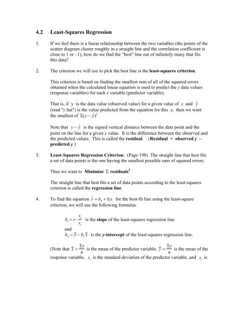
<strong>4.2</strong> <strong>Least</strong>-<strong>Squares</strong> <strong>Regression</strong><br />
1. If we feel there is a linear relationship between the two variables (the points of the<br />
scatter diagram cluster roughly in a straight line and the correlation coefficient is<br />
close to 1 or –1), how do we find the "best" line out of infinitely many that fits<br />
this data<br />
2. The criterion we will use to pick the best line is the least-squares criterion.<br />
This criterion is based on finding the smallest sum of all of the squared errors<br />
obtained when the calculated linear equation is used to predict the y data values<br />
(response variables) for each x variable (predictor variable).<br />
That is, if y is the data value (observed value) for a given value of x and y ˆ<br />
(read "y hat") is the value predicted from the equation for this x, then we want<br />
the smallest of Σ(y − y ˆ ) 2<br />
Note that y − ˆ y is the signed vertical distance between the data point and the<br />
point on the line for a given x value. It is the difference between the observed and<br />
the predicted values. This is called the residual. (Residual = observed y –<br />
predicted y.)<br />
3. <strong>Least</strong>-<strong>Squares</strong> <strong>Regression</strong> Criterion: (Page 198) The straight line that best fits<br />
a set of data points is the one having the smallest possible sum of squared errors.<br />
Thus we want to Minimize Σ residuals 2<br />
The straight line that best fits a set of data points according to the least-squares<br />
criterion is called the regression line.<br />
4. To find the equation ˆ y = b 0<br />
+ b 1<br />
x for the best-fit line using the least-square<br />
criterion, we will use the following formulas.<br />
b 1<br />
= r ⋅ s y<br />
s x<br />
is the slope of the least-squares regression line<br />
and<br />
b 0<br />
= y − b 1<br />
x is the y-intercept of the least-squares regression line.<br />
(Note that x = Σx<br />
Σy<br />
is the mean of the predictor variable, y = is the mean of the<br />
n n<br />
response variable, s x<br />
is the standard deviation of the predictor variable, and s y<br />
is
the standard deviation of the response variable. Also note that<br />
⎛ x i<br />
− x ⎞ ⎛<br />
⎝<br />
⎜<br />
s x<br />
⎠<br />
⎟ y i<br />
− y ⎞<br />
∑ ⎜<br />
⎝ s<br />
⎟<br />
y ⎠<br />
r =<br />
is the correlation coefficient for the data.)<br />
n −1<br />
5. Note that the point (x , y ) is always a point on this least-squares linear regression<br />
line. (This is useful when drawing this line by hand.)<br />
7. Because s x<br />
and s y<br />
are always positive, the sign on the slope of the leastsquares<br />
linear regression line is the same as the sign of the correlation<br />
coefficient r.<br />
8. The slope ( b 1<br />
) can be interpreted as the rate of change of the response variable,<br />
y, with respect to the predictor variable, x. Thus, when x increases by one unit,<br />
y will change by the amount of b 1<br />
.<br />
9. The y-intercept ( b<br />
0<br />
) can be interpreted as the predicted value of the response<br />
variable when the predictor variable is zero. This makes sense only if:<br />
a. The value of 0 for the predictor variable makes sense.<br />
b. There is an observed value of the predictor variable near 0.<br />
10. Never use the least-squares regression line to make predictions for values of<br />
the predictor variable that are much larger or much smaller than the<br />
observed values. (We don't even know if the data far outside our data set would<br />
be linear, much less whether it would follow the same line.)<br />
11. Cautions:<br />
Only use this method when the scatter diagram looks roughly linear. (Also check<br />
the value of r, the correlation coefficient.)<br />
Outliers are data points that lie far from the regression line relative to the other<br />
data points. They can sometimes have a significant effect on the regression<br />
analysis.<br />
12. <strong>Regression</strong> Lines in a Calculator: As was noted in the last section, the<br />
regression line can be found using the calculator. Follow the steps: STAT over<br />
to CALC ENTER (to select #4). Then enter the x-list (say L1), a comma,<br />
and the y-list (say L2) and ENTER. The slope and y-intercept will be given on<br />
2<br />
the screen as well as the r and r values, provided that you have turned on the<br />
Diagnostics.
If you want to store the equation under y<br />
1<br />
(in the Y = key), then you need to<br />
call the y<br />
1<br />
function. To do this follow the steps: VARS over to Y-VARS<br />
ENTER (to select Function) ENTER again (to select y<br />
1<br />
). Thus, the screen<br />
should show: 1-Var Stats L<br />
1<br />
, L<br />
2<br />
, y<br />
1<br />
and then ENTER. The resulting screen<br />
will look the same as it did without the y<br />
1<br />
. But, if you go to the Y = key, the<br />
linear equation will be stored in y<br />
1<br />
. You can then graph the scatter plot and the<br />
regression line by entering ZOOM #9.