12.2 Hypothesis Tests for One Population Proportion
12.2 Hypothesis Tests for One Population Proportion
12.2 Hypothesis Tests for One Population Proportion
Create successful ePaper yourself
Turn your PDF publications into a flip-book with our unique Google optimized e-Paper software.
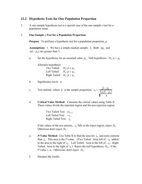
<strong>12.2</strong> <strong>Hypothesis</strong> <strong>Tests</strong> <strong>for</strong> <strong>One</strong> <strong>Population</strong> <strong>Proportion</strong><br />
1. A one-sample hypothesis test is a special case of the one-sample z-test <strong>for</strong> a<br />
population mean.<br />
2. <strong>One</strong>-Sample z-Test <strong>for</strong> a <strong>Population</strong> <strong>Proportion</strong>:<br />
Purpose: To per<strong>for</strong>m a hypothesis test <strong>for</strong> a population proportion, p.<br />
Assumptions: 1. We have a simple random sample. 2. Both<br />
n(1 − p 0<br />
) are greater than 5.<br />
np 0<br />
and<br />
a. Set the hypotheses <strong>for</strong> an assumed value p 0<br />
: Null hypothesis: H 0<br />
: p = p 0<br />
Alternate hypothesis:<br />
Two Tailed: H 0<br />
: p ≠ p 0<br />
Left Tailed: H 0<br />
: p < p 0<br />
Right Tailed: H 0<br />
: p > p 0<br />
b. Significance level: α<br />
c. Test statistic, where ˆ p is the sample proportion: z 0<br />
=<br />
ˆ p − p 0<br />
p 0<br />
(1 − p 0<br />
)<br />
n<br />
d. Critical Value Method: Calculate the critical values using Table II.<br />
These values divide the rejection region and the non-rejection region:<br />
Two Tailed Test: ±z α /2<br />
Left Tailed Test: −z α<br />
Right Tailed Test: z α<br />
If the values of the test statistic,<br />
Otherwise don't reject H 0<br />
.<br />
z 0<br />
falls in the reject region, reject H 0<br />
.<br />
e. P-Value Method: Use Table II to find the area <strong>for</strong> z<br />
0<br />
and more extreme<br />
than z 0<br />
. This area is the P-value. (Two Tailed: Area left of – z 0<br />
added<br />
to the area to the right of z 0<br />
. Left Tailed: Area to the left of – z 0<br />
. Right<br />
Tailed: Area to the right of z 0<br />
.) Reject the null hypothesis, H 0<br />
, if the<br />
P-value ≤ α. Otherwise, don't reject H 0<br />
.<br />
f. Interpret the results.
3. A calculator can also be used to per<strong>for</strong>m this test. Use #5: 1-Prop ZTest under<br />
STAT TESTS.<br />
12.3 Inferences <strong>for</strong> two <strong>Population</strong> <strong>Proportion</strong>s, Using Independent<br />
Samples<br />
1. We will now study a method <strong>for</strong> comparing proportions computed <strong>for</strong> two<br />
populations with one attribute. Are these proportions equal<br />
2. We will use independent random samples from each population to per<strong>for</strong>m a<br />
hypothesis test and to find a confidence interval to determine whether the<br />
proportion of one population with the attribute is equal to the proportion of the<br />
other population with the same attribute.<br />
3. To do this we need to know the distribution of the difference between two sample<br />
proportions.<br />
4. Notation:<br />
<strong>Population</strong> 1 <strong>Population</strong> 2<br />
<strong>Population</strong> <strong>Proportion</strong> p 1<br />
p 2<br />
Sample Size n 1<br />
n 2<br />
Number of Successes x 1<br />
x 2<br />
Sample <strong>Proportion</strong><br />
ˆ p 1<br />
= x 1<br />
n 1<br />
ˆ p 2<br />
= x 2<br />
n 2<br />
5. The Sampling Distribution of the Difference Between Two Sample<br />
<strong>Proportion</strong>s <strong>for</strong> Independent Samples<br />
For independent samples of sizes and from the two populations:<br />
n 1<br />
n 2<br />
µ ˆ p 1 − ˆ p 2<br />
= p 1<br />
− p 2<br />
σ<br />
p ˆ 1 − p ˆ 2<br />
=<br />
p 1<br />
(1 − p 1<br />
)<br />
n 1<br />
+ p 2 (1− p 2 )<br />
n 2<br />
ˆ p 1<br />
− p ˆ 2<br />
is approximately normally distributed <strong>for</strong> large n 1<br />
and n 2<br />
.<br />
6. From the above we see that the standardized variable is<br />
z =<br />
z =<br />
( p ˆ 1<br />
− p ˆ 2<br />
) − ( p 1<br />
− p 2<br />
)<br />
p 1<br />
(1 − p 1<br />
)<br />
+ p 2(1 − p 2<br />
)<br />
n 1<br />
n 2<br />
p ˆ 1<br />
− p ˆ 2<br />
1<br />
p(1 − p) + 1 n 1<br />
n 2<br />
, which if p 1<br />
= p 2<br />
= p becomes
However, since p is not known, we will replace it with the pooled sample<br />
x<br />
proportion ˆ p p<br />
= 1<br />
+ x 2<br />
.<br />
n 1<br />
+ n 2<br />
7. Two-Sample z-Test <strong>for</strong> Two <strong>Population</strong> <strong>Proportion</strong>s:<br />
Purpose: To per<strong>for</strong>m a hypothesis test to compare two population proportions, p 1<br />
and p 2<br />
.<br />
Assumptions: 1. We have a simple random samples that are independent. 2. x 1<br />
,<br />
n 1<br />
− x 1<br />
, x 2<br />
, and n 2<br />
− x 2<br />
, are all greater than 5.<br />
a. Set the hypotheses assuming the population proportions are equal.<br />
Null hypothesis: H 0<br />
: p 1<br />
= p 2<br />
Alternate hypothesis:<br />
Two Tailed: H 0<br />
: p 1<br />
≠ p 2<br />
Left Tailed: H 0<br />
: p 1<br />
< p 2<br />
Right Tailed: H 0<br />
: p 1<br />
> p 2<br />
b. Significance level: α<br />
c. Test statistic: z 0<br />
=<br />
p ˆ 1<br />
− p ˆ 2<br />
ˆ p p<br />
(1 − p ˆ p<br />
)<br />
1<br />
n 1<br />
+ 1 n 2<br />
d. Critical Value Method: Calculate the critical values using Table II.<br />
These values divide the rejection region and the non-rejection region:<br />
Two Tailed Test: ±z α /2<br />
Left Tailed Test: −z α<br />
Right Tailed Test: z α<br />
If the values of the test statistic,<br />
Otherwise don't reject H 0<br />
.<br />
z 0<br />
falls in the reject region, reject H 0<br />
.<br />
e. P-Value Method: Use Table II to find the area <strong>for</strong> z 0<br />
and more extreme<br />
than z 0<br />
. This area is the P-value. (Two Tailed: Area left of – z 0<br />
added<br />
to the area to the right of z 0<br />
. Left Tailed: Area to the left of – z 0<br />
. Right<br />
Tailed: Area to the right of z 0<br />
.) Reject the null hypothesis, H 0<br />
, if the<br />
P-value ≤ α. Otherwise, don't reject H 0<br />
.<br />
f. Interpret the results.
8. Two-Sample z-Interval Procedure: To find a confidence interval <strong>for</strong> the<br />
difference between two population proportions, p 1<br />
and p 2<br />
.<br />
Assumptions: 1. We have a simple random samples that are independent. 2. x 1<br />
,<br />
n 1<br />
− x 1<br />
, x 2<br />
, and n 2<br />
− x 2<br />
, are all greater than 5.<br />
For the confidence level of 1 – α, use Table II to find z α /2<br />
The end points of the confidence interval <strong>for</strong> p 1<br />
– p 2<br />
are<br />
( p ˆ 1<br />
− p ˆ 2<br />
) ± z α /2<br />
⋅<br />
p ˆ 1<br />
(1− p ˆ 1<br />
) p<br />
+ ˆ 2<br />
(1 − p ˆ 2<br />
)<br />
.<br />
n 2<br />
n 1<br />
Interpret the confidence interval.<br />
9. The margin of error <strong>for</strong> the estimate of p 1<br />
– p 2<br />
is<br />
E = z α /2<br />
⋅<br />
p ˆ 1<br />
(1 − p ˆ 1<br />
) p<br />
+ ˆ 2<br />
(1 − p ˆ 2<br />
)<br />
.<br />
n 2<br />
n 1<br />
This is half the length of the confidence interval and it represents the precision<br />
with which ˆ p 1<br />
– ˆ p 2<br />
estimates p 1<br />
– p 2<br />
.<br />
10. Sample Size <strong>for</strong> Estimating p 1<br />
– p 2<br />
: A (1−α)-level confidence interval <strong>for</strong> the<br />
difference between two population proportions that has a margin of error of at<br />
most E can be obtained by choosing<br />
⎛<br />
n 1<br />
= n 2<br />
= 0.5 z α /2 ⎞<br />
⎝ E ⎠<br />
2<br />
rounded up to the nearest whole number.<br />
If you can make educated guesses, ˆ p 1g<br />
and p ˆ 2g<br />
<strong>for</strong> ˆ p 1<br />
and ˆ p 2<br />
, you should<br />
instead choose<br />
n 1<br />
= n 2<br />
=<br />
(<br />
p ˆ 1g<br />
(1 − p ˆ 1g<br />
) + p ˆ 2g<br />
(1− p ˆ 2g<br />
)) ⎛<br />
⎝<br />
z α /2<br />
E<br />
⎞<br />
⎠<br />
2<br />
rounded up to the nearest<br />
whole number. (If a range an estimate <strong>for</strong> ˆ p 1<br />
and ˆ p 2<br />
are given as a range of<br />
values are pick the values in the range that are closest to 0.5.)<br />
11. <strong>Hypothesis</strong> test <strong>for</strong> two population proportions can be conducted with a calculator<br />
using 2-PropZTest under STAT TEST. Confidence intervals can be found in<br />
the calculator using 2-PropZInt under STAT TEST.


