A Method for Fine Registration of Multiple View Range Images ...

Computer Vision and Image Understanding 87, 66–77 (2002) 

doi:10.1006/cviu.2002.0983 

A Method for Fine Registration of Multiple View 

Range Images Considering the Measurement 

Error Properties 

Ikuko Shimizu Okatani 

Department of Information and Computer Sciences, Saitama University Shimo-Okubo 255, 

Saitama, 338-8570, Japan 

E-mail: ikuko@cda.ics.saitama-u.ac.jp 

and 

Koichiro Deguchi 

Graduate School of Information Sciences, Tohoku University Aoba-Campus01, Sendai, 980-8579, Japan 

E-mail: kodeg@fractal.is.tohoku.ac.jp 

Received August 31, 2001; accepted September 6, 2002 

This paper presents a new method for fine registration of two range images from 

different viewpoints that have been roughly registered. Our method deals with the 

properties of the measurement error of the range image data. The error distribution 

is different for each point in the image and is usually dependent on both the viewing 

direction and the distance to the object surface. We find the best transformation 

of two range images to align each measured point and reconstruct 3D total object 

shape by taking such properties of the measurement error into account. The position 

of each measured point is corrected according to the variance and the extent of 

the distribution of its measurement error. The best transformation is selected by 

the evaluation of the effectiveness of this correction of every measured point. The 

experiments showed that our method produced better results than the conventional 

ICP method. c○ 2002 Elsevier Science (USA) 

Key Words: range image; registration; multiple views; measurement error. 

1. INTRODUCTION 

This paper proposes a method for fine registration of range images obtained from several 

different viewpoints to reconstruct the total object shape. Each range image data is represented 

in an individual 3D coordinate system that depends on the position and the orientation 

of the range finder. Hence, to integrate them, the transformations of the coordinate systems 

1077-3142/02 $35.00 

c○ 2002 Elsevier Science (USA) 

All rights reserved. 

66

FINE REGISTRATION OF MULTIPLE VIEW RANGE IMAGES 67 

must be estimated correctly. Many methods for 3D reconstruction by integrating registered 

range images have been proposed [1–3]. To reconstruct a reliable model of the object, an 

algorithm considering the measurement error of the range image data was proposed [3]. 

However, there are some difficulties in fine registration of range images. First, range 

images are given as sets of discrete points, and different sets of range images obtained 

from different viewpoints do not usually include a common object point. Second, some 

areas of an object surface observed from one viewpoint are not observed from the other 

viewpoints because of the occlusion. Before the registration has been done, we cannot know 

which areas are commonly observed. Furthermore, they contain measurement error whose 

properties depend on both the relative orientation of the surface to the viewing direction 

and the distance from the surface to the viewpoint; that is, the properties of measurement 

error are different for each point. 

Several registration methods attempting to overcome these difficulties have been proposed 

in the literature. In those methods, first, rough registration was carried out by selecting 

some feature points and establishing their correspondences between multiple views [4, 5]. 

Next, the iterative closest point (ICP) method proposed by Besl [6] was applied for fine 

registration. Almost all of the subsequent methods for fine registration have been based 

on and extensions of the ICP method. In the ICP method, a point set is registered to 

another point set by minimizing the sum of squared Euclidean distances from each point 

in the first set to the nearest point in the second set. However, the nearest pairs are not 

necessarily the true corresponding ones. This limited the performance of the original ICP 

method. To maintain correspondences, Zhang [7] excluded the corresponding pair whose 

distance is larger than a threshold. Chen [8] and Dorai [9] used only smooth surface parts 

to register the point sets and minimized the sum of distances between each point in one 

image to a tangential plane made from points in another image. Turk [10] represented 

range images as a set of triangular patches and eliminated corresponding pairs of which 

either is on the surface boundary. Masuda [11] employed a robust estimation technique 

also to avoid false correspondences. Bergevin [12] proposed simultaneous registering of 

multiple range images to avoid the accumulation of the errors in the sequential estimation 

of transformations. But, those methods did not achieve fine registration because they did 

not consider the characteristic properties of the measurement error. 

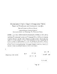
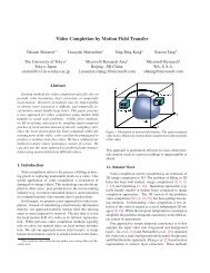
Generally, the measurement errors of distant points and points on a steep surface with 

respect to the viewing direction become larger, as shown in Fig. 1. In addition, the measurement 

error in the viewing direction is much larger than those in the directions parallel to 

the image plane. Therefore, to achieve a fine registration, we must take into account these 

FIG. 1. 

Distributions of measurement errors in range images.

68 OKATANI AND DEGUCHI 

error properties, while the conventional methods based on the ICP method considered these 

errors to be isotropic and uniform at every point. 

In our method, one of the range images will be represented as a set of triangular patches, 

and the other as a set of points. We estimate the most probable transformation of the second 

image to overlay it onto the first image considering the measurement error distributions. 

For a given transformation, the positions of every measured point both in the two range 

images are corrected according to the individual variance of its measurement error. The 

amount and the direction of the correction depend on the extent of the measurement error 

distribution which is expressed the error variance. Then, the best transformation is selected 

by the evaluation of the facility of this correction of all measured points. 

To establish the best registration by this new approach, the problem still remains that we 

do not know which point in the second image must lie on which triangular patch in the first 

image. The true transformation can be estimated after proper correspondences of points and 

patches have been established. For this problem, we employ an alternative iteration of the 

estimations of the transformation and the correspondences. 

In Section 2, we discuss on the properties of the measurement error of the range image. 

Then, we propose a fine registration algorithm in Section 3. Experimental results are shown 

in Section 4. 

2. MEASUREMENT ERROR IN RANGE FINDING 

A range image obtained by a range finder is represented in the coordinate system depending 

on the position and the orientation of the range finder. We denote each coordinate system 

with the x- and y-axes being within the image plane and the z-axis in the viewing direction. 

For a measurement x = (x, y, z) ⊤ of an object point, we assume that its measurement error 

x − ¯x with respect to the true value ¯x is the normal distribution with an expectation of 0 

and the covariance matrix V [ ¯x]. 

Among the factors which cause the measurement error, the image quantization error is 

principal. Generally, as is in stereo, the positional error in the viewing direction which is 

caused by the image quantization will be proportional to the square of the distance, while the 

error in parallel directions to the image plane will be linearly proportional to the distance [13] 

so that the positional error in the z direction is considered to be dominant and the errors in the 

x and y directions can be neglected in registration. Hence, we approximate V [x] as having 

the form V [x] = ( 0 0 0 0 0 

0). This approximation assumes that the distribution of the measurement 

z of the point whose true distance is ¯z is expressed by the probability density 

2 0 0 σ 

function 

[ 

1 

p(z|¯z) = √ exp − 1 ( ) ] 

¯z − z 

2 

, (1) 

2πσ 

2 2 σ 

and the measurements of x and y are considered to be true values. The standard deviation 

σ of the measurement error depends on the distance to the object point and the steepness 

of the object surface around the point with respect to the viewing direction. 

It should be noted that, as shown in Fig. 1, the dominant directions of the error distributions 

are different according to the viewing directions. Although the error model is still kept simple 

by allowing only errors in the z direction, the correction for fine registration becomes rather 

complicated, but it will be worthwhile applying to obtain the dramatically improved results 

shown in the experiments.


For every measurement x, we denote its estimation of the z coordinate by ẑ. That is, 

ˆx = (x, y, ẑ) ⊤ . 

3. REGISTRATION OF TWO RANGE IMAGES 

3.1. Relation between the Coordinate Systems 

Let us denote the 3D coordinates of the mth point in the first range image by x m 1 , and the 

kth point in the second range image in its own coordinate system by x k 2 . The coordinates xk 2 of 

the second range image will be represented in the first coordinate system by a transformation 

T consisting of a rotation matrix R and a translation vector t as T (x k 2 ) = Rxk 2 + t. Then, 

the registration is to determine the true R and t, and, at the same time, obtain the total 3D 

point set free from measurement error. 

3.2. Estimation of the Transformation 

We assume that the object consists of a set of almost smooth surface segments and that the 

surface segments commonly viewed from both viewpoints have sufficiently dense measured 

points. Then, each segment can be represented as a set of triangular patches. If a point in 

one image does not lie on its corresponding triangular patch in the other image even when 

the true transformation is given, it is caused by measurement error in the range finding. In 

this sense, we find the most probable correspondences of points and patches considering 

the above-mentioned properties of measurement error. Of course, by occlusions etc., some 

of the points in one range image have no correspondence in the other image. These points 

must be properly excluded in the estimation process of the transformation described in 

Section 3.3. 

In our method, the first range image is represented as a set of triangular patches {△ m 1 } 

and the second range image is represented as a set of points {x k 2 }. As shown in Fig. 2, 

we assume that the kth point in the second image corresponds to the n(k)th triangular 

patch △ n(k) 

1 ={x n(k) 1 

1 , x n(k) 2 

1 , x n(k) 3 

1 } in the first image; that is, x k 2 is a measurement of a point 

included within △ n(k) 

1 . If the transformation T is correct and the point T (ˆx k 2 ) does not lie on 

△ n(k) 

1 , as shown in Fig. 3, it is the result from their measurement errors. Hence, the positions 

of x k 2 and also xn(k) m 

1 (m = 1, 2, 3) should be corrected to lie on the same plane. The position 

of each point is corrected only in its viewing direction according to the amount of their 

FIG. 2. 

Correspondence of a point in the second range image and a triangular patch in the first range image.


FIG. 3. If the transformation is correct, a point in the second range image and the three vertices of its 

corresponding triangular patch in the first range image must lie on a plane. 

respective variances of the measurement errors. Thus, we obtain the estimations ˆx n(k) m 

1 and 

ˆx k 2 so that T (ˆxk 2 ) and ˆxn(k) m 

1 lie on the same plane. This implies that 

a k ˆx n(k) 1 

1 + b k ˆx n(k) 2 

1 + c k ˆx n(k) 3 

1 = T (ˆx k 2) 

, ak + b k + c k = 1, 0 ≤ a k , b k , c k ≤ 1. (2) 

We consider that the best transformation achieves this relation with the largest probability 

for both estimations ẑ1 m of zm 1 and ẑk 2 of zk 2 . Such a transformation will be obtained by 

minimizing the next log-likelihood function 

J = ∑ m 

1 (ẑm 

( ) 

σ 

m 2 1 − z m ) 2 

∑ 1 (ẑk 

1 + ( ) 

1 k σ 

k 2 2 − z k 2, 

2) 

(3) 

2 

under the constraint of (2), because the distribution of the measurement z is assumed to be 

expressed with the probability function of (1). 

In our strategy, first, we select T as described later and apply it to the points in the second 

image. Then, every point in the second image and the vertex points of its corresponding 

triangular patch in the first image are moved to lie on a plane, respectively, under the 

constraint that point positions can be corrected only in their respective viewing directions. 

Such a correction is not unique, but we select one which minimizes J of (3) for this 

transformation. 

At this time, we have the estimations ẑ1 m of zm 1 and ẑk 2 of zk 2 in J of (3), and we have 

the value of J for a given transformation T . Then, the transformation ˆT that gives the 

minimum value of J among all the possible T is considered to be the best estimation of 

transformation, so that, in the next step, we modify T to reduce the value of J. 

We employ alternative iterations of the first estimation of the correspondence and the 

second estimation of the transformation. It should be noted that three vertex points of a 

triangular patch are also vertex points of their neighboring triangular patches. This implies 

that all triangular patches cannot be modified independently in the first step. It also should 

be noted that every correspondence of a point and a triangular patch cannot be known 

beforehand.


FIG. 4. Determination of the correspondences. (a) For a point in the second range image, its corresponding 

triangular patch in the first range image is selected as the one at the shortest distance along the viewing direction 

of the second range image. (b) If t k is larger than the threshold, the correspondence should be incorrect. 

3.3. Determination of Correspondences 

In the first step of the iteration, for a given transformation T ,wefind the triangular patch 

n(k) 

1 in the first image which is corresponding to the point x k 2 in the second image. Each 

T (x k 2 ) represented in the first coordinate system has an error in the viewing direction of the 

second image. This direction is expressed as v(T ) = R(0, 0, 1) ⊤ . As shown in Fig. 4a, for 

every measured point T (x k 2 ), we search the corresponding triangular patch in the direction 

v(T ). The nearest triangular patch which has a crossing with a viewing line passing at 

T (x k 2 ) and having a direction v(T ) is selected as the corresponding patch. That is, we first 

find minimum t k which satisfies T (x k 2 ) + t kv(T ) = a k x n(k) 1 

1 + b k x n(k) 3 

1 + c k x n(k) 3 

1 , under the 

conditions of (2), and the triangular patch △ n(k) 

1 that gives the minimum t k is determined to 

be the corresponding patch. 

If this minimum value of t k is not small enough, it is considered to be the case shown 

in Fig. 4b, where the correspondence of n(k) is assigned to an incorrect point x k 2 , and we 

exclude such improper correspondences. 

3.4. Calculation of the Criterion 

As mentioned above, to obtain the most probable transformation T , (3) is minimized 

under constraint of (2). In these equations, T , ẑ1 m, ẑk 2 are unknown. 

From (2), we derive 

z2 k − ẑk 2 = A kz k (T ) + ∑ 3 

m=1 Bm k (T )ẑn(k) m 

1 

C k (T ) + ∑ 3 

m=1 Dm k (T , (4) 

)ẑn(k) m 

1 

where the coefficients A k , Bk m (T )(m = 1, 2, 3) etc. in this expression are given as the 

following by denoting the viewing direction of the second image in the first coordinate 

system with v(T ) = (v 1 (T ),v 2 (T ),v 3 (T )) ⊤ and the coordinates of each second image 

point in the first coordinate system with T (x k 2 ) = (x k (T ), y k (T ), z k (T )) ⊤ : 

A k =− ( x n(k) 1 

1 y n(k) 2 

1 − x n(k) 2 

1 y n(k) ) ( 

1 

1 + x 

n(k) 1 

1 y n(k) 3 

1 − x n(k) 3 

1 y n(k) ) 

1 

1 

− ( x n(k) 2 

1 y n(k) 3 

1 − x n(k) 3 

1 y n(k) ) 

2 

1 ,


Bk 1 (T ) = ( x k (T )y n(k) 2 

1 − x n(k) 2 

1 y k (T ) ) − ( x k (T )y n(k) 3 

1 − x n(k) 3 

1 y k (T ) ) 

+ ( x n(k) 2 

1 y n(k) 3 

1 − x n(k) 3 

1 y n(k) ) 

2 

1 , 

Bk 2 (T ) =−( x k (T )y n(k) 1 

1 − x n(k) 1 

1 y k (T ) ) + ( x k (T )y n(k) 3 

1 − x n(k) 3 

− ( x n(k) 1 

1 y n(k) 3 

1 − x n(k) 3 

1 y n(k) ) 

1 

1 , 

Bk 3 (T ) = ( x k (T )y n(k) 1 

1 − x n(k) 1 

1 y k (T ) ) − ( x k (T )y n(k) 2 

1 − x n(k) 2 

+ ( x n(k) 1 

1 y n(k) 2 

1 − x n(k) 2 

1 y n(k) ) 

1 

1 , 

C k (T ) = v 3 (T )A k , 

Dk 1 (T ) =−v 2(T ) ( x n(k) 2 

1 − x n(k) 3 

1 

Dk 2 (T ) = v 2(T ) ( x n(k) 1 

1 − x n(k) 3 

1 

Dk 3 (T ) =−v 2(T ) ( x n(k) 1 

1 − x n(k) 2 

1 

) 

+ v1 (T ) ( y n(k) 2 

1 − y n(k) ) 

3 

1 , 

) 

− v1 (T ) ( y n(k) 1 

1 − y n(k) ) 

3 

1 , 

) 

+ v1 (T ) ( y n(k) 1 

1 − y n(k) 2 

1 

This (4) means that {ẑ2 k} is determined uniquely if {ẑm 1 } is given. 

Using these coefficients, J in (3) is rewritten further as 

J 1 = ∑ m 

1 (ẑm 

( ) 

σ 

m 2 1 − z m ) 2 

∑ 

1 + 

1 k 

1 y k (T ) ) 

1 y k (T ) ) 

[ 

1 A k z k (T ) + ∑ 3 

m=1 

( ) Bm k (T )ẑn(k) m 

1 

σ 

k 2 

2 

) 

. 

C k (T ) + ∑ 3 

m=1 Dm k (T )ẑn(k) m 

1 

] 2 

. (5) 

We estimate the transformation by minimizing J 1 . Then, at this time, the values to be 

estimated are the transformation T and {ẑ m 1 }. 

3.5. Minimization Algorithm 

As described above, we employ alternative iterations of estimations of the transformation 

and point and patch correspondences. This iterative is given as: 

(1) Set initial values for the transformation T 0 . Set c = 0. 

(2) Under the given transformation T c , for every measurement point x k 2 , determine its 

corresponding triangular patch △ n(k) 

1 and obtain a set of correspondences {(k, n(k))} c . 

(3) If all the correspondences are the same as those of the (c − 1)th iteration, consider 

that the algorithm converges and quit. 

(4) Based on the correspondences determined in step 2, estimate {ẑ1 m } and the transformation 

T c by the minimization of J 1 of (5). 

(5) Set the T c+1 with the estimated transformation T c and c = c + 1. Then, return to 

step 2. 

The value of J 1 depends on the transformation and is expressed with its parameters in a rather 

complex form. For the nonlinear minimization done by Newtons method to estimate {ẑ1 m} 

and T c in step 4, we simplify the expression of the transformation by choosing independently 

three parameters to express rotation instead of the rotation matrix R. In our approach, we 

use the three-dimensional vector a, whose direction is just the direction of the rotation axis 

n and whose length is tan(θ/2) where θ is the rotation angle. Then, T (x) can be expressed 

as T (x) = x + 2 (a × x − (a × x) × a) + t. 

1 + a ⊤ a 

By many experiments, we confirmed that this algorithm always converged if sufficiently 

good initial values of T 0 were provided.


4.1. Experiments by Simulation Images 

4. EXPERIMENTS AND DISCUSSIONS 

We intended to conduct performance evaluations of the proposed method, in comparison 

with the conventional ICP registration method, by applying them to two synthetic surfaces 

shown in Fig. 5. 

In the ICP method, first, for every point in the second image, the nearest triangular patch 

in the first image is found. The distance d(T (x k 2 ), n(k) 1 ) from a point of the second image 

to its nearest triangular patch in the first image is usually defined as the shortest Euclidean 

distance to the point included within or on the edge of the triangular patch. Then, the 

transformation is determined so as to minimize the total sum J 2 of the Euclidean distances 

from the transformed points to their corresponding patches. J 2 is given as 

J 2 = ∑ k 

d ( T ( x k 2 

) 

, △ 

n(k) 

1 

) 

. (6) 

To eliminate false corresponding pairs caused by occlusions, corresponding pairs whose 

distances are larger than the threshold or if either of them is on the surface boundary are 

excluded. 

This conventional ICP registration method can be considered a variation of our method 

where the measurement error distribution is assumed to be isotropic around the true point 

position and identical to all the measurements. As described in Section 2, it should be noted 

that these assumptions are not applicable for real range images. 

In Fig. 5, the two arrows above the respective surfaces show the viewing directions 

of the range images. The image sizes were 20 × 20. All the measurements had errors in 

z coordinates depending on their distances from the viewpoint and the steepness of the 

surface around the points. 

We conducted 20 trials of the estimation of the transformation by adding the Gaussian 

measurement errors with mean 0 and variance κεz 2 to all the points (where κ depended on 

the distance and the steepness, and ε was constant). 

The obtained estimation of the errors of the rotation angles and the translation vectors are 

shown in Table 1. They are averages of the absolute values of the errors. The values ε of the 

error variance in the experiments were 0.1 and 0.3. For the surface of (b), the numbers of 

false correspondences were counted for the respective cases where the true transformations 

were given, and the case where they were unknown. The results are shown in Table 2. 

FIG. 5. Synthetic images used for the experiments. The two arrows in the images are the respective viewing 

directions of each image.


TABLE 1 

Estimation of the Errors of the Rotation Angles and Translation Vectors 

ε = 0.1 ε = 0.3 

Average of absolute Average of norm of Average of absolute Average of norm of 

estimation error of translation vector estimation error of translation vector 

rotation angle (degree) error (pixel) rotation angle (degree) error (pixel) 

Surface (a) 

Proposed method 0.13 0.35 0.25 0.44 

ICP method 0.37 0.96 0.36 1.1 

Surface (b) 

Proposed method 0.05 0.41 0.07 0.29 

ICP method 0.71 0.86 1.21 0.97 

As shown in Table 1, the proposed method obtained much higher performances for both 

surfaces. Table 2 shows that the number of false correspondences by the ICP method grew 

so large that the estimation of the transformation did not work well. 

Next, we show the behaviors of the criterion for the transformations. In Fig. 6, the values 

of the criterion J 1 and J 2 obtained around the true transformations are shown in the forms 

of level curves. While the transformation is expressed with six parameters, the figures show 

the values with respect to x and y coordinate displacements from their true values. In Fig. 6, 

(a-·)’s are for the surface of Fig. 5a, and (b-·)’s are for Fig. 5b. (·-1)’s were obtained by the 

proposed method, and (·-2)’s were by the ICP method which did not consider the anisotropy 

of the measurement error. 

As shown in Fig. 6, we confirmed that the criterion J 1 in the proposed method had the minimum 

value at the true transformation, while that of the ICP method had not. This resulted 

from the high ratio of false correspondences in the ICP method as shown in Table 2 even when 

the true transformation was given. In (a-1) and (b-1) of Fig. 6, steep changes of the criterion 

values are found. They resulted from drastic changes of the correspondences at those transformations. 

But the value was monotonically decreasing to the minimum at the true transformation. 

This confirms the convergence of our iterative algorithm proposed in Section 3. 

4.2. Experiments Using Real Range Images 

We applied our method to real range images. Figure 7 shows a wooden hand model used 

in this experiment. Figures 8 and 9 show the results of registration of its range images 

observed from two viewing directions. In those figures, surface points pointed by black and 

white arrows, respectively, were the same positions in both images. In these experiments, 

TABLE 2 

Number and Rate of Correspondence Error 

Number of 

Surface (b) ε = 0.3 Number of points error correspondence Error rate 

Correct transformation Proposed method 400 3.2 0.008 

parameters ICP method 400 103.5 0.26 

Estimated transformation Proposed method 400 8.9 0.022 

parameters ICP method 400 132.7 0.33


FIG. 6. The level curves of the value of the criterion function around the true transformation parameters. 

(a-1) The value of J 1 for the registration of the images in Fig. 5a. (a-2) The value of J 2 for the registration of the 

images in Fig. 5a. (b-1) The value of J 1 for the registration of the images in Fig. 5b. (b-2) The value of J 2 for the 

registration of the images in Fig. 5b. 

FIG. 7. A wooden hand model used for the experiment. The black and white arrows overlaid in the figure 

point to the parts where registrations were drastically improved by our method. (These parts are also pointed to in 

Figs. 8 and 9 with the same arrows.) 

FIG. 8. The registered result of the range images of the hand model. (a) Before registration. (b) After registration. 

Upper and lower images are the same result. Two arrows in the lower figures point to the parts of the 

model which were pointed to by arrows in Fig. 7.


FIG. 9. (a) The triangular patch model generated only from one image and (b) the integrated triangular patch 

model from the two registered images. Two arrows in (b) also point to the same parts of the model which were 

pointed to by arrows in Fig. 7. 

the model of the measurement error was obtained by separate experimental measurements 

using flat plates at several distances and steepness angles. The initial transformation was 

estimated by the feature-based method using the convex hull described in [14]. 

In Fig. 8, the first range image is figured with triangular patches and the second range 

image with points. Figure 8a shows overlay of them before registration, and Fig. 8b is the 

result after registration. Upper and lower figures are the same ones viewed from different 

directions. In the lower figures in Fig. 8, a part of the hand surface pointed to with the white 

arrow and a part of the finger pointed to with the black arrow just fit after the registration. 

Figure 9a shows the first range image expressed with triangular patches, and Fig. 9b 

shows the surface expressed with triangular patches for total registered points of the first 

and the second images after registration. In left side of the hand and a part of a finger, new 

areas of patches were generated. 

5. CONCLUSIONS 

A method for fine registration of roughly registered two range images was proposed. 

Generally, the measurement error of the range image is large for distant object points 

and points on a steep surface with respect to the viewing direction. The measurement error 

is significantly dominant in the viewing direction in comparison with those within the 

image plane. We find the most probable transformation of two range images by taking into 

account such properties of the measurement error. We alternate two steps: the position of 

each measured point is corrected according to the variance and the extent of the distribution 

of each measurement error to align two surfaces for a given transformation, and the best 

transformation of all possible transformations is selected by evaluating the correction. 

The experimental results show that the consideration of the measurement error properties 

as proposed are essential to the estimation of the registration, and this proposed method 

gives much higher accuracies of the registration than the results by the conventional ICP 

method. 

REFERENCES 

1. Y. Chen and G. Medioni, Description of complex objects from multiple range images using an inflating balloon 

model, Comput. Vision Image Understanding 61, 1995, 325–334.


2. M. Soucy and D. Laurendeau, A general surface approach to the integration of a set of range images, IEEE 

Trans. Pattern Anal. Mach. Intell. 17, 1995, 344–358. 

3. A. Hilton, A. J. Stoddart, J. Illingworth, and T. Windeatt, Reliable surface reconstruction from multiple range 

images, in Proceedings of European Conference on Computer Vision, 1996, pp. 117–126. 

4. F. Arman and J. K. Aggarwal, Model-based object recognition in dense-range images—A review, ACM 

Comput. Surv. 25, 1993, 5–43. 

5. O. D. Faugeras and R. Reddy, The representation, recognition, and locating of 3-D objects, Internat. J. Robot. 

Res. 5, 1986, 27–52. 

6. P. J. Besl and N. D. McKay, A method for registration 3-D shapes, IEEE Trans. Pattern Anal. Mach. Intell. 

14, 1992, 239–256. 

7. Z. Zhang, Iterative point matching for registration of free-form curves and surfaces, Internat. J. Comput. 

Vision 13, 1994, 119–152. 

8. Y. Chen and G. Medioni, Object modeling by registration of multiple range images, Image Vision Comput. 

10, 1992, 145–155. 

9. C. Dorai, G. Wang, A. K. Jain, and C. Mercer, Registration and integration of multiple object views for 3D 

model construction, IEEE Trans. Pattern Anal. Mach. Intell. 20, 1998, 83–89. 

10. G. Turk and M. Levoy, Zipped polygon meshes from range images, in ACM SIGGRAPH Computer Graphics, 

1994, pp. 311–318. 

11. T. Masuda and N. Yokoya, A robust method for registration and segmentation of multiple range images, 

Computer Vision Image Understanding 61, 1995, 295–397. 

12. R. Bergevin, D. Laurendeau, and D. Poussart, Registering range views of multipart objects, Comput. Vision 

Image Understanding 61, 1995, 1–16. 

13. J. J. Rodriguez and J. K. Aggarwal, Stochastic analysis of stereo quantization error, IEEE Trans. Pattern Anal. 

Mach. Intell. 12, 1990, 467–470. 

14. I. Shimizu and K. Deguchi, A method to register multiple range images from unknown viewing directions, in 

Proceedings of IAPR Workshop on Machine Vision Applications, 1996, pp. 406–409.

A Method for Fine Registration of Multiple View Range Images ...

You also want an ePaper? Increase the reach of your titles

Delete template?

Save as template?