Gathering light; the telescope - University of Arizona

2.1.Basic Principles
Chapter 2: Gathering light - the telescope
Astronomy centers on the study of vanishingly faint signals, often from complex fields of
sources. Job number one is therefore to collect as much light as possible, with the highest
possible angular resolution. So life is simple. We want to: 1.) build the largest telescope
we can afford (or can get someone else to buy for us), 2.) design it to be efficient and 3.)
at the same time shield the signal from unwanted contamination, 4.) provide diffractionlimited
images over as large an area in the image plane as we can cover with detectors,
and 5.) adjust the final beam to match the signal optimally onto those detectors. Figure
2.1 shows a basic telescope that we might use to achieve these goals.
Achieving
condition 4.) is a
very strong driver
on telescope
design. The
etendue is constant
only for a beam
passing through a
perfect optical
system. For such a
system, the image
Figure 2.1. Simple Prime-Focus Telescope
FoTelescope primary mirror parameters.
quality is limited by the wavelength of the light and the diffraction at the limiting
aperture for the telescope (normally the edge of the primary mirror). Assuming that the
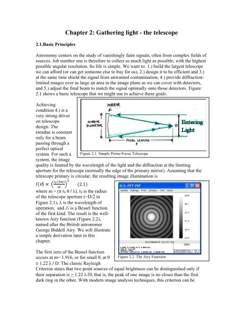
telescope primary is circular, the resulting image illumination is
where m = (π r 0 θ / λ), r 0 is the radius
of the telescope aperture (=D/2 in
Figure 2.1), is the wavelength of
operation, and J 1 is a Bessel function
of the first kind. The result is the wellknown
Airy function (Figure 2.2),
named after the British astronomer
George Biddell Airy. We will illustrate
a simple derivation later in this
chapter.
The first zero of the Bessel function
occurs at m= 1.916, or for small θ, at θ Figure 2.2. The Airy Function
1.22 λ / D. The classic Rayleigh
Criterion states that two point sources of equal brightness can be distinguished only if
their separation is > 1.22 /D; that is, the peak of one image is no closer than the first
dark ring in the other. With modern image analysis techniques, this criterion can be

eadily surpassed. The full width at half maximum of the central image is about 1.03 /D
for an unobscured aperture and becomes slightly narrower if there is a blockage in the
center of the aperture (e.g., a secondary mirror).
Although we will emphasize a more mathematical approach in this chapter, recall from
the previous chapter that the diffraction pattern can be understood as a manifestation of
Fermat’s Principle. Where the ray path lengths are so nearly equal that they interfere
constructively, we get the central image. The first dark ring lies where the rays are out of
phase and interfere destructively, and the
remainder of the light and dark rings represent
constructive and destructive interference at
increasing path differences.
Although the diffraction limit is the ideal, practical
optics have a series of shortcomings, described as
aberrations. There are three primary geometric
aberrations:
1. spherical, occurs when an off-axis input ray is
directed in front of or behind the image
position for an on-axis input
ray, with rays at the same offaxis
angle crossing the image
plane symmetrically
distributed around the on-axis
image. Spherical aberration
tends to yield a blurred halo
around an image (Figure 2.3).
Figure 2.3. The most famous example
of spherical aberration, the Hubble
Space Telescope before various means
were taken to correct the problem.
A sphere forms a perfect Figure 2.4. The focusing properties of a spherical reflector.
image of a point source
located at the center of the sphere, with the image produced on top of the source.
However, for a source at infinity, the distance, F, where the reflected ray crosses the
axis of the mirror is
where R is the radius of curvature of the mirror and is the
angle of reflectance from the surface of the mirror. That is, the
reflected rays cross the mirror axis at smaller values of F the
farther off-axis they impinge on the mirror. The result is
shown in Figure 2.4; there is no point along the optical axis
with a well-formed image.
2. coma occurs when input rays arriving at an angle from the
optical axis miss toward the same side of the on-axis image no
matter where they enter the telescope aperture, and with a
Figure 2.5. Comatic
image displayed to
show interference.

progressive increase in image diameter with increasing distance from the center of the
field. Coma is axially symmetric in the sense that similar patterns are generated by
input rays at the same off axis angle at all azimuthal positions. Comatic images have
characteristic fan or comet-shapes with
the tail pointing away from the center of
the image plane (Figure 2.5).
A paraboloidal reflector provides an
example. The paraboloid by construction
produces a perfect image of a point
source on the axis of the mirror and at
infinite distance. As shown in Figure 2.6,
the focus for a ray that is off-axis by the
angle is displaced from the axis of the
mirror by
3. astigmatism (Figure 2.7) is a cylindrical
wavefront distortion resulting from an
optical system that has different focal
planes for an off-axis object in one
direction from the optical axis of the
system compared with the orthogonal direction. It results in images that are elliptical
on either side of best-focus, with the
direction of the long axis of the ellipse
changing by 90 degrees going from
ahead to behind focus.
Two other aberrations are less fundamental
but in practical systems can degrade the
entendue:
4. curvature of field, which occurs when
the best images are not formed at a
plane but instead on a surface that is
convex or concave toward the telescope
entrance aperture (see Figure 2.8).
Figure 2.6. Focusing properties of a
paraboloidal mirror.
5. distortion arises when the image scale
changes over the focal plane; that is, if a
set of point sources placed on a uniform
grid is observed, their relative image
positions are displaced from the
corresponding grid positions at the focal
plane. Figure 2.9 illustrates symmetric
Figure 2.7. Illustration of astigmatism (from
Starizona). If we assume the astigmatism is
due to an asymmetry in the optics, then the
tangential plane contains both the object being
imaged and the axis of symmetry, and the
sagittal plane is orthogonal to the tangential
one.

forms of distortion, but this defect
can occur in a variety of other forms,
such as trapezoidal.
Neither of these latter two aberrations
actually degrade the images themselves.
The effects of field curvature can be
removed by suitable design of the
following optics, or by curving the
detector surface to match the curvature Figure 2.8. Curvature of field
of field. Distortion can be removed by
resampling the images and placing them at the correct positions, based on a previous
characterization of the distortion effects. Such resampling may degrade the images,
particularly if they are poorly sampled (e.g., the detectors are too large to return all the
information about the images) but need not if care is used both in the system design and
the method to remove the distortion.
Optical systems using lenses are also
subject to:
6. chromatic aberration, resulting
when light of different colors is
not brought to the same focus.
A central aspect of optics design is Figure 2.9. Distortion.
that aberrations introduced by an
optical element can be compensated with a following element to improve the image
quality in multi-element optical systems. For example, some high performance
commercial camera lenses have up to 20 elements that all work together to provide high
quality images over a large field.
In addition to these aberrations, the telescope performance can be degraded by
manufacturing errors that result in the optical elements not having the exact prescribed
shapes, by distortions of the elements in their mountings, and by mis-alignments.
Although these latter effects are also sometimes termed aberrations, they are of a
different class from the six aberrations we have listed and we will avoid this terminology.
In operation, the images can be further degraded by atmospheric seeing, the disturbance
of the wavefronts of the light from the source as they pass through a turbulent atmosphere
with refractive index variations due to temperature inhomogeneity. A rough
approximation of the behavior is that there are atmospheric bubbles of size r 0 = 5 – 15 cm
with temperature variations of a few hundredths up to 1 o C, moving at wind velocities of
10 to 50 m/sec (r 0 is defined by the typical size effective at a wavelength of 0.5m and
called the Fried parameter). The time scale for variations over a typical size of r 0 at the
telescope is therefore of order 10msec. For a telescope with aperture smaller than r 0 , the
effect is to cause the images formed by the telescope to move as the wavefronts are tilted

to various angles by the passage of warmer and cooler air bubbles. If the telescope
aperture is much larger than r 0 , many different r 0 -sized columns are sampled at once.
Images taken over significantly longer than 10msec are called seeing-limited, and have
typical sizes of /r 0 , derived similarly to equation (1.12) since the wavefront is preserved
accurately only over a patch of diameter ~ r 0 . These images may be 0.5 to 1 arcsec in
diameter, or larger under poor conditions. However, since the phase of the light varies
quickly over each r 0 -diameter patch, a complex and variable interference pattern is
formed at the focal plane due to the interference among these different patches. A fast
exposure (e.g., ~ 10msec) freezes this pattern and the image appears speckled, within the
overall envelope of the seeing limit. This behavior is strongly wavelength-dependent.
Because the refractive index of air decreases with increasing wavelength, r 0 increases
roughly as 6/5 , so, for example, the effect of seeing at 10m is largely image motion
even with a 10-m telescope. These topics will be covered more extensively in Chapter 7.
There are a number of ways to describe the imaging performance of a telescope or other
optical system. The nature of the diffraction-limited image is a function of the telescope
configuration (shape of primary mirror, size of secondary mirror, etc.), so we define
“perfect” imaging as that obtained for the given configuration and with all other aspects
of the telescope performing perfectly. The ratio of the signal from the brightest point in
this perfect image divided into the signal from the same point in the achieved image is the
Strehl ratio. We can also measure the ratio of the total energy in an image to the energy
received through a given round aperture at the focal plane, a parameter called the
encircled energy. We can also describe the root-mean-square (rms) errors of the delivered
wavefronts compared with those for the “perfect” image. There is no simple way to relate
these performance descriptors to one another, since they each depend on different aspects
of the optical performance. However, roughly speaking, a telescope can be considered to
be diffraction limited if the Strehl ratio is > 0.8 or the rms wavefront errors are < /14,
where is the wavelength of observation. This relation is known as the Maréchal
criterion. A useful approximate relation between the Strehl ratio, S, and the rms
wavefront error, , is also an extended version of an approximation due to Maréchal:
2.2.Telescope design
We will discuss general telescope design in the context of optical telescopes in the
following two sections, and then in Section 2.4 will expand the treatment to telescopes
for other wavelength regimes. In general, telescopes require the use of combinations of
multiple optical elements. The basic formulae we will use for simple geometric optics can
be found in Section 1.3 (in Chapter 1). For more, consult any optics text.
However, all of these relations are subsumed for modern telescope design into computer
“ray-tracing” programs that follow multiple rays of light through a hypothetical train of
optical elements, applying the laws of refraction and reflection at each surface, to
produce a simulated image. The properties of this image can be optimized iteratively,
with assistance from the program. These programs usually can also include diffraction to
provide a physical optics output in addition to the geometric ray trace.

Nonetheless, there are basic parameters in a telescope and in other optical systems that
you need to understand. We need to define some terms before discussing them:
1. A real image is where the light from an unresolved source is brought to its greatest
concentration – putting a detector at the position of the real image will record the
source.
2. A virtual image can be formed if the optics produce a bundle of light that appears to
come from a real image but no such image has been formed – for example, a convex
mirror may reflect light so it appears that there is a real image behind the mirror.
Except for very specialized applications, refractive telescopes using lenses for their
primary light collectors are no longer employed in astronomy; in addition to chromatic
aberration, large lenses are difficult to support without distortion and they absorb some of
the light rather than delivering it to the image plane (in the infrared, virtually all the light
is absorbed). However, refractive elements are important in other aspects of advanced
telescope design, to be discussed later.
Reflecting telescopes are achromatic and are also efficient because they can be provided
with high efficiency mirror surfaces. From the radio to the near-ultraviolet, metal mirror
surfaces provide reflection efficiencies > 90%, and usually even > 95%. At wavelengths
shorter than ~ 0.15m, metals have poor reflection and multilayer stacks of dielectrics are
used, but with efficiencies of only 50 – 70%. Significantly short of 0.01m (energy > 0.1
keV), grazing incidence reflection can still be used for telescopes, but with significant
changes in configuration as discussed in Section 2.4.4.
Although modern computer-aided optical design would in principle allow a huge
combination of two-mirror telescope systems, the traditional conic-section-based
concepts already work very well. The ability of conic section mirrors to form images is
easily described in terms of Fermat’s Principle. As the surface of a sphere is everywhere
the same distance from its center, so a concave spherical mirror images an object onto
itself when that object is placed at the center of curvature. An ellipse defines the surface
that has a constant sum of the distances from one focus to another, so an ellipsoid images
an object at one focus at the position of its second focus. A parabola can be described as
an ellipse with one focus moved to infinite distance, so a paraboloid images an object at
large distant to its focus. A hyperbola is defined as the locus of points whose difference
of distances from two foci is constant. Thus, a hyperboloid forms a perfect image of a
virtual image.
The basic telescope types based on the properties of these conic sections are:
1. A prime focus telescope (Figure 2.1) has a paraboloidal primary mirror and forms
images directly at the mirror focus; since the images are in the center of the
incoming beam of light, this arrangement is inconvenient unless the telescope is
so large that the detector receiving the light blocks a negligible portion of this
beam

2. A Newtonian telescope (Figure 2.10) uses a flat mirror tilted at 45 o to bring the
focus to the side of the incoming beam of light where it is generally more
conveniently accessed
3. A Gregorian telescope brings the light from its paraboloidal primary mirror to a
focus, and then uses an ellipsoidal mirror beyond this focus to bring it to a second
focus. Usually this light passes through a hole in the center of the primary and the
second focus is conveniently behind the primary and out of the incoming beam.
4. A Cassegrain telescope intercepts the light from its paraboloidal primary ahead of
the focus with a convex hyperboloidal mirror. This mirror re-focuses the light
from the virtual image formed by the primary to a second focus, usually behind
the primary mirror as in the Gregorian design.
Assuming perfect
manufacturing of
their optics and
maintenance of
their alignment,
all of these
telescope types
are limited in
image quality by
the coma due to
their paraboloidal
primary mirrors.
Some less obvious
conic section
combinations are
the Dall-Kirkham,
with an ellipsoidal
primary and
spherical
secondary, and the
inverted Dall-
Kirkham, with a
spherical primary
and ellipsoidal
secondary. Both
suffer from larger
amounts of coma
than for the
paraboloidprimary
types, and
hence they are
seldom used.
Figure 2.10. The basic optical telescope types.

2.3.Matching Telescopes to Instruments
2.3.1. Telescope Parameters
To match the telescope output to an instrument, we need to describe the emergent beam
of light in detail. During the process of designing an instrument, usually an optical model
of the telescope is included in the ray trace of the instrument to be sure that the two work
as expected together. A convenient vocabulary to describe the general matching of the
two is based on the following terms:
The focal length is measured by projecting the conical bundle of rays that arrives at the
focus back until its diameter matches the aperture of the telescope; the focal length is the
length of the resulting projected bundle of rays. See Figure 2.1 for the simplest example.
This definition allows for the effects, for example, of secondary mirrors in modifying the
properties of the ray bundle produced by the primary mirror.
The f-number of the telescope is the diameter of the incoming ray bundle, i.e. the
telescope aperture, divided into the focal length, f/D in Figure 2.1. This term is also used
as a general description of the angle of convergence of a beam of light, in which case it is
the diameter of the beam at some distance from its focus, divided into this distance. The
f-number can also be expressed as 0.5 cotan (θ), where θ is the beam half-angle. Beams
with large f-numbers are “slow” while those with small ones are “fast.”
Equation (1.11) can be used to determine the f-number of the beam at the focus of a
telescope, given the desired mapping of the size of a detector element into its resolution
on the sky. From equation (1.11), we can match to any detector area by adjusting the
optics to shape the beam to an appropriate solid angle. Simplifying to a round telescope
aperture of diameter D and a detector of diameter d,
D d
in
out
Thus, if the detector element is 10m = 1 X 10 -5 m on a side and we want it to map to 0.1
arcsec = 4.85 X 10 -7 rad on the sky on a 10-m aperture telescope, we have
7
5
10m
4.8510
rad 110
m
out
Solving for θ out , the f-number of the beam into the detector is 1.0, a very fast beam
indeed. This calculation previews an issue to be discussed in more detail later, that of
matching the outputs of large telescopes onto modern detector arrays with their relatively
small pixels.
The plate scale is the translation from physical units, e.g. mm, to angular ones, e.g.
arcsec, at the telescope focal plane. As for the derivation of the thin lens formula, we can
determine the plate scale by making use of the fact that any ray passing through telescope
on the optical axis of its equivalent single lens is not deflected. Thus, if we define the
magnification of the telescope, m, to be the ratio of the f number delivered to the focal
plane to the primary mirror f number, then the equivalent focal length of the telescope is
and the angle on the sky corresponding to a distance b at the focal plane is

The field of view (FOV) is the total angle on the sky that can be imaged by the telescope.
It might be limited by the telescope optics and baffles, or by the dimensions of the
detector (or acceptance angle of an instrument).
A stop is a baffle or other construction (e.g., the edge of a mirror) that limits the bundle
of light that can pass through it. Two examples are given below, but stops can be used for
other purposes such as to eliminate any stray light from the area of the beam blocked by
the secondary mirror and other structures in front of the primary mirror.
The aperture stop limits the diameter of the incoming ray bundle from the object. For a
telescope, it is typically the edge of the primary mirror.
A field stop limits the range of angles a telescope can accept, that is, it is the limit on the
telescope field of view.
A pupil is an image of a stop. An entrance pupil is an image of the aperture stop formed
by optics ahead of the stop (not typically encountered with telescopes, but can be used
with other types of optics such as camera lenses or instruments mounted on a telescope).
An exit pupil is an image of the aperture stop formed by optics behind the stop. For
example, the secondary mirror of a Cassegrain (or Gregorian) telescope forms an image
of the aperture stop and hence determines the exit pupil of the telescope. The exit pupil is
often re-imaged within an instrument because it has unique properties for performing a
number of optical functions.
2.3.2. MTF/OTF
The image formed by a telescope
departs from the ideal for
diffraction by a circular aperture
for many reasons, such as: 1.)
non-circular primary mirrors; 2.)
aberrations in the telescope
optics; and 3.) manufacturing
errors. In addition, we need a
convenient way to understand the
combined imaging properties of
the telescope plus instrumentation
being used with it.
The modulation transfer function,
or MTF makes use of the
properties of Fourier transforms
to provide the desired general
description of the imaging
Figure 2.11. Modulation of a signal – (a) input and (b) output.

properties of an optical system. It falls short of a complete description of these properties
because it does not include phase information; the optical transfer function (OTF) is the
MTF times the phase transfer function. However, the MTF is more convenient to
manipulate and is an adequate description for a majority of applications.
To illustrate the meaning of the MTF, imagine that an array of detectors is exposed to a
sinusoidal input signal of period P and amplitude F(x),
where f = 1/P is the spatial frequency, x is the distance along one axis of the array, a 0 is
the mean height (above zero) of the pattern, and a 1 is its amplitude. These terms are
indicated in Figure 2.11a. The modulation of this signal is defined as
where F max and F min are the maximum and minimum values of F(x). We now imagine
that we use a telescope to image a nominally identical sinusoidal pattern onto the detector
array. The resulting output can be represented by
where x and f are the same as in equation above, and b 0 and b 1 (f) are analogous to a 0 and
a 1 (Figure 2.11b). The telescope
will have limited ability to image
very fine details in the sinusoidal
pattern. In terms of the Fourier
transform of the image, this
degradation of the image is
described as an attenuation of the
high spatial frequencies in the
image. The dependence of the
signal amplitude, b 1 , on the spatial
frequency, f, shows the drop in
response as the spatial frequency
grows (i.e., the loss of fine detail in
the image). The modulation in the
image will be
The modulation transfer factor is
Figure 2.12. The MTF (schematically) corresponding to
the function in Figure 2.11b.
A separate value of the MT will apply at each spatial frequency; Figure 2.11a illustrates
an input signal that contains a range of spatial frequencies, and Figure 2.11b shows a
corresponding output in which the modulation decreases with increasing spatial
frequency. This frequency dependence of the MT is expressed in the modulation transfer

function (MTF). Figure 2.12 shows the MTF corresponding to the response of Figure
2.11b.
In principle, the MTF provides a virtually complete specification of the imaging
properties of an optical system. Computationally, the MTF can be determined by taking
the absolute value of the Fourier transform, F(u), of the image of a perfect point source
(this image is called the point spread function). Fourier transformation is the general
mathematical technique used to determine the frequency components of a function f(x)
(see, for example, Press et al. 1986; Bracewell 2000). F(u) is defined as
with inverse
Only a relatively small number of functions have Fourier transforms that are easy to
manipulate. With the use of computers, however, Fourier transformation is a powerful
and very general technique. The Fourier transform can be generalized in a
straightforward way to two dimensions, but for the sake of simplicity we will not do so
here. The absolute value of the transform is
where F*(u) is the complex conjugate of F(u); it is obtained by reversing the sign of all
imaginary terms in F(u).
The point spread function is
the image a system forms
of a perfectly sharp point
input image. If f(x)
represents the point spread
function, |F(u)|/|F(0)| is the
MTF of the system, with u
the spatial frequency. This
formulation holds because a
sharp impulse, represented
mathematically by a
function, contains all
frequencies equally (that is,
its Fourier transform is a
constant). Hence the
Fourier transform of the
image formed from an input
sharp impulse gives the
spatial frequency response
of the optical system.
Figure 2.13. MTF of a round telescope with no central obscuration.
Spatial frequencies are in units of D/λ.

The MTF is normalized to unity at spatial frequency 0 by this definition. As emphasized
in Figure 2.12, the response at zero frequency cannot be measured directly but must be
extrapolated from higher frequencies.
The image of an entire linear optical system is the convolution of the images from each
element. By the "convolution theorem", its MTF can be determined by multiplying
together the MTFs of its constituent elements, and the resulting image is determined by
inverse transforming the resulting MTF. The multiplication occurs on a frequency by
frequency basis, that is, if the first system has MTF 1 (f) and the second MTF 2 (f), the
combined system has MTF(f) = MTF 1 (f) MTF 2 (f). The overall resolution capability of
complex optical systems can be more easily determined in this way than by brute force
image convolution.
We now show the power of the MTF by illustrating the calculation of the Airy function.
We define the box function in two dimensions as
Thus, we describe a round aperture of radius r 0 functionally as
The corresponding MTF is
(see Figure 2.13). The intensity in the image is
This result is identical to equation (2.1) describing the diffraction-limited image.
2.4. Telescope Optimization
2.4.1. Wide Field
The classic telescope designs all rely
on the imaging properties of a
paraboloid, with secondary mirrors to
relay the image formed by the primary
mirror to a second focus. What would
happen if no image were demanded of
the primary, but the conic sections on
the primary and secondary mirrors
were selected to provide optimum
imaging as a unit One answer to this
Figure 2.14. Three-mirror wide field telescope design
after Baker and Paul.
question is the Ritchey-Cretién telescope. In this design, a suitable selection of hyperbolic
primary and secondary together can compensate for the spherical and comatic aberrations

(to third order in an expansion in angle of incidence) and provide large fields, up to an
outer boundary where astigmatism becomes objectionable. An alternative, the aplanatic
Gregorian telescope, has ellipsoidal primary and secondary, and similar wide-field
performance.
Still larger fields can be achieved by adding optics specifically to compensate for the
aberrations. A classic example is the Schmidt camera, which has a full-aperture refractive
corrector in front of its spherical primary mirror. The corrector imposes spherical
aberration on the input beam in the same amount but opposite sign as the aberration of
the primary, producing well-corrected images over a large field. The Maksutov and
Schmidt-Cassegrain designs achieve similar ends with correctors of different types.
However, refractive elements larger than 1 – 1.5m in diameter become prohibitively
difficult to mount and maintain in figure. A variety of designs for correctors near the
focal plane are also possible (e.g., Epps & Fabricant 1997). A simple version invented by
F. E. Ross uses two lenses, one positive and the other negative to cancel each other in
optical power but to correct coma. Wynne (1974) proposed a more powerful device with
three lenses, of positive-negative-positive power and all with spherical surfaces. A
Wynne corrector can correct for chromatic aberration, field curvature, spherical
aberration, coma, and astigmatism. Such approaches are used with all the wide field
cameras on 10-m-class telescopes. These optical trains not only correct the field but also
can provide for spectrally active components, such as compensators for the dispersion of
the atmosphere that allow high quality images to be obtained at off-zenith pointings and
over broad spectral bands (e.g., Fabricant et al. 2004).
Even wider fields can be obtained by adding large reflective elements to the optical train
of the telescope, an approach pioneered by Baker and Paul, see Figure 2.14. The basic
concept is that, by making the second mirror spherical, the light is deviated in a similar
way as it would be by the corrector lens of a Schmidt camera. The third, spherical, mirror
brings the light to the telescope focal plane over a large field. The Baker-Paul concept is a
very powerful one and underlies the large field of the Large Synoptic Survey Telescope
(LSST). . With three or more mirror surfaces to play with, optical designers can achieve a
high degree of image correction in other ways also. For example, a three-mirror
anastigmat is corrected simultaneously for spherical aberration, coma, and astigmatism.
2.4.2. Infrared
The basic optical considerations for groundbased telescopes apply in the infrared as well.
However, in the thermal infrared (wavelengths longer than about 2m), the emission of
the telescope is the dominant signal on the detectors and needs to be minimized to
maximize the achievable signal to noise on astronomical sources. It is not possible to cool
any of the exposed parts of the telescope because of atmospheric condensation. However,
the sky is both colder and of lower emissivity (since one looks in bands where it is
transparent) than the structure of the telescope. Therefore, one minimizes the structure
visible to the detector by using a modest sized secondary mirror (e.g., f/15), matching it
with a small central hole in the primary mirror, keeping the secondary supports and other

structures in the beam with thin cross-sections, and most importantly, removing the
baffles. The instruments operate at cryogenic temperatures; by forming a pupil within
their optical trains and putting a tight stop at it, the view of warm structures can be
minimized without losing light from the astronomical sources. However, the pupil image
generally is not perfectly sharp and the stop is therefore made a bit oversized. To avoid
excess emission from the area around the primary mirror entering the system, often the
secondary mirror is made slightly undersized, so its edge becomes the aperture stop of the
telescope. Only emission from the sky enters the instrument over the edge of the
secondary, and in high-quality infrared atmospheric windows the sky is more than an
order of magnitude less emissive than the primary mirror cell would be.
The emissivity of the telescope mirrors needs to be kept low. If the telescope uses
conventional aluminum coatings, they must be kept very clean. Better performance can
be obtained with silver or gold coatings. Obviously, it is also important to avoid
additional warm mirrors in the optical train other than the primary and secondary.
Therefore, the secondary mirror is called upon to perform a number of functions besides
helping form an image. Because of the variability of the atmospheric emission, it is
desirable to compare the image containing the source with an image of adjacent sky
rapidly, and an articulated secondary can do this in a fraction of a second if desired.
Modulating the signal with the secondary mirror has the important advantage that the
beam passes through nearly the identical column of air as it traverses the telescope (and
even from high into the atmosphere), so any fluctuations in the infrared emission along
this column are common to both mirror positions. A suitably designed secondary mirror
can also improve the imaging, either by compensating for image motion or even
correcting the wavefront errors imposed by the atmosphere (see Chapter 7).
The ultimate solution to these issues is to place the infrared telescope in space, where it
can be cooled sufficiently that it no longer dominates the signals. Throughout the thermal
infrared, the foreground signals can be reduced by a factor of a million or more in space
compared with the ground, and hence phenomenally greater sensitivity can be achieved.
Obviously, space also offers the advantage of being above the atmosphere and hence free
of atmospheric absorption, so the entire infrared range is accessible for observation. The
price of operation in space includes not only cost, but restrictions on the maximum
aperture (being mitigated with JWST), and the inability to change instruments or even to
include all the instrument types desired. Nonetheless, astronomy has benefited from a
series of very successful cryogenic telescopes in space – the Infrared Astronomy Satellite
(IRAS), the Infrared Space Observatory (ISO), the Spitzer Telescope, Akari, the Cosmic
Background Explorer (COBE), and the Wide-Field Infrared Survey Explorer (WISE), to
name some examples.
2.4.3. Radio
Radio telescopes are typically of conventional parabolic-primary-mirror, prime-focus
design. The apertures are very large, so the blockage of the beam by the receivers at the
prime focus is insignificant. The primary mirrors have short focal lengths, f-ratios ~ 0.5,
to keep the telescope compact and help provide a rigid structure. Sometimes the entire

telescope is designed in a way that the flexure as it is pointed in different directions
occurs in a way that preserves the figure of the primary – these designs are described as
deforming homologously. For example, the 100-m aperture Effelsberg Telescope flexes
by up to 6cm as it is pointed to different elevations, but maintains its paraboloidal figure
to an accuracy of ~ 4mm.
Telescopes for the mm- and sub-mm wave regimes are generally smaller and usually are
built in a Cassegrain configuration, often with secondary mirrors that can be chopped or
nutated over small angles to help
compensate for background
emission. They can be
considered to be intermediate in
design between longerwavelength
radio telescopes and
infrared telescopes. Another
exception to the general design
trend is the Arecibo telescope,
which has a spherical primary to
allow steering the beam in
different directions while the
primary is fixed. The spherical
aberration is corrected by optics
near the prime focus of the
telescope in this case.
Radio receivers are uniformly of
coherent detector design; only in
the mm- and sub-mm realms are
bolometers used for continuum
measurements and lowresolution
spectroscopy. The
operation of these devices will Figure 2.15. The Byrd Green Bank Telescope.
be described in more detail in
Chapter 8. For this discussion, we need to understand that all such receivers are limited
by the antenna theorem, which states that they are sensitive only to the central peak of the
diffraction pattern of the telescope, and to only a single polarization.
This behavior modifies how the imaging properties of the telescope are described. The
primary measure of the quality of the telescope optics is beam efficiency, the ratio of the
power from a point source in the central peak of the image to the power in the entire
image. The diffraction rings of the Airy pattern appear to radio astronomers as potential
regions of unwanted sensitivity to sources away from the one at which the telescope is
pointed. This issue is significant because of the relatively low angular resolution and high
sensitivity of single-dish radio telescopes (as opposed to interferometers, see Chapter 9).
The sensitive regions of the telescope beam outside the main Airy peak are called
sidelobes. Additional sidelobes are produced by imperfections in the mirror surface. A

consideration in receiver design is the response over the primary mirror, called the
illumination pattern, to minimize the sidelobes from the image. Sidelobes also arise
through diffraction from structures in the beam, particularly the supports for the primefocus
instruments (or secondary mirror). The Greenbank Telescope (Figure 2.15)
eliminates them with an off-axis primary that brings the focus to the side of the incoming
beam.
2.4.4. X-ray
Certain materials have indices of
refraction in the 0.1 – 10 kev range
that are slightly less than 1 (by ~
0.01 at low energies and only ~
0.0001 at high). Consequently, at
grazing angles these materials
reflect X-rays by total external
reflection; however, at the high
energy end, the angle of incidence
can be only of order 1 o . In addition,
the images formed by grazing
incidence off a paraboloid have
severe astigmatism off-axis, so two
reflections are needed for good
images, one off a paraboloid and
the other off a hyperboloid or
Figure 2.16. A Wolter Type I grazing incidence X-ray
telescope – vertical scale exaggerated for clarity.
ellipsoid. Given these constraints, the optical arrangements of telescopes based on this
type of reflection look relatively familiar (Figure 2.16) – for example, a reflection off a
paraboloid followed by one off a hyperboloid for a Wolter Type-1 geometry (Figure
2.16). A Wolter Type-2 telescope uses a convex hyperboloid for the second reflection to
give a longer focal length and larger image scale, while a Wolter Type-3 telescope uses a
convex paraboloid and concave ellipsoid. The on-axis imaging quality of such telescopes
is strongly dependent on the quality of the reflecting surfaces. The constraints in optical
design already imposed by the grazing incidence reflection make it difficult to correct the
optics well for large fields and the imaging quality degrades significantly for fields larger
than a few arcminutes in radius. The areal efficiency of these optical trains is low, since
their mirrors collect photons only over a narrow annulus. It is therefore common to nest a
number of optical trains to increase the collection of photons without increasing the total
size of the assembled telescope.

As an example, we consider Chandra (Figure 2.17). Its Wolter Type-1 telescope has a
diameter of 1.2m, within which there are four nested optical trains, which together
provide a total collecting area of 1100 cm 2 (i.e., ~ 10% of the total entrance aperture).
Figure 2.17. The Chandra telescope.
The focal length is 10m, the angles of
incidence onto the mirror surfaces range
from 27 to 51 arcmin, and the reflection
material is iridium. The telescope
efficiency is reasonably good from 0.1 to 7
keV. The Chandra design emphasizes
angular resolution. The on-axis images are
0.5 arcsec in diameter (Figure 2.18) but
degrade by more than an order of
magnitude at an off-axis radius of 10
arcmin (Figure 2.19).
The Chandra design can be compared with
that of XMM-Newton, which emphasizes
collecting area. The latter telescope has
three modules of 58 nested optical trains,
Figure 2.18. On-axis image quality for Chandra.
Half of the energy is contained within an image
radius of 0.418 arcsec.
each of diameter 70cm and with a collecting area of 2000cm 2 (~ 50% of the total entrance
aperture). The total collecting area is 6000cm 2 , a factor of five greater than for Chandra.
The range of grazing angles, 18 – 40 arcmin, is smaller than for Chandra resulting in
greater high energy (~ 10 keV) efficiency. The mirrors are not as high in quality as the
Chandra ones, so the on-axis images are an order of magnitude larger in diameter.

For reflecting surfaces,
Chandra and XMM-Newton
used single materials (e.g.,
platinum, iridium, gold) in
grazing incidence. This
approach drops rapidly in
efficiency (or equivalently
works only at more and more
grazing incidence) with
increased energy and is not
effective above about 10 kev.
Higher energy photons can be
reflected using the Bragg
effect. Figure 2.20 shows how
a crystal lattice can reflect by
constructive interference.
With identical layers, the
reflection would be over a
restricted energy range. By
grading multiple layers, broad
Figure 2.19. The Chandra images degrade rapidly with
increasing off-axis angle.
ranges are reflected. The top layers have large spacing (d) and reflect the low energies,
while lower layers have smaller d for higher energies. A stack of up to 200 layers yields
an efficient reflector.
NuStar(to be launched in
2011) uses this approach to
make reflecting optics
working up to 79eV. It will use
a standard Wolter design with
multilayer surfaces deposited
on thin glass substrates,
slumped to the correct shape.
It will have 130 reflecting
shells, with a focal length of
10 meters. The telescope will
be deployed after launch so
the spacecraft fits within the
launch constraints.
Figure 2.20. Bragg Effect. The dots represent the atoms in a
regular crystal lattice. Constructive interference occurs at
specific grazing incidence reflection angles.
2.5.Modern Optical-Infrared Telescopes
2.5.1. 10-meter-class Telescopes

For many years, the Palomar 5-m telescope was considered the ultimate large
groundbased telescope; flexure in the primary mirror was thought to be a serious obstacle
to construction of larger ones. The benefits from larger telescopes were also argued to be
modest. If the image size remains the same (e.g., is set by a constant level of seeing), then
the gain in sensitivity with a background limited detector goes only as the diameter of the
telescope primary mirror.
This situation changed with dual advances. The size limit implied by the 5-m primary
mirror can be violated by application of a variety of techniques to hold the mirror figure
in the face of flexure. The images produced by the telescope can be analyzed to
determine exactly what adjustments are needed to its primary to apply these techniques
and fix any issues with flexure. As a result, the primary can be made both larger than 5
meters in diameter and of substantially lower mass, since the rigidity can be provided by
external controls rather than intrinsic stiffness. In addition, it was realized that much of
the degradation of images due to seeing was occurring within the telescope dome, due to
air currents arising from warm surfaces. The most significant examples were within the
telescope itself – the massive primary mirror and the correspondingly massive steel
structures required to support it and point it accurately. By reducing the mass of the
primary with modern
control methods, the
entire telescope could be
made less massive,
resulting in a
corresponding reduction
in its heat capacity and a
faster approach to
thermal equilibrium with
the ambient temperature.
This adjustment is further
hastened by aggressive
ventilation of the
telescope enclosure,
including providing it
with large vents that
almost place the
telescope in the open air
while observing. The
Figure 2.21. Keck Telescope
gains with the current generation of large telescopes therefore derive from both the
increase in collecting area and the reduction in image size. A central feature of plans for
even larger telescopes is sophisticated adaptive optics systems to shrink their image sizes
further (see Chapter 7).

Three basic approaches have been developed for large groundbased telescopes. The Keck
Telescopes (Figure 2.21), Gran Telescopio Canarias (GTC), Hobby-Everly Telescope
(HET), and South African Large Telescope (SALT) exemplify the use of a segmented
primary mirror. The 10-m primary mirror of Keck is an array of 36 hexagonal mirrors,
each 0.9-m on a side, and made of Zerodur glass-ceramic (this material has relatively low
thermal change with
temperature). The
positions of these
segments relative to
each other are sensed
by capacitive sensors.
A specialized alignment
camera is used to set
the segments in tip and
tilt and then the mirror
is locked under control
of the edge sensors. The
mirrors must be
adjusted very
accurately in piston for
the telescope to operate
in a diffraction-limited
mode. The alignment
camera allows for
adjustment of each pair
of segments in this
coordinate by
Figure 2.22. The MMT.
interfering the light in a small aperture that straddles the edges of the segments. As the
first of the current generation of large telescopes, the Keck Observatory has a broad range
of instrumentation for the optical and near infrared, as well as a high-performance
adaptive optics system.
The VLT, Subaru, and Gemini telescopes use a thin monolithic plate for the optical
element of the primary mirror. We take the VLT as an example – it is actually four
identical examples. They each have 8.2-meter primary mirrors of Zerodur that are only
0.175 meters thick. A VLT primary is supported against flexure by 150 actuators that are
controlled by image analysis at an interval of a couple of times per minute. Again, as a
mature observatory, a wide range of instrumentation is available.
The MMT (Figure 2.22), Magellan, and LBT Telescopes (primaries respectively 6.5, 6.5,
and 8.4m in diameter) are based on a monolithic primary mirror design that is deeply
relieved in the back to reduce the mass and thermal inertia. Use of a polishing lap with a
computer-controlled shape allows the manufacture of very fast mirrors; e.g., the two for
the LBT are f/1.14, which allows an enclosure of minimum size. The LBT is developing
pairs of instruments for the individual telescopes, such as prime focus cameras (with a
red camera at the focus of one mirror and a blue camera for the other), or twin

spectrographs on both sides. The outputs of the two sides of the telescope can also be
combined for operation as an interferometer. The design with the primary mirrors on a
single mount eliminates large path length differences between them and gives the
interferometric applications a uniquely large field of view compared with other
approaches.
2.4.2. Wave Front Sensing
To make the adjustments that maintain their image quality, all of these telescopes depend
on frequent and accurate
measurement of the telescope
aberrations that result from
flexure and thermal drift. A
common way to make these
measurements is the Shack-
Hartmann Sensor, which
operates on the principle
illustrated in Figure 2.23 (see
http://www.wavefrontscience
s.com/Historical%20Develop
ment.pdf for a historical
description). A “perfect”
optical system maintains
wavefronts that are plane or
spherical. In the Shack-
Hartmann Sensor, the
wavefront is divided at a
pupil by an array of small Figure 2.23. Principle of operation of a Shack-Hartmann Sensor.
lenslets. In Figure 2.23, the
situation for a perfect plane wavefront is shown in dashed lines going in to the lenslet
array. Each lenslet images its piece of the wavefront onto the CCD (the imaging process
is shown as the paths of the outer rays, not the wavefronts) directly behind the lens, on its
optical axis. For the plane input wavefront, these images will form a grid that is
uniformly spaced.
Aberrations impose deviations on the wavefronts. An example is shown as a solid line in
Figure 2.23. Each lenslet will see a locally tilted portion of the incoming wavefront, as if
it saw an unaberrated wavefront from the wrong direction. As a result, the images from
the individual lenslets will be tilted relative to the optical axis of the lens and displaced
when they reach the CCD. A simple measurement of the positions of these images can
then be used to calculate the shape of the incoming wavefront, and hence to determine the
aberrations in the optics from which it was delivered. These can be corrected by a
combination of adjustments on the primary mirror and motions of the secondary (e.g., the
latter to correct focus changes).
2.4.3. Telescopes of the Future

The methods developed for control of the figure of large primary mirrors on the ground
have been adopted for the James Webb Space Telescope, in this case so the 6.5-m
primary mirror can be folded to fit within the shroud of the launch rocket. After launch,
the primary is unfolded and then a series of ever more demanding tests and adjustments
will bring it into proper figure. The demands for very light weight have led to a primary
mirror of 18 segments of beryllium, and fast optically (roughly f/1.5, but after reflection
off the convex secondary the telescope has a final f/ratio of about 17). Periodic
measurements with the near infrared camera will be used to monitor the primary mirror
figure and adjust it as necessary for optimum performance. The overall design is a threemirror
anastigmat (meaning it is corrected fully for spherical aberration, coma, and
astigmatism), with a fourth mirror for fine steering of the images.
There are a number of proposals for 30-meter class groundbased telescopes. Given the
slow gain in sensitivity with increasing aperture for constant image diameter, all of these
proposals are based on the potential for further improvements in image quality to
accompany the increase in size. These gains will be achieved with multi-conjugate
adaptive optics (MCAO). MCAO is based on multiple wavefront-correcting mirrors, each
mirror placed in the optics to work at a particular elevation in the atmosphere (or more
accurately, at a given range from the telescope). Laser beacons are directed into the
atmosphere and the returned signals (due, e.g., to scattering) along with those from
natural guide stars are analyzed to determine the corrections to apply to these mirrors.
Such a system achieves a three-dimensional correction of the atmospheric seeing and can
1.) extend the corrections to shorter wavelengths, i.e., the optical; 2.) increase the size of
the compensated field of view; and 3.) improve the uniformity of the images over this
field. See Chapter 7 for additional discussion of MCAO.
One proposal, the Thirty Meter Telescope (TMT), is from a partnership of Canada,
CalTech, the
University of
California, Japan,
China, and India
(some still in
“observer” status).
This telescope would
build on the Keck
Telescope approach.
Its primary mirror
would have 492
segments (up from 36
for Keck). The
European Southern
Observatory
proposed to build a
100-m telescope
called the
Figure 2.24. Artist’s concept of the Giant Magellan Telescope.

Overwhelming Large Telescope (OWL). It was not clear what they would name the next
generation one, so they have scaled down to the European Extremely Large Telescope
(E-ELT), a 42-m aperture segmented mirror design. The Giant Magellan Telescope
(GMT, Figure 2.24) is being developed by an international consortium, including the
University of Arizona plus Astronomy Australia Ltd., the Australian National University,
the Carnegie Institution for Science, Harvard University, the Korea Astronomy and Space
Science Institute, the Smithsonian Institution, Texas A&M University, the University of
Texas at Austin, and the University of Chicago. It will be based on a close-packed
arrangement of seven 8.4-m mirrors, shaped to provide one continuous primary mirror
surface. Its collecting area would be equivalent to a 21-m single round primary.
All of these projects face a number of technical hurdles to work well enough to justify
their cost. We have already mentioned that their sensitivity gains are dependent on the
success of Multi-Conjugate Adaptive Optics. Their large downward looking secondary
mirrors are a challenge to mount, because they have to be “hung” against the pull of
gravity, a much more difficult arrangement than is needed for the upward looking
primary mirrors. For the segmented designs, the electronic control loop to maintain
alignment will be very complex. All of them will be severely challenged by wind, which
can exert huge forces on their immense primary mirrors and structures. Nonetheless, we
can hope that the financial and technical problems will be surmounted and that they will
become a reality.
References
Epps, H. W., & Fabricant, D. 1997, AJ, 113, 439
Fabricant, D. et al. 2004, SPIE, 5492, 767
Wynne, C. G. 1974, MNRAS, 167, 189
Further Reading
Bely, The Design and Construction of Large Optical Telescopes, 2003. Covers
management principles as well as the usual topics in instrumentation.
Bracewell, R. N. 2000, The Fourier Transform and its Applications, 3 rd Ed.
Press, W. H. et al. 2007, Numerical Recipes, 3 rd Ed.
Schroeder, Astronomical Optics, 2 nd edition, 1999. Rather mathematical, but classic
treatment of this topic.
Wilson, Reflecting Telescope Optics, 2 nd ed., 1996; probably more than you wanted to
know