4.1 Quantitative Data Analysis Prof. Treiman Exercise 4: Illustrative ...
4.1 Quantitative Data Analysis Prof. Treiman Exercise 4: Illustrative ...
4.1 Quantitative Data Analysis Prof. Treiman Exercise 4: Illustrative ...

You also want an ePaper? Increase the reach of your titles
YUMPU automatically turns print PDFs into web optimized ePapers that Google loves.
<strong>Quantitative</strong> <strong>Data</strong> <strong>Analysis</strong><br />
<strong>Prof</strong>. <strong>Treiman</strong><br />
<strong>Exercise</strong> 4: <strong>Illustrative</strong> Answer<br />
A. Direct Standardization via Stata<br />
Here is the table called for in the assignment.<br />
Premarital sex is...<br />
Education<br />
< H.S. grad H.S. grad Some coll. College +<br />
Observed percentages<br />
Always wrong 37.4 32.2 26.5 19.7<br />
Almost always wrong 12.1 7.5 8.8 10.0<br />
Sometimes wrong 10.1 16.4 14.7 20.5<br />
Not wrong at all 40.4 43.9 50.0 49.8<br />
Total 100.0 100.0 100.0 100.0<br />
N (99) (214) (238) (239)<br />
Percentages adjusted for age<br />
Always wrong 25.8 31.4 26.4 19.5<br />
Almost always wrong 15.8 6.9 10.2 10.4<br />
Sometimes wrong 10.3 16.2 15.3 20.8<br />
Not wrong at all 48.1 45.5 48.1 49.3<br />
The top panel of the table shows a modest association between education and attitudes regarding<br />
premarital sex, with the better educated less likely to think that premarital sex is wrong. About<br />
37 per cent of those lacking high school education think that premarital sex is always wrong,<br />
compared to less than 20 per cent of those with college degrees. At the other extreme, only<br />
about 40 per cent of those with less than high school think that premarital sex is not wrong at all<br />
compared to about half of those with at least some college.<br />
We might suspect that these results simply reflect the tendency of older people both to be more<br />
poorly educated and to have less liberal attitudes regarding premarital sex than younger people.<br />
Indeed, both of these associations hold for late 20 th century Americans. [I have estimated but<br />
<strong>4.1</strong>
have not presented the tables, but you can easily make them. In a full analysis, you would want<br />
to show these tables.] But standardizing for age reveals that the association between education<br />
and acceptance of premarital does not arise simply from their joint dependence on age. Indeed,<br />
standardizing for age has virtually no impact on the coefficients in the table, except for those<br />
with less than a high school education—the disapproval of premarital sex by those with less than<br />
a high school education is apparently due in part to the fact that the poorly educated are<br />
disproportionately elderly since there is a noticeable shift toward greater acceptance of<br />
premarital sex in this group after standardizing for age.<br />
The -do- file that created these computations is shown in the Appendix.<br />
B. Simple Correlation and Regression<br />
1. Correlation ratios<br />
a) Table 1A shows a strong relationship between religious affiliation and tolerance of those<br />
opposed to religion, among Americans queried in 1974. Nearly three quarters of the<br />
Jews, nearly two thirds of those without religion, but only two fifths of the Catholics and<br />
hardly more than a quarter of the Protestants are in the highest tolerance category,<br />
endorsing the right of those “against religion” to speak at a public meeting, teach in a<br />
college or university, and have their books included in public library collections.<br />
b) On a three point tolerance scale (the number of endorsements of the rights mentioned in<br />
answer to (1a)), the means (and standard deviations) for the four religious categories are<br />
as follows:<br />
Mean<br />
S.D.<br />
Protestants 1.44 1.40<br />
Catholics 1.83 1.36<br />
Jews 2.36 1.30<br />
No religion 2.34 1.21<br />
Total 1.63 1.42<br />
From visual inspection ("eye balling the data") we are led to a similar conclusion from<br />
the means as from the percentage distributions. Jews and those without religion are<br />
substantially more tolerant than are Catholics, who are in turn substantially more tolerant<br />
than are Protestants.<br />
c. The correlation ratio, 0 2 , is a measure of the ratio of the sum of squared standard deviations<br />
of observations from subgroup means (the within-group sum of squares) to the sum of<br />
squared deviations of observations from the grand mean for the entire sample. It tells us<br />
what proportion of the variance in the dependent variable can be explained by knowledge of<br />
4.2
which of several categories of the independent variable an observation falls into. In the<br />
present case, the correlation ratio tells us how much of the variance in tolerance of antireligionists<br />
we can explain by knowing the religious affiliation of respondents. The easiest<br />
way to compute 0 2 is to compute sums of squares separately for each subgroup and then add<br />
them up to find the “within group sum of squares.” Then compute the sum of squares for the<br />
total column. This, obviously, is the “total sum of squares.” Then simply make the<br />
computation indicated in the assignment. Recall from the assignment that:<br />
2<br />
η = 1−<br />
Within group sum of squares<br />
Total sum of squares<br />
This can be tabulated by hand. But it is possible to exploit Stata to shorten your hand<br />
computations and improve the accuracy. The trick is to read the data into Stata, treating the<br />
tolerance score, the frequencies for each religious group, and the total frequency as variables<br />
and the four rows (excluding the total) as observations. The -do- file I used to get the<br />
correlation ratio is shown as the second section of the Appendix.<br />
For this problem, 0 2 = .056. This indicates that about six per cent of the variance in tolerance<br />
of anti-religionists can be accounted for by the religious affiliations of the population. The<br />
apparent inconsistency between the small percentage of variance explained by religious<br />
affiliation and the large differences in the tolerance levels of the religious groups indicated<br />
by the percentage tables is due to the fact that the more tolerant groups, Jews and those<br />
without religion, are very small, and hence cannot contribute much to the total variance in<br />
the population. Put differently, religious affiliation cannot explain much of the variance in<br />
tolerance because most people have the same religion (65 per cent of the sample is<br />
Protestant). This is an important point, which will recur repeatedly in our subsequent<br />
discussion. Be sure you understand it.<br />
2. Correlation and regression<br />
The Stata do file that generates the output for Part B.2 of the exercise is shown as the third<br />
section of the Appendix. I have extensively documented my do file.<br />
2.a.<br />
2.b.<br />
See the do file.<br />
See the do file.<br />
2.b.1. As we see from the R-squared, 15.9 per cent of the variance in income is explained by<br />
variance in education.<br />
2.b.2. To get predicted levels of income for particular levels of education, we substitute the<br />
level of education into the equation:<br />
4.3
For high school graduates: = - 24,846 + 5141(12) = 36,846<br />
For someone with a B.A.: = - 24,846 + 5141(16) = 57,410<br />
For someone with 4 years after B.A.: = - 24,846 + 5141(20) = 77,974<br />
Yˆ<br />
Yˆ<br />
Yˆ<br />
2.c.<br />
2.d.<br />
2.e.<br />
The correlation ratio is .188. This is three percentage points larger than the squared<br />
product moment correlation (.159). The correlation ratio will always be larger (or, at the<br />
limit, equal to) the squared product moment correlation, since the squared product<br />
moment correlation gives 1 minus the ratio of the sum of squared deviations around a<br />
straight regression line to the sum of squared deviations around the mean of the<br />
dependent variable while the correlation ratio gives 1 minus the ratio of the sum of<br />
squared deviations around the subgroup means to the sum of squared deviations around<br />
the mean of the dependent variable. Recall from your elementary statistics course that<br />
the mean is the point that minimizes the sum of squared deviations. If the means do not<br />
increase in an exactly linear fashion, the sum of squares around the subgroup means<br />
necessarily will be smaller than the sum of squares around the regression line.<br />
See the do file.<br />
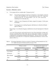
The graph is shown as Fig. 1. The relationship between education and income appears to<br />
be curvilinear. First, no one (in these data) has negative income and so the points for<br />
those with little education are uniformly above the regression line (although we should be<br />
cautious since there are relatively few cases in this part of the graph; very few men in the<br />
sample have less than 8 years of schooling). 1 [I know this not only from inspecting the<br />
scatter plot but also from a tabulation of education that I made but haven’t shown; see the<br />
do file. In the course of your work, you should make many such tabulations to check<br />
whether the data are behaving as expected, even if you never include them in your final<br />
paper.] Second, it is probable that the presence of very high (arbitrarily coded at<br />
$130,000) incomes among some of those with high amounts of education would pull the<br />
line up on the right side were it not constrained to be linear. A better fit to the data might<br />
be found by positing a curvilinear relationship between education and income, which we<br />
will learn how to do shortly. The relatively large variance in income at each level of<br />
education tells us why the squared correlation is so low: while average income tends to<br />
increase with education, there is a great deal of individual variation in the incomes of<br />
equally well educated men. Note finally that the mean for those with 19 years of school<br />
is higher than for those with 20 or more years of school, which probably reflects the fact<br />
that lawyers are better paid than professors.<br />
1 When estimating correlation ratios, one should be cautious about the possibility of “over-fitting” the data<br />
by capitalizing on sampling variation. When the subgroups are small, the subgroup means may reflect sampling<br />
variability rather than true non-linearity in the population. Because of the danger of over-fitting data, it usually is<br />
preferable to estimate r 2 rather than 0 2 when both variables are measured at the interval level—or to fit a smooth<br />
curve if the relationship is curvilinear. An alternative is to collapse small categories into a single larger category. In<br />
the present case, each year of schooling less than eight has fewer than 10 cases, so the estimated means are highly<br />
subject to sampling variability. I might, therefore, have collapsed years 0-8 into a single category to get a more<br />
reliable estimate of the mean for this group.<br />
4.4
3. Individual and aggregate correlations<br />
I ˆ = a+<br />
b ( E )<br />
3.a. We wish to estimate an equation of the form where I = the mean annual<br />
income of white males in each occupation and E = the years of schooling of white males<br />
in each occupation. Our problem is to solve for a and b. We get these from Table 2 by<br />
making use of the relationship and the<br />
b = r ( s / s ) = .72(2153/ 2.3) = 674<br />
YX YX Y X<br />
Y = a+ b( X)<br />
a = Y −b( X)<br />
relationship , which implies that . Thus, a = 5,311 -<br />
674(10.2) = -1,564.<br />
2<br />
3.b. r = .72 2 IE<br />
= .5184. So 52 per cent of the variance over occupations in mean annual<br />
income can be attributed to variance in the average years of school completed by<br />
incumbents.<br />
3.c.<br />
Recall from Part 2 that 16 per cent of the variance in the income of individuals can be<br />
explained by variance in their education, compared to 52 per cent of the variance in the<br />
average income of occupations explained by variance in their average income. It will<br />
almost always be the case that aggregated data will show higher correlations than<br />
disaggregated data involving the same variables, because most of the random<br />
variability is removed when summary characteristics of central tendency (medians,<br />
means, per cent above a certain level, etc.) are correlated. Be sure you understand this<br />
point. In the present case, this is easy to see by thinking about specific occupations. For<br />
example, while an occasional truck driver might be well educated and a few truck drivers<br />
(not necessarily the well educated ones) might make a good deal of money, truck drivers<br />
on the whole neither are very well educated nor make much money.<br />
4.5
150000<br />
Observed<br />
Linear fit<br />
Mean|Yrs. of School<br />
Annual Income in 1993<br />
100000<br />
50000<br />
0<br />
0 4 8 12 16 20<br />
Years of Schooling<br />
Fig. 1. Annual Income in 2003 by Years of School Completed, U.S. Males, 2004 (Open-ended<br />
Upper Category Coded to $150,000); N=855.<br />
Appendix - Log File for the Computations<br />
--------------------------------------------------------------------------------------<br />
log: d:\teach\soc212ab\2007-2008\computing\ex05.log<br />
log type: text<br />
opened on: 2 Nov 2007, 22:07:26<br />
. version 10.0<br />
. #delimit;<br />
delimiter now ;<br />
. clear;<br />
. set more 1;<br />
. program drop _all;<br />
. set mem 100m;<br />
Current memory allocation<br />
current<br />
memory usage<br />
settable value description (1M = 1024k)<br />
--------------------------------------------------------------------<br />
set maxvar 5000 max. variables allowed 1.909M<br />
set memory 100M max. data space 100.000M<br />
set matsize 500 max. RHS vars in models 1.949M<br />
-----------<br />
103.858M<br />
. *EX05.DO (DJT 8/31/03, last modified 11/2/06);<br />
4.6
. ***********************************************<br />
> This -do- file does the computations for Ex. 5.<br />
> ***********************************************;<br />
. ********************************<br />
> *Part A: Direct standardization.<br />
> ********************************;<br />
. use c:\e_old\data\gss\gssy2004.dta,replace;<br />
. *Create a categorical variable for education.;<br />
. recode educ<br />
> (0/11=1 "Some H.S. or less")<br />
> (12=2 "H.S. grad")<br />
> (13/15=3 "Some college")<br />
> (16/20=4 "Coll.grad.or more")<br />
> (*=.),gen(edcat) label(edcat);<br />
(2809 differences between educ and edcat)<br />
. *Create a categorical variable for age.;<br />
. recode age<br />
> (25/34=1 "25-34")<br />
> (35/44=2 "35-44")<br />
> (45/54=3 "45-54")<br />
> (55/64=4 "55-64")<br />
> (65/89=5 "65+")<br />
> (*=.),gen(agecat) label(agecat);<br />
(2803 differences between age and agecat)<br />
. *Convert the missing data codes for premarital sex to the Stata missing<br />
> value.;<br />
. recode premarsx 0 8 9=.;<br />
(premarsx: 18 changes made)<br />
. tab premarsx;<br />
sex before |<br />
marriage | Freq. Percent Cum.<br />
-----------------+-----------------------------------<br />
always wrong | 238 26.95 26.95<br />
almst always wrg | 79 8.95 35.90<br />
sometimes wrong | 157 17.78 53.68<br />
not wrong at all | 409 46.32 100.00<br />
-----------------+-----------------------------------<br />
Total | 883 100.00<br />
. *Mark the "good"--that is, non-missing--data to ensure that all<br />
> analysis is based on the same data set.;<br />
. mark good if premarsx~=. & agecat~=. & edcat~=.;<br />
. *Get the necessary cross-tabs to understand the relationships among<br />
> the three variables.;<br />
. tab premarsx edcat if good==1,col;<br />
4.7
+-------------------+<br />
| Key |<br />
|-------------------|<br />
| frequency |<br />
| column percentage |<br />
+-------------------+<br />
| RECODE of educ (highest year of school<br />
sex before |<br />
completed)<br />
marriage | Some H.S. H.S. grad Some coll Coll.grad | Total<br />
-----------------+--------------------------------------------+----------<br />
always wrong | 37 69 63 47 | 216<br />
| 37.37 32.24 26.47 19.67 | 27.34<br />
-----------------+--------------------------------------------+----------<br />
almst always wrg | 12 16 21 24 | 73<br />
| 12.12 7.48 8.82 10.04 | 9.24<br />
-----------------+--------------------------------------------+----------<br />
sometimes wrong | 10 35 35 49 | 129<br />
| 10.10 16.36 14.71 20.50 | 16.33<br />
-----------------+--------------------------------------------+----------<br />
not wrong at all | 40 94 119 119 | 372<br />
| 40.40 43.93 50.00 49.79 | 47.09<br />
-----------------+--------------------------------------------+----------<br />
Total | 99 214 238 239 | 790<br />
| 100.00 100.00 100.00 100.00 | 100.00<br />
. tab premarsx agecat if good==1,col;<br />
+-------------------+<br />
| Key |<br />
|-------------------|<br />
| frequency |<br />
| column percentage |<br />
+-------------------+<br />
sex before |<br />
RECODE of age (age of respondent)<br />
marriage | 25-34 35-44 45-54 55-64 65+ | Total<br />
-----------------+-------------------------------------------------------+----------<br />
always wrong | 41 49 38 33 55 | 216<br />
| 22.78 25.39 24.84 27.05 38.73 | 27.34<br />
-----------------+-------------------------------------------------------+----------<br />
almst always wrg | 11 14 13 11 24 | 73<br />
| 6.11 7.25 8.50 9.02 16.90 | 9.24<br />
-----------------+-------------------------------------------------------+----------<br />
sometimes wrong | 31 29 23 20 26 | 129<br />
| 17.22 15.03 15.03 16.39 18.31 | 16.33<br />
-----------------+-------------------------------------------------------+----------<br />
not wrong at all | 97 101 79 58 37 | 372<br />
| 53.89 52.33 51.63 47.54 26.06 | 47.09<br />
-----------------+-------------------------------------------------------+----------<br />
Total | 180 193 153 122 142 | 790<br />
| 100.00 100.00 100.00 100.00 100.00 | 100.00<br />
. tab agecat edcat if good==1,row;<br />
+----------------+<br />
| Key |<br />
|----------------|<br />
| frequency |<br />
| row percentage |<br />
+----------------+<br />
4.8
RECODE of |<br />
age (age |<br />
of | RECODE of educ (highest year of school<br />
respondent |<br />
completed)<br />
) | Some H.S. H.S. grad Some coll Coll.grad | Total<br />
-----------+--------------------------------------------+----------<br />
25-34 | 22 32 57 69 | 180<br />
| 12.22 17.78 31.67 38.33 | 100.00<br />
-----------+--------------------------------------------+----------<br />
35-44 | 16 61 71 45 | 193<br />
| 8.29 31.61 36.79 23.32 | 100.00<br />
-----------+--------------------------------------------+----------<br />
45-54 | 7 39 48 59 | 153<br />
| 4.58 25.49 31.37 38.56 | 100.00<br />
-----------+--------------------------------------------+----------<br />
55-64 | 19 32 38 33 | 122<br />
| 15.57 26.23 31.15 27.05 | 100.00<br />
-----------+--------------------------------------------+----------<br />
65+ | 35 50 24 33 | 142<br />
| 24.65 35.21 16.90 23.24 | 100.00<br />
-----------+--------------------------------------------+----------<br />
Total | 99 214 238 239 | 790<br />
| 12.53 27.09 30.13 30.25 | 100.00<br />
. *Convert the premarital sex variable to a set of dichotomous variables,<br />
> necessary to get directly standardized percentages.;<br />
. tab premarsx if good==1,gen(pm);<br />
sex before |<br />
marriage | Freq. Percent Cum.<br />
-----------------+-----------------------------------<br />
always wrong | 216 27.34 27.34<br />
almst always wrg | 73 9.24 36.58<br />
sometimes wrong | 129 16.33 52.91<br />
not wrong at all | 372 47.09 100.00<br />
-----------------+-----------------------------------<br />
Total | 790 100.00<br />
. *Create the "popvar" variable, here called "tot," required by Stata's<br />
> "dstdize" command. Note that the way to make dstdize work on unit<br />
> rather than tabular data is to set the popvar variable = 1 for each<br />
> case.;<br />
. gen tot=1 if good==1;<br />
(2022 missing values generated)<br />
. *Do the direct standardization.;<br />
. for num 1/4:dstdize pmX tot agecat if good==1,by(edcat);<br />
-> dstdize pm1 tot agecat if good==1,by(edcat)<br />
----------------------------------------------------------<br />
-> edcat= 1<br />
-----Unadjusted----- Std.<br />
Pop. Stratum Pop.<br />
Stratum Pop. Cases Dist. Rate[s] Dst[P] s*P<br />
----------------------------------------------------------<br />
25-34 22 4 0.222 0.1818 0.228 0.0414<br />
35-44 16 2 0.162 0.1250 0.244 0.0305<br />
45-54 7 0 0.071 0.0000 0.194 0.0000<br />
55-64 19 9 0.192 0.4737 0.154 0.0732<br />
65+ 35 22 0.354 0.6286 0.180 0.1130<br />
----------------------------------------------------------<br />
4.9
Totals: 99 37 Adjusted Cases: 25.6<br />
Crude Rate: 0.3737<br />
Adjusted Rate: 0.2581<br />
95% Conf. Interval: [0.1878, 0.3284]<br />
----------------------------------------------------------<br />
-> edcat= 2<br />
-----Unadjusted----- Std.<br />
Pop. Stratum Pop.<br />
Stratum Pop. Cases Dist. Rate[s] Dst[P] s*P<br />
----------------------------------------------------------<br />
25-34 32 9 0.150 0.2813 0.228 0.0641<br />
35-44 61 21 0.285 0.3443 0.244 0.0841<br />
45-54 39 13 0.182 0.3333 0.194 0.0646<br />
55-64 32 6 0.150 0.1875 0.154 0.0290<br />
65+ 50 20 0.234 0.4000 0.180 0.0719<br />
----------------------------------------------------------<br />
Totals: 214 69 Adjusted Cases: 67.1<br />
Crude Rate: 0.3224<br />
Adjusted Rate: 0.3136<br />
95% Conf. Interval: [0.2507, 0.3765]<br />
----------------------------------------------------------<br />
-> edcat= 3<br />
-----Unadjusted----- Std.<br />
Pop. Stratum Pop.<br />
Stratum Pop. Cases Dist. Rate[s] Dst[P] s*P<br />
----------------------------------------------------------<br />
25-34 57 16 0.239 0.2807 0.228 0.0640<br />
35-44 71 18 0.298 0.2535 0.244 0.0619<br />
45-54 48 11 0.202 0.2292 0.194 0.0444<br />
55-64 38 12 0.160 0.3158 0.154 0.0488<br />
65+ 24 6 0.101 0.2500 0.180 0.0449<br />
----------------------------------------------------------<br />
Totals: 238 63 Adjusted Cases: 62.8<br />
Crude Rate: 0.2647<br />
Adjusted Rate: 0.2640<br />
95% Conf. Interval: [0.2062, 0.3218]<br />
----------------------------------------------------------<br />
-> edcat= 4<br />
-----Unadjusted----- Std.<br />
Pop. Stratum Pop.<br />
Stratum Pop. Cases Dist. Rate[s] Dst[P] s*P<br />
----------------------------------------------------------<br />
25-34 69 12 0.289 0.1739 0.228 0.0396<br />
35-44 45 8 0.188 0.1778 0.244 0.0434<br />
45-54 59 14 0.247 0.2373 0.194 0.0460<br />
55-64 33 6 0.138 0.1818 0.154 0.0281<br />
65+ 33 7 0.138 0.2121 0.180 0.0381<br />
----------------------------------------------------------<br />
Totals: 239 47 Adjusted Cases: 46.7<br />
Crude Rate: 0.1967<br />
Adjusted Rate: 0.1952<br />
95% Conf. Interval: [0.1438, 0.2466]<br />
Summary of Study Populations:<br />
edcat N Crude Adj_Rate Confidence Interval<br />
--------------------------------------------------------------------------<br />
1 99 0.373737 0.258100 [ 0.187773, 0.328426]<br />
2 214 0.322430 0.313598 [ 0.250660, 0.376536]<br />
3 238 0.264706 0.263981 [ 0.206202, 0.321759]<br />
4 239 0.196653 0.195220 [ 0.143805, 0.246635]<br />
-> dstdize pm2 tot agecat if good==1,by(edcat)<br />
<strong>4.1</strong>0
[Log omitted for pm2-pm4 to save space.]<br />
. *****************************<br />
> Part B.1: Correlation ratios.<br />
> *****************************;<br />
. preserve;<br />
. *Read in the frequencies from Table 1 in the assignment and confirm correct.;<br />
. clear;<br />
. infile score p c j n tot using ex6b.raw;<br />
(4 observations read)<br />
. list;<br />
+-----------------------------------+<br />
| score p c j n tot |<br />
|-----------------------------------|<br />
1. | 3 265 151 32 65 513 |<br />
2. | 2 212 93 3 18 326 |<br />
3. | 1 155 50 2 5 212 |<br />
4. | 0 322 82 7 13 424 |<br />
+-----------------------------------+<br />
. *Get the within-group sum of squared deviations.;<br />
. for var p c j n: sum score [aw=X] \ gen sdX=X*((score-r(mean))^2)<br />
> \ gen ssX=sum(sdX);<br />
-> sum score [aw=p]<br />
Variable | Obs Weight Mean Std. Dev. Min Max<br />
-------------+-----------------------------------------------------------------<br />
score | 4 954 1.440252 1.403347 0 3<br />
-> gen sdp=p*((score-r(mean))^2)<br />
-> gen ssp=sum(sdp)<br />
-> sum score [aw=c]<br />
Variable | Obs Weight Mean Std. Dev. Min Max<br />
-------------+-----------------------------------------------------------------<br />
score | 4 376 1.832447 1.355896 0 3<br />
-> gen sdc=c*((score-r(mean))^2)<br />
-> gen ssc=sum(sdc)<br />
-> sum score [aw=j]<br />
Variable | Obs Weight Mean Std. Dev. Min Max<br />
-------------+-----------------------------------------------------------------<br />
score | 4 44 2.363636 1.304791 0 3<br />
-> gen sdj=j*((score-r(mean))^2)<br />
-> gen ssj=sum(sdj)<br />
-> sum score [aw=n]<br />
<strong>4.1</strong>1
Variable | Obs Weight Mean Std. Dev. Min Max<br />
-------------+-----------------------------------------------------------------<br />
score | 4 101 2.336634 1.208083 0 3<br />
-> gen sdn=n*((score-r(mean))^2)<br />
-> gen ssn=sum(sdn)<br />
. egen wgss=rsum(ssp ssc ssj ssn) in 4;<br />
(3 missing values generated)<br />
. *Get the total sum of squared deviations.;<br />
. sum score [aw=tot];<br />
Variable | Obs Weight Mean Std. Dev. Min Max<br />
-------------+-----------------------------------------------------------------<br />
score | 4 1475 1.629153 1.416017 0 3<br />
. gen gmean=r(mean);<br />
. for var p c j n: gen tdX=X*((score-gmean)^2) \ gen tsX=sum(tdX);<br />
-> gen tdp=p*((score-gmean)^2)<br />
-> gen tsp=sum(tdp)<br />
-> gen tdc=c*((score-gmean)^2)<br />
-> gen tsc=sum(tdc)<br />
-> gen tdj=j*((score-gmean)^2)<br />
-> gen tsj=sum(tdj)<br />
-> gen tdn=n*((score-gmean)^2)<br />
-> gen tsn=sum(tdn)<br />
. egen tss=rsum(tsp tsc tsj tsn) in 4;<br />
(3 missing values generated)<br />
. *Get eta-squared.;<br />
. gen etasq=1 - wgss/tss;<br />
(3 missing values generated)<br />
. list etasq;<br />
+----------+<br />
| etasq |<br />
|----------|<br />
1. | . |<br />
2. | . |<br />
3. | . |<br />
4. | .0558446 |<br />
+----------+<br />
. restore;<br />
. **************************************<br />
> *Part B.2: Correlation and Regression.<br />
> **************************************;<br />
. *Recode income;<br />
<strong>4.1</strong>2
. recode rincom98 1=500 2=2000 3=3500 4=4500 5=5500 6=6500 7=7500 8=9000<br />
> 9=11250 10=13750 11=16250 12=18750 13=21250 14=23750 15=27500<br />
> 16=32500 17=37500 18=45000 19=55000 20=67500 21=82500<br />
> 22=100000 23=150000 *=.,gen(inc);<br />
(1849 differences between rincom98 and inc)<br />
. *Mark complete data for Problem 2.;<br />
. replace educ=. if educ>20;<br />
(0 real changes made)<br />
. mark good2 if sex==1;<br />
. markout good2 inc educ;<br />
. *Get the regression of income on education.;<br />
. reg inc educ if good2==1;<br />
Source | SS df MS Number of obs = 855<br />
-------------+------------------------------ F( 1, 853) = 161.61<br />
Model | 2.0172e+11 1 2.0172e+11 Prob > F = 0.0000<br />
Residual | 1.0647e+12 853 1.2482e+09 R-squared = 0.1593<br />
-------------+------------------------------ Adj R-squared = 0.1583<br />
Total | 1.2664e+12 854 1.4829e+09 Root MSE = 35329<br />
------------------------------------------------------------------------------<br />
inc | Coef. Std. Err. t P>|t| [95% Conf. Interval]<br />
-------------+----------------------------------------------------------------<br />
educ | 5141.039 404.4016 12.71 0.000 4347.3 5934.778<br />
_cons | -24846.61 5824.733 -4.27 0.000 -36279.1 -1341<strong>4.1</strong>2<br />
------------------------------------------------------------------------------<br />
. *Get the correlation ratio of income on education.;<br />
. anova inc educ if good2==1;<br />
Number of obs = 855 R-squared = 0.1881<br />
Root MSE = 35068.8 Adj R-squared = 0.1707<br />
Source | Partial SS df MS F Prob > F<br />
-----------+----------------------------------------------------<br />
Model | 2.3826e+11 18 1.3237e+10 10.76 0.0000<br />
|<br />
educ | 2.3826e+11 18 1.3237e+10 10.76 0.0000<br />
|<br />
Residual | 1.0281e+12 836 1.2298e+09<br />
-----------+----------------------------------------------------<br />
Total | 1.2664e+12 854 1.4829e+09<br />
. *Now get the mean income for each year of schooling. It is a<br />
> good idea to make a tabulation of mean income by year of schooling,<br />
> to determine how many cases there are in each category.;<br />
. tab educ if good2==1,s(inc) mean freq;<br />
highest | Summary of RECODE of<br />
year of | rincom98 (respondents<br />
school |<br />
income)<br />
completed | Mean Freq.<br />
------------+------------------------<br />
1 | 37500 1<br />
2 | 50000 2<br />
3 | 36875 2<br />
5 | 24375 2<br />
<strong>4.1</strong>3
6 | 27750 5<br />
7 | 17583.333 3<br />
8 | 16250 6<br />
9 | 21973.684 19<br />
10 | 28009.615 26<br />
11 | 25481.25 40<br />
12 | 36769.9 201<br />
13 | 40492.308 65<br />
14 | 43408.397 131<br />
15 | 42310 50<br />
16 | 56506.494 154<br />
17 | 65546.875 32<br />
18 | 72534.091 44<br />
19 | 86650 25<br />
20 | 84984.043 47<br />
------------+------------------------<br />
Total | 47590.936 855<br />
. egen avginc = mean(inc) if good2==1, by(educ);<br />
(1957 missing values generated)<br />
. *Graph the relationship between actual income, mean income given<br />
> education, predicted income from the linear regression of income<br />
> on education, and education.;<br />
. *Note: The graphics commands in Stata 8.0 and 9.0 are completely rewritten<br />
> from previous versions. They are much more powerful, but take some<br />
> studying to figure out. The thing to do is first to make a simple<br />
> graph, without labels, and then to successively add refinements.<br />
> This is what I did here. We will discuss graphics many times in class.<br />
> But the commands are too complicated for a simple exposition here to be<br />
> very helpful. One way you can take advantage of my work is to study my<br />
> command and compare it to the graph, to see how I have achieved various<br />
> labeling.;<br />
. label var inc "Observed";<br />
. label var avginc "Mean|Yrs. of School";<br />
. *I strongly prefer the "lean1" scheme programmed by Juul (see the article<br />
> posted on the course web page). The most important reason for this is that<br />
> the y-axis labels are shown horizontally rather than vertically. But there<br />
> are other improvements as well, discussed in the article. Thus, I set "lean1"<br />
> (which I have downloaded from Stata's web page) as my permanent graphics<br />
> scheme.;<br />
. set scheme lean1,permanent;<br />
(set scheme preference recorded)<br />
. graph twoway<br />
> (scatter inc educ,msymbol(Oh) mcolor(black) jitter(5))<br />
> (lfit inc educ,sort clwidth(thick) clpattern(solid) clcolor(red))<br />
> (line avginc educ,sort clwidth(thick) clpattern(solid) clcolor(blue))<br />
> if good2==1,<br />
> legend(label(2 "Linear fit") cols(1) ring(0) position(11))<br />
> ylab(0(50000)150000)<br />
> ymtick(0(10000)150000)<br />
> xlab(0(4)20)<br />
> xmtick(0(1)20)<br />
> ytitle("Annual Income in 1993")<br />
> xtitle("Years of Schooling")<br />
> saving(ex05.gph,replace);<br />
(file ex05.gph saved)<br />
<strong>4.1</strong>4
. *A note on getting graphs into your word processor document. The<br />
> simplest way to do this (there may be others) is, when the graph<br />
> is on the screen, to click on "edit" and then "copy graph" and then<br />
> toggle to your word processor and paste the graph into it. (When<br />
> I tried this in MS Word, it didn't work for me but an alternative<br />
> did: simply click cntrl-c (the standard Windows copy command) with<br />
> your cursor on the graph, then toggle to MS Word and click cntrl-v<br />
> (the standard Windows paste command).<br />
><br />
> You should always save your graphs so that you can access them without<br />
> having to rerun the do file that created them---a useful time saving<br />
> when one has a complex do file that takes a long time to execute. A<br />
> new and happy feature of Stata 8.0 and 9.0 is that you can edit saved graphs.;<br />
. log close;<br />
log: d:\teach\soc212ab\2007-2008\computing\ex05.log<br />
log type: text<br />
closed on: 2 Nov 2007, 22:07:39<br />
--------------------------------------------------------------------------------------<br />
<strong>4.1</strong>5