Roulette Wheel Particle Swarm Optimization - Artificial Intelligence ...

ROULETTE WHEEL
PARTICLE SWARM OPTIMIZATION
by
JARED SMYTHE
(Under the Direction of Walter D. Potter)
ABSTRACT
In this paper a new probability-based multi-valued Particle Swarm Optimization
algorithm is developed for problems with nominal variables. The algorithm more explicitly
contextualizes probability updates in terms of roulette wheel probabilities. It is first applied to
three forest planning problems, and its performance is compared to the performance of a forest
planning algorithm, as well as to results from other algorithms in other papers. The new
algorithm outperforms the others except in a single case, where a customized forest planning
algorithm obtains superior results. Finally, the new algorithm is compared to three other
probability-based Particle Swarm Optimization algorithms via analysis of their probability
updates. Three intuitive but fully justified requirements for generally effective probability
updates are presented, and through single iteration and balance convergence tests it is determined
that the new algorithm violates these requirements the least.
INDEX WORDS:
Multi-valued particle swarm optimization, Discrete particle swarm
optimization, Forest planning, Raindrop optimization, Nominal variables,
Combinatorial optimization, Probability optimization

ROULETTE WHEEL
PARTICLE SWARM OPTIMIZATION
By
JARED SMYTHE
B.A., Georgia Southern University, 2006
B.S., Georgia Southern University, 2008
A Thesis Submitted to the Graduate Faculty of The University of Georgia in Partial
Fulfillment of the Requirements for the Degree
MASTER OF SCIENCE
ATHENS, GEORGIA
2012

© 2012
Jared Smythe
All Rights Reserved

ROULETTE WHEEL
PARTICLE SWARM OPTIMIZATION
by
JARED SMYTHE
Major Professor:
Committee:
Walter D. Potter
Pete Bettinger
Michael A. Covington
Electronic Version Approved:
Maureen Grasso
Dean of the Graduate School
The University of Georgia
May 2012

iv
Dedication
I dedicate this thesis to my wife, Donicia Fuller, for her encouragement and support and
to my son, whose playfulness keeps me sane.

v
Acknowledgements
I would like to acknowledge Dr Potter for getting me started on this research. I would
also like to thank him and Dr Bettinger for guiding my work, providing encouragement, and
wading through the many revisions with helpful comments and advice. This thesis would not
have been remotely possible without their help and guidance.
I would also like to thank two of my friends, Zane Everett and Philipp Schuster, for
reading through drafts and providing helpful critiques. Their endurance for my long rambling on
this subject never ceases to amaze me.
Finally, I would like to thank my parents and siblings for their unrelenting faith in me,
without which my faith in myself would have surely failed.

vi
Table of Contents
Page
Acknowledgements…………………………………………………………………………...…...v
Table of Contents…………………………………………………………………………..……..vi
Chapter
1 Introduction and Literature Review…………………………………………...…..1
2 Application of a New Multi-Valued Particle Swarm Optimization to Forest
Harvest Schedule Optimization……………………….…………………..3
3 Probability Update Analysis for Probability-Based Discrete Particle Swarm
Optimization…………………………………………….……………….18
4 Summary and Conclusions………………………………………………………42
References…………………………………………………………………….…………………43

1
Chapter 1
Introduction and Literature Review
Originally created for continuous variable problems, Particle Swarm Optimization (PSO)
is a stochastic population-based optimization algorithm modeled after the motion of swarms. In
PSO, the population is called the swarm, and each member of the swarm is called a particle.
Each particle has a current location, a velocity, and a memory of the best location (local best) it
ever found. In addition, each particle has knowledge of the best location (global best) out of all
the current particle locations in the swarm. The algorithm uses the three pieces of knowledge
(current location, local best, global best) in addition to its current velocity to update its velocity
and position (Eberhart, 1995) (Kennedy,1995).
In recent years, various discrete PSOs have been proposed for interval variable problems
(Laskari, 2002) and for nominal variable problems (Kennedy, 1997) (Salman, 2002) (Pugh,
2005) (Liao, 2007) (Chen, 2011). In interval variable problems, the conversion from continuous
to discrete variables is relatively straightforward, because there is still order to the discrete
values, so that ―direction‖ and ―velocity‖ still have meaning. However, in problems with
nominal variables, there is no order to the discrete values, and thus ―direction‖ and ―velocity‖ do
not retain their real-world interpretation. Instead, for nominal problems, PSO has usually been
adapted to travel in a probability space, rather than the value space of the problem variables. This
paper focuses on a new probability-based discrete PSO algorithm for nominal variable problems.
Chapter 2 consists of a paper submitted to the Genetic and Evolutionary Methods 2012
conference to be held in Las Vegas as a track of the 2012 World Congress in Computer Science,
Computer Engineering, and Applied Computing. In that Chapter a new algorithm Roulette

2
Wheel Particle Swarm Optimization (RWPSO) is introduced and applied to three forest planning
problems from Bettinger (2006). Its performance is compared to several other algorithms‘
performances via tests and references to other papers.
Chapter 3 consists of a paper submitted to the journal Applied Intelligence. In that chapter
RWPSO and three other probability-based discrete PSO algorithms are compared via
experiments formulated to test the single iteration probability update behavior of the algorithms,
as well as their convergence behavior. Performance is evaluated by referencing three proposed
requirements that need to be satisfied in order for such algorithms to perform well in general on
problems with nominal variables.
Finally, Chapter 4 concludes the paper. It discusses a few final observations and future
research.
.

3
Chapter 2
Application of a New Multi-Valued Particle Swarm Optimization to
Forest Harvest Schedule Optimization 1
1
Jared Smythe, Walter D. Potter, and Pete Bettinger. Submitted to GEM‘12 – The 2012
International Conference on Genetic and Evolutionary Methods, 02/20/2012.

4
Abstract
Discrete Particle Swarm Optimization has been noted to perform poorly on a forest harvest
planning combinatorial optimization problem marked by harvest period-stand adjacency
constraints. Attempts have been made to improve the performance of discrete Particle Swarm
Optimization on this type problem. However, these results do not unquestionably outperform
Raindrop Optimization, an algorithm developed specifically for this problem. In order to address
this issue, this paper proposes a new Roulette Wheel Particle Swarm Optimization algorithm,
which markedly outperforms Raindrop Optimization on two of three planning problems.
1 Introduction
In [7], the authors evaluated the performance of four nature-inspired optimization
algorithms on four quite different optimization problems in the domain of diagnosis,
configuration, planning, and path-finding. The algorithms considered were the Genetic
Algorithm (GA) [6], Discrete Particle Swarm Optimization (DPSO) [5], Raindrop Optimization
(RO) [1], and Extremal Optimization (EO). On the 73-stand forest planning optimization
problem, DPSO performed much worse than the other three algorithms, despite thorough testing
of parameter combinations, as shown in the following table. Note that the forest planning
problem is a minimization problem, so lower objective values represent better quality solutions.
Table 1: Results obtained in [7]
GA DPSO RO EO
Diagnosis 87% 98% 12% 100%
Configuration 99.6% 99.85% 72% 100%
Planning 6,506,676 35M 5,500,391 10M
Path-finding 95 95 65 74
In [2], the authors address this shortcoming of DPSO by introducing a continuous PSO
with a priority representation, an algorithm which they call PPSO. This yielded significant

5
improvement over DPSO, as shown in the following table, where they included results for
various values of inertia ( ) and swarm size.
Table 2: Results from [2]
PPSO
DPSO
Pop. Size Best Avg Best Avg
1.0 100 7,346,998 9,593,846 118M 135M
1.0 500 6,481,785 9,475,042 133M 139M
1.0 1000 5,821,866 10M 69M 110M
0.8 100 8,536,160 13M 47M 70M
0.8 500 5,500,330 8,831,332 61M 72M
0.8 1000 6,999,509 10M 46M 59M
Although the results from [2] are an improvement over the DPSO, PPSO does not have a
resounding victory over RO. In [1], the average objective value on the 73-stand forest was
9,019,837 after only 100,000 iterations, compared to the roughly 1,250,000 fitness evaluations
used to obtain the best solution with an average of 8,831,332 by the PPSO. Obviously, the
comparison is difficult to make, not only because of the closeness in value of the two averages,
but also because the termination criteria are not of the same metric.
In this paper we experiment with RO to generate relatable statistics, and we formulate a
new multi-value discrete PSO that is more capable of dealing with multi-valued nominal variable
problems such as this one. Additionally, we develop two new fitness functions to guide the
search of the PSO and detail their effects. Finally, we experiment with a further modification to
the new algorithm to examine its impact on solution quality. The optimization problems
addressed are not only the 73-stand forest planning problem [1][2][7], but also the 40- and 625-
stand forest problems described in [1].
2 Forest Planning Problem
In [1], a forest planning problem is described, in which the goal is to develop a forest
harvest schedule that would maximize the even-flow of harvest timber, subject to the constraint

6
that no adjacent forest partitions (called stands) may be harvested during the same period. The
goal of maximizing the even-flow of harvest volume was translated into minimizing the sum of
squared errors of the harvest totals from a target harvest volume during each time period. This
objective function f 1 can be defined as:
where z is the number of time periods, T is the target harvest volume during each time period,
a n is the number of acres in stand n, h n,k is the volume harvested per acre in stand n at the harvest
time k, and d is the number of stands. A stand may be harvested only during a single harvest
period or not at all, so a n h n,k will be either the volume from harvesting an entire stand n at time k
or zero, if that stand is not scheduled for harvest at time k.
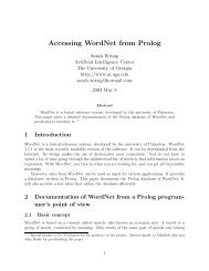
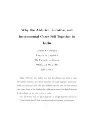
Three different forests are considered in this paper, namely a 40-stand northern forest [1]
(shown in Figure 1), the 73-stand Daniel Pickett Forest used in [1][2][7] (shown in Figure 2), and
a much larger 625-stand southern forest [1] (not shown). The relevant stand acreage, adjacency,
centroids, and time period harvest volumes are located under ―Northern US example forest,‖
―Western US example forest,‖ and ―Southern US example forest‖ at
http://www.warnell.forestry.uga.edu/Warnell/Bettinger/planning/index.htm. Three time periods
and a no-cut option are given for the problem. For the 40-stand forest the target harvest is
9,134.6 m 3 , for the 73-stand forest the target harvest is 34,467 MBF (thousand board feet), and
for the 625-stand forest the target harvest is 2,972,462 tons.
In summary, a harvest schedule is defined as an array of length equal to the number of
stands in the problem and whose elements are composed of integers on the range zero to three
inclusively, where 0 specifies the no-cut option, and 1 through 3 specify harvest periods. Thus,

7
solutions to the 40-, 73-, and 625-stand forest planning problems should be 40-, 73-, and 625-
length integer arrays. A valid schedule is a schedule with no adjacency violations, and an
optimal schedule is a valid schedule that minimizes f 1 .
Figure 1: 40-Stand Forest
Figure 2: 73-Stand Forest
Many algorithms have been applied towards this problem. In [1] Raindrop Optimization,
Threshold Accepting, and Tabu Search were used on the 40-, 73-, and 625-stand forest planning
problems. In [7], a Genetic Algorithm, integer Particle Swarm Optimization, Discrete Particle
Swarm Optimization, Raindrop Optimization, and Extremal Optimization were applied to the 73-
stand forest planning problem. In [2], a Priority Particle Swarm Optimization algorithm was
applied to the 73-stand forest problem.
In this paper, tests will be run with Raindrop Optimization and a new proposed algorithm,
Roulette Wheel Particle Swarm Optimization. Comparisons will be made between these test
results and the test results from [1], [2], and [7].

8
3 Raindrop Optimization
Described in [1], Raindrop Optimization (RO) is a stochastic point-based search
algorithm developed for the forest planning problem and was inspired by the ripples in a pond
generated from a falling raindrop. It starts with an initial valid schedule, perturbing the harvest
period at a random stand and repairing the resulting period adjacency violations in an everexpanding
ripple from the original perturbation, based on the centroids of the stands. The
perturbation repeats, and the best solution is reverted to after a certain interval. This perturbation
and repair process repeats until the termination criteria are met. The number of intervals until
reversion is called the reversion rate. Note that there is no set ratio between the number of
iterations and the number of fitness evaluations.
4 Particle Swarm Optimization
Particle swarm optimization (PSO) [3][4] is a stochastic population-based search
algorithm, where each member (called a particle) of the population (called a swarm) has a
dynamic velocity v and a location x, which is a point in the search space. The particle ―flies‖
through the search space using its velocity to update its location. The particle ―remembers‖ its
(local) best location p so far and is aware of the (global) best current location g for any particle in
the swarm. The attraction to the former is called the cognitive influence c 1 , and the attraction to
the latter is called the social influence c 2 . Each iteration of the PSO involves evaluating each
particle‘s location according to a fitness function, updating the local and global bests, updating
each particle‘s velocity, and updating each particle‘s location. The formula to update the velocity
and location of a particle in the i th dimension at time t is specified by the following:

9
where
is the inertia, r 1 and r 2 are all random numbers between 0 and 1, and t is the new
iteration step.
4.1 The Proposed PSO
In the proposed multi-valued algorithm Roulette Wheel PSO (RWPSO), a particle‘s
location in each dimension is generated by a roulette wheel process over that particle‘s roulette
wheel probabilities (here called its velocities) in that dimension; in a given dimension, the
particle has a velocity for every permissible location in that dimension. The algorithm
deterministically updates the velocity of each permissible location k in each dimension i for each
particle using the following formulas:
where
and m is the maximum step size, s is the social emphasis, and (1-s) is the cognitive emphasis.
The velocity v i,k is limited to the range [0,1], but is initially set to the reciprocal of the number of
permissible values in dimension i for two reasons: (1) the velocities represent roulette
probabilities and so together should sum to 1, and (2) with no domain knowledge of the
likelihood of each location k in the optimal solution, there is no reason to favor one location over
another. As previously mentioned, the particle‘s location in dimension i is determined by a
roulette wheel process, where the probability of choosing location k in dimension i is given by:
RWPSO parameters include the swarm size, the stopping criterion, the maximum step
size, and the social emphasis. The maximum step size controls the maximum rate at which the
RWPSO velocities will change and thus determines how sensitive the RWPSO is to the local and

10
global fitness bests. The social emphasis parameter determines what fraction of the maximum
step size is portioned to attraction to swarm global best versus how much is portioned to
attraction to the local best.
5 RWPSO Guide Functions
Since RWPSO will generate schedules that are not necessarily valid, the original
objective function f 1 cannot be used to guide the RWPSO, because f 1 does not penalize such
schedules. Thus, two fitness functions are derived that provide penalized values for invalid
schedules and also provide values for valid schedules which are identical to those produced by f 1 .
5.1 RWPSO Guide Function f 2
The fitness function f 2 is defined as:
where
and
where s is the harvest schedule, and s n is the scheduled harvest time of stand n.
Essentially, this function penalizes infeasible solutions by harvesting only those stands
that do not share a common scheduled harvest period with an adjacent stand; this is effectively a
temporary repair on the schedule to bring it into feasible space for fitness evaluation by omitting
all scheduled stand harvests that are part of an adjacency violation. As with f 1 , a n h n,k will be
either the volume from harvesting an entire stand n at time k or zero, if that stand is not
scheduled for harvest at time k.

11
5.2 Alternate RWPSO Guide Function f 3
The final fitness function f 3 uses a copy of the harvest schedule s, denoted s , and
modifies it throughout the fitness evaluation. It is the harmonic mean of f 2 and f 3 defined as:
where
Fitness function f 3 combines the strict penalizing fitness function f 2 with the more lenient
function f 3 . The function f 3 creates a copy of the schedule s and modifies this copy s during the
fitness evaluation. The function iteratively considers each stand in a schedule, and whenever an
adjacency violation is reached, the harvest volume of the currently considered stand is compared
to the total harvest sum of the adjacent stands having the same harvest period. If the former is
greater, then the stands adjacent to the current stand that violate the adjacency constraint are set
to no-cut in s . Otherwise, the current stand‘s harvest schedule is set to no-cut in s . As with f 1 ,
a n h n,k will be either the volume from harvesting an entire stand n at time k or zero, if that stand is
not scheduled for harvest at time k.
Note that for every feasible schedule, if the schedule is given to all three fitness
functions, each will yield identical fitness values, because the difference between them is in how

12
each one temporarily repairs an infeasible schedule in order to give it a fitness value; f 1 does no
repair, f 2 does a harsh repair, and f 3 combines f 2 with a milder repair f 3 .
6 Tests
Having a comparable measure of process time poses a problem in determining the
statistics of RO, because unlike RWPSO, the number of fitness evaluations is not the same as the
number of candidate solutions. In fact, RO may use many fitness evaluations in the process of
mitigating infeasibilities before offering a single candidate solution. Thus, two sets of statistics
will be offered for RO, where RO c specifies the case of limiting the number of candidate
solutions to 1,000,000, and RO f specifies the case of limiting to 1,000,000 the number of fitness
evaluations over 10 trials on the 40- and 73-stand forests. Each RWPSO parameter combination
was allowed to run for 10 trials of 1,000,000 fitness evaluations on the 40- and 73-stand forests.
In order to allow the algorithms more time on a more difficult problem, both algorithms were run
for 5 trials of 5,000,000 fitness evaluations on the 625-stand forest.
To find good parameter combinations, RO was run for 10 trials with reversion rates from
1 to 10 in steps of 1 on the 73-stand forest. RWPSO was run for 10 trials with f 2 on the 73-stand
forest with all combinations of the following parameters:
Swarm Size: {20, 40, 80, 160, 320, 640, 1280, 2560, 5120}
Max Step Size: {0.01, 0.05, 0.09, 0.13}
Social emphasis: {0.0, 0.25, 0.50, 0.75}
Even though RWPSO was tested over roughly 15 times the number of parameter
combinations of RO, run-time to complete all combinations was roughly the same between RO
and RWPSO. Note also that both algorithms were rather forgiving in terms of performance over
parameter combination variations. The best parameter combinations from this were used on the

13
remainder of the tests. Tests where RWPSO used f 2 are denoted RWPSO f2 . Similarly, tests
where RWPSO used f 3 are denoted RWPSO f3 .
One final variation on the configuration used for RWPSO is denoted RWPSO f3-pb . This
configuration involves biasing the initial velocities of the RWPSO using some expectation of the
likelihood of the no-cut option being included in the optimal schedule. It is expected that an
optimal schedule will have few no-cuts in its schedule. However, there is no expectation of the
other harvest period likelihoods. Therefore, the initial probabilities were tested for the following
cases:
7 Results
As with [1], the best reversion rate found for RO was 4 iterations. Similarly, the best
parameter combination found for RWPSO was swarm size 640, max step size 0.05, and a social
emphasis of 0.25. Of the initial no-cut probabilities tried, 0.04 gave the best objective values.
Table 3 shows the results of running each algorithm configuration on the 73-stand forest.
Clearly, the choice of how RO is limited—either by candidate solutions produced or by the
number of objective function evaluations—will substantially affect the solution quality. In fact,
if the number of objective function evaluations is considered as the termination criterion for both
algorithms, then every configuration of RWPSO outperforms RO on the 73-stand forest.
However, the use of f 3 improves the performance of RWPSO over RO, regardless of the
termination criterion used for RO. Also, note that although the use of biased initial no-cut
probability makes RWPSO f3-pb outperform RWPSO f3 , the largest gains by RWPSO in terms of

14
average objective values come from using f 3 instead of f 2 . Additionally, changing the function
that guides RWPSO drastically decreases the standard deviation of the solution quality.
Table 3: 73-Stand Forest Results
Best Solution Average Solution Standard Deviation
RO c 5,500,330 6,729,995 1,472,126
RO f 5,741,971 8,589,280 2,458,152
RWPSO f2 5,500,330 7,492,459 1,920,752
RWPSO f3 5,500,330 5,844,508 450,614
RWPSO f3-pb 5,500,330 5,786,583 437,916
The results for the 40-stand forest in Table 4 are similar to those in Table 3, except that
every configuration of RWPSO outperforms RO, regardless of the termination criterion used.
Additionally, RWPSO‘s greatest increase in performance came through using f 3 instead of f 2 .
Table 4: 40-Stand Forest Results
Best Solution Average Solution Standard Deviation
RO c 90,490 160,698 46,879
RO f 98,437 190,567 63,314
RWPSO f2 90,490 151,940 46,431
RWPSO f3 90,490 123,422 30,187
RWPSO f3-pb 90,490 113,624 23,475
The results from Table 5 illustrate that the 625-stand forest is much more difficult for
RWPSO than either of the other forests. RO with both termination criteria outperformed every
configuration of RWPSO. It can be noted that, just like for the other forests, the use of f 3
improved RWPSO‘s performance over f 2 , and the use of biased initial no-cut probability further
improved the quality of the RWPSO solutions.
Table 5: 625-Stand Forest Results
Best Solution Average Solution Standard Deviation
RO c 61,913,898,152 66,142,041,314 2,895,384,577
RO f 66,223,010,632 72,552,142,872 3,732,367,645
RWPSO f2 118,239,623,212 150,819,800,640 14,487,010,747
RWPSO f3 91,224,899,372 100,862,133,880 6,894,894,714
RWPSO f3-pb 87,444,889,432 95,872,673,094 6,808,823,161

15
8 Discussion
Some comparisons to the studies in Section 1 may be made, limited by the fact that they
limited the runtimes or iterations differently. Additionally, most of those studies deal only with
the 73-stand forest.
In [1], comparisons are difficult to make, because the number of fitness evaluations was
not recorded. In that paper, the best performance on the 73-stand forest was a best fitness of
5,556,343 and an average of 9,019,837 via RO. On the 40-stand forest, it was a best of 102,653
and an average of 217,470, and on the 625-stand forest via RO, it was a best of 69B and an
average of 78B via RO. In [7], the DPSO was allowed to run on the 73-stand forest up to 2,500
iterations with swarm sizes in excess of 1000, which translates to a maximum of 2.5M fitness
evaluations for a 1000 particle swarm. With DPSO, they obtained a best fitness in the range of
35M. In that paper, the best fitness value found was 5,500,391 via RO. In [2], the best
performance from their PPSO on the 73-stand forest was with 2,500 iterations of a size 500
swarm, which translates to 1,250,000 fitness evaluations. They achieved a best fitness of
5,500,330 and an average fitness of 8,831,332.
In comparison, the best results from this paper on the 73-stand forest are a best of
5,500,330 and an average of 5,786,583 after 1M fitness evaluations. RWPSO obtained the best
results of all the studies discussed for the 73-stand forest. Similarly, it outperformed on the 40-
stand forest with a best objective value of 90,490 and an average of 113,624. However, on the
625-stand forest, RO outperforms RWPSO, regardless of the termination criterion used.

16
9 Conclusion and Future Directions
The functions f 2 and f 3 promote Lamarckian learning by assigning fitnesses to infeasible
schedules based on nearby feasible schedules. The use of Lamarckian learning may be
beneficial in general on similar problems, and additional research would be required to test this.
RWPSO was formulated specifically for multi-valued nominal variable problems, and it
treats velocity more explicitly as a roulette probability than do other probability based PSOs.
Additionally, by expressing parameters of the algorithm in terms of their effects on the roulette
wheel, parameter selection is more intuitive. Future work needs to be done to determine if this
explicit roulette wheel formulation yields any benefit in general to RWPSO‘s performance over
other discrete PSOs.

17
References
[1] P. Bettinger, J. Zhu. (2006) A new heuristic for solving spatially constrained forest
planning problems based on mitigation of infeasibilities radiating outward from a forced
choice. Silva Fennica. Vol. 40(2): p315-33.
[2] P. W. Brooks, and W. D. Potter. (2011) ―Forest Planning Using Particle Swarm
Optimization with a Priority Representation‖, in Modern Approaches in Applied
Intelligence, edited by Kishan Mehrotra, Springer, Lecture Notes in Computer Science.
Vol. 6704: p312-8.
[3] R. Eberhart, and J. Kennedy. (1995) A new optimizer using particle swarm theory.
Proceedings 6th International Symposium Micro Machine and Human Science, Nagoya,
Japan. p39-43.
[4] J. Kennedy, and R. Eberhart. (1995) Particle Swarm Optimization. Proceedings IEEE
International Conference Neural Network, Perth, WA, Australia. Vol. 4: p1942-8.
[5] J. Kennedy, and R. Eberhart. (1997) A Discrete Binary Version of the Particle Swarm
Algorithm. IEEE Conference on Systems, Man, and Cybernetics, Orlando, FL. Vol. 5:
p4104-9.
[6] J.H. Holland. (1975) Adaptation in Natural and Artificial Systems. Ann Arbor, MI: The
University of Michigan Press.
[7] W.D. Potter, E. Drucker, P. Bettinger, F. Maier, D. Luper, M. Martin, M. Watkinson, G.
Handy, and C. Hayes. (2009) ―Diagnosis, Configuration, Planning, and Pathfinding:
Experiments in Nature-Inspired Optimization‖, in Natural Intelligence for Scheduling,
Planning and Packing Problems, edited by Raymond Chong, Springer-Verlag,Studies in
Computational Intelligence. Vol. 250: p267-94.

18
Chapter 3
Probability Update Analysis for Probability-Based
Discrete Particle Swarm Optimization Algorithms 2
2 Jared Smythe, Walter D. Potter, and Pete Bettinger. Submitted to Applied Intelligence: The
International Journal of Artificial Intelligence, Neural Networks, and Complex Problem-Solving
Technologies, 04/03/2012.

19
Abstract: Discrete Particle Swarm Optimization algorithms have been applied to a variety of
problems with nominal variables. These algorithms explicitly or implicitly make use of a
roulette wheel process to generate values for these variables. The core of each algorithm is then
interpreted as a roulette probability update process that it uses to guide the roulette wheel
process. A set of intuitive requirements concerning this update process is offered, and tests are
formulated and used to determine how well each algorithm meets the roulette probability update
requirements. Roulette Wheel Particle Swarm Optimization (RWPSO) outperforms the others in
all of the tests.
1 Introduction
Some combinatorial optimization problems have discrete variables that are nominal,
meaning that there is no explicit ordering to the values that a variable may take. To illustrate the
difference between ordinal and nominal discrete variables, consider the discrete ordinal variable
where x represents the number of transport vehicles required for a given
shipment. There is an order to these numbers such that some values of x may be ―too small‖ and
some values may be ―too large‖. Additionally, the ordering defines a ―between‖ relation, such
that 3 is ―between‖ 2 and 4. In contrast, consider the discrete variable
, where
is an encoding of the nominal values {up, down, left, right, forward, background}.
Clearly, no values of y may be considered ―too small‖ or ―too large‖, and no value of y is
―between‖ two other values.
Discrete Particle Swarm algorithms exist that have been applied to problems with
nominal variables. Shortly after the creation of Particle Swarm Optimization (PSO) [2][3], a
binary Discrete PSO was formulated [4] and used on nominal variable problems by transforming
the problem variables into binary, such that a variable with 8 permissible values becomes 3

20
binary variables. In [5] and [8], the continuous PSO‘s locations were limited and rounded to a
set of integers, although this still yields a discrete ordinal search. In [1] and [6], a discrete multivalued
PSO was formulated for job shop scheduling. In [7] a different discrete multi-valued
PSO was developed by Pugh.
Except for in [5] and [8], an approach common to all the algorithms is a process where
for each location variable in each particle, the PSO: (1) generates a set of n real numbers having
some correspondence to the probabilities of the n permissible values of that variable and (2)
applies a roulette wheel process on those probabilities to choose one of those permissible values
as the value of that variable. Because this process chooses the value for a single variable in a
particle in the swarm, it differs from the roulette wheel selection used by some algorithms to pick
parents for procreation. The roulette probabilities are determined by:
where y is the variable, k is a possible value of y, z k is the number generated by the PSO to
express some degree of likelihood of choosing k, and n is the number of permissible values for y.
In [4], this process is not explicitly presented, but the final step in the algorithm may be
interpreted this way—this will be covered in more detail. The algorithms differ in how they
generate each z k , and thus the manner in which they update the roulette probabilities differs in
arguably important ways that may affect their general performance.
This paper presents some roulette probability update requirements that PSOs should
intuitively satisfy in order to perform well in general on discrete nominal variable problems. The
behavior of each of these discrete PSOs is explored through problem-independent tests
formulated around the roulette probability update requirements.

21
2 Motivations and Metrics
Some intuitive requirements about the roulette probability updates can be assumed a
priori. These requirements will be used to measure the relative quality of each PSO‘s probability
update performance. These requirements are that changes to roulette probabilities should be:
(a) Unbiased (symmetric) with respect to encoding. By this it is meant that the updates
should not behave differently if the nominal variables are encoded in a set of integers
differently. This requirement essentially ensures that the un-ordered nature of the
variables is preserved, regardless of the encoding.
(b) Based on the PSO‘s knowledge. The only knowledge a PSO has at any given
moment is its current location and the locations of the global and local bests. It
should not act on ignorance. Thus, it should not alter the roulette probability for a
value that is not the current location, the global best, or the local best. Otherwise,
false positives and false negatives may mislead the PSO.
(c) Intuitively related to the PSO parameters. The parameters should have intuitive and
linear effects on the probability updates. This requirement makes finding good
parameter sets faster and more efficient, as well as making it easier to fine tune the
parameters.
Requirement (a) is important because it ensures that the encoding of the variable values
treats all the encoded values equally. Otherwise, the PSO will tend towards variable values
based on artifacts of the encoding and not based on their fitness. For example, if a variable‘s
values {L,R,U,D} (Left, Right, Up, Down) were encoded in the problem space as {0,1,2,3} with
a certain PSO tending towards 0 (the encoding of ‗L‘), and when encoded as {1,2,0,3}, the PSO
still tended towards 0 (now the encoding of ‗U‘), then the PSO behavior differs solely because

22
{L,R,U,D} was encoded differently. Thus, (a) is really the requirement that the encoding should
be transparent to the PSO. This also means that the PSO should be unbiased with respect to
different instances of the same configuration—this will be discussed in more detail.
Another way to phrase (b) is that PSOs should tend to update along gradients determined
by the PSO‘s knowledge; since the values of the variable are nominal and thus orthogonal, if the
PSO does not have any knowledge of a value (e.g. the value is not a global or local best and is
not the current location 3 ), no gradient is evident. For instance, consider the values {L,R,U,D}, if
‗L‘ is both the global and local best value, and ‗U‘ is the current value, then it is known that ‗L‘
has higher fitness than ‗U‘, and thus there is a gradient between them with increasing fitness
towards ‗L‘. Note that this PSO wouldn‘t have any knowledge about how the fitnesses of ‗R‘
and ‗D‘ compare with ‗L‘ or ‗U‘, and thus no gradient involving ‗R‘ or ‗D‘ is evident. Thus, the
PSO should not update the probabilities of ‗R‘ and ‗D‘. Also, note in general that altering
roulette probabilities without knowing if they are part of good or bad solutions may lead to false
positives (a high probability for an unknown permissible value) or false negatives (a low
probability for a known permissible value) that may severely hamper exploitation and
exploration, respectively, because this effect is independent of the fitness values related to them.
Requirement (c) ensures that parameter values have a linear relationship with algorithm
behavior, which yields more intuitive parameter search. For instance, for a given parameter a
value of 0.25 intuitively (and generally naively) should result in behavior exactly halfway
between the behavior of having value 0 and the behavior of having value 0.5. This is helpful
because generally the novice PSO user will tend to experiment with parameter values in a linear
manner—i.e. balancing opposing parameters with a ratio of 0, then 0.25, then 0.5, then 0.75, and
3
Such permissible values that are not the global best, local best, or current location will be
termed unknown, because they are not part of the PSO‘s knowledge.

23
then 1.0, because it is assumed that the parameter values have a linear relationship with the
algorithm behaviors.
Lacking any domain knowledge or prior tests, the manner in which the roulette
probabilities are updated may provide insight about the PSO‘s search behavior. This knowledge
can be obtained in a problem-independent manner by studying how the probabilities are updated
in a single dimension given a current location, local best, and global best for that dimension.
3 Particle Swarm Optimization
Particle swarm optimization (PSO) [2][3] is a stochastic population-based search
algorithm, where each member (called a particle) of the population (called a swarm) has a
dynamic velocity v and a location x, which is a point in the search space. The particle ―flies‖
through the search space using its velocity to update its location. The particle ―remembers‖ its
(local) best location p so far and is aware of the (global) best current location g for any particle in
the swarm. The attraction to the former is called the cognitive influence c 1 , and the attraction to
the latter is called the social influence c 2 . Every iteration of the PSO involves evaluating each
particle‘s location according to a fitness function, updating the local and global bests, updating
each particle‘s velocity, and updating each particle‘s location. The formula to update the velocity
and location of a particle in the i th dimension at time t is specified by the following:
where
is the inertia, r 1 and r 2 are random numbers between 0 and 1, and t is the new iteration
step.

24
3.1 Binary Discrete PSO
An early discrete PSO variant DPSO allows for a real valued velocity but uses a binary
location representation [4]. The velocity and location updates for the i th bit of a particle in a
DPSO are computed as follows:
where r 1 , r 2 , and r 3 are random numbers between 0 and 1. The update for x i can be interpreted as
a roulette wheel process where:
where
and
In cases where the nominal variable x is split into two binary variables x’ i,0 and x’ i,1 with
velocities v’ i,0 and v’ i,1 , the roulette wheel process becomes:
where
, , and
This process can be extended to more than two binary variables, if necessary, by a similar
process.
3.2 Chen’s PSO
This PSO [1], which we will call CPSO, builds upon the original binary DPSO described
by [4] and a multi-valued PSO scheme described in [6]. Its original use was in flow-shop

25
scheduling. It uses a continuous PSO dimension for every discrete value of a single dimension
in the problem space. Thus, the PSO space is a
vector of real numbers, where s is the
number of dimensions in the problem space and t is the number of permissible values in each
dimension. It updates the velocity somewhat differently than do the previous discrete PSOs, but
like the binary DPSO it takes the sigmoid of the velocities and uses a roulette wheel process to
determine the roulette probabilities.
First, a function to convert from the discrete location to a binary number for each
permissible location, indicating if the PSO is at that permissible value or not, must be defined
using the following:
Accordingly, the velocity of permissible location k in dimension i is updated using the following
functions:
where
The roulette probabilities are then generated from the sigmoid of the velocities by a roulette
wheel process. The roulette probabilities are generated by:
Here the purpose of the sigmoid is not to generate probabilities from the velocities as
with DPSO; instead, the roulette wheel process explicitly performs this function.

26
3.3 Pugh’s MVPSO
Like CPSO, this algorithm described in [7] uses a continuous PSO dimension for every
permissible value of every dimension in the problem space. Thus, the PSO‘s space is a
vector of real numbers, where s is the number of problem space dimensions and t is the number
of permissible values in each dimension. As with CPSO, MVPSO uses the standard continuous
PSO update rules, but during the fitness evaluation phase, it takes the sigmoid of the n locations
and uses those values to generate the schedule by a roulette wheel scheme. Thus, the following
are the update functions:
where c is chosen each iteration such that
. Pugh calls c the value that
―centers‖ the particles. Unfortunately, the value c cannot be found analytically, so it must be
found by numerical approximation.
3.4 RWPSO
Described in [9], Roulette Wheel PSO (RWPSO) is a multi-valued PSO with an explicit
relation to a roulette wheel. In RWPSO, a particle‘s location in each dimension is generated by a
roulette wheel process over that particle‘s velocities (often the same as its roulette wheel
probabilities) in that dimension; in a given dimension, the particle has a velocity for every
permissible location in that dimension. The algorithm deterministically updates the velocity of
each permissible location k in each dimension i for each particle using the following formulas:

27
where
and m is the maximum step size, s is the social emphasis, and (1-s) is the cognitive emphasis.
The velocity v i,k is limited to the range [0,1], but is initially set to the reciprocal of the number of
permissible values in dimension i for two reasons: (1) the velocities closely represent roulette
probabilities and so together should sum to 1, and (2) with no domain knowledge of the
likelihood of each location k in the optimal solution, there is no reason to favor one location over
another. As previously mentioned, the particle‘s location in dimension i is determined by a
roulette wheel process, where the probability of choosing location k in dimension i is given by:
Note that unless the sum of the velocities deviates from 1, .
RWPSO parameters include the swarm size, the stopping criterion, the maximum step
size, and the social emphasis. The maximum step size controls the maximum rate at which the
RWPSO velocities will change and thus determines how sensitive the RWPSO is to the local and
global fitness bests. The social emphasis parameter determines what fraction of the maximum
step size is portioned to attraction to the swarm global best versus how much is portioned to
attraction to the local best.
4 Tests
For simplicity, the problem space will be chosen as having a single dimension.
Additionally, since PSO knowledge only contains information about the locations of the local
best, the global best, and the current position, four permissible values will be chosen. This is the
smallest space that allows for the local best, global best, current position, and unknown position

28
to be at different locations in the search space without any overlap. The permissible values are
encoded as {0, 1, 2, 3}.
Unless otherwise stated, the algorithm settings are as follows:
Algorithm Parameter Settings
DPSO cognitive influence: 1
social influence: 3
inertia: 1.2
Vmax: 4
MVPSO cognitive influence: 1
social influence: 3
inertia: 1.2
Vmax: 4
CPSO cognitive influence: 1
social influence: 3
inertia: 1.2
Vmax: 4
RWPSO Max step size: 0.05
Social emphasis: 0.25
Table 1: The algorithm parameter settings
The following sections experiment with multiple discrete PSOs under various
circumstances in the aforementioned test space to study how each PSO updates its roulette
probabilities. Based on the results and how they relate to requirements (a)-(c), certain
conclusions about PSO performance can be made.
4.1 Single Iteration Probability Updates
The purpose of this test is to analyze the average roulette probability update behavior of
the PSO by examining the probabilities before and after the PSO updates looking for violations
of requirements (a) and (b). Here, violations of (a) will only appear as inconsistencies in the
updates of unknown values‘ probabilities since they should be treated identically. Violations of
(b) will appear as changes in the average probabilities of the unknown values.

29
There are only five possible configurations of the relative locations of the current
location, the global best, and the local best with respect to each other in a non-ordered space.
They are:
(1) The global best, local best, and current locations are the same.
(2) The global best and current locations are the same, but the local best location is
different.
(3) The local best and current locations are the same, but the global best location is
different.
(4) The local best and global best locations are the same, but the current location is
different.
(5) The local best, global best, and current locations are all different.
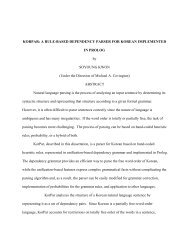
Figure 10 shows ideal average probability updates expected for this test corresponding to
each of these configurations, where the size of the slice on the roulette wheel represents the
roulette probability. It is ideal because the unknown values‘ probabilities are treated identically,
satisfying (a), and those same probabilities remain unchanged after the update, satisfying (b).
Figure 1: The ideal probability updates
Because we assume that restriction (a) must hold, we can choose a particular encoding
(or instance) for each configuration without loss of generality. For our tests, where the

30
permissible values have been assumed to be from the set {0, 1, 2, 3}, the test instance of each
configuration is as follows:
Configuration
Instance
Current Global best Local best
1 0 0 0
2 0 0 1
3 0 1 0
4 0 1 1
5 0 1 2
Table 2: The permissible values at the current, local best, and global best locations
Thus, the instances in Table 2 would encode the roulette wheel in Figure 1 thusly: the upper left
quadrant as 0, the upper right quadrant as 1, the lower left quadrant as 2, and the lower right
quadrant as 3.
In order to simulate the behavior of the PSO for any iteration during its run, the
probabilities or velocities were randomized before performing this test. The test consists of the
following steps:
1) Initialize the algorithm, setting the current value, the global best, and the local best
appropriate to the instance being considered and randomizing the velocities.
2) Let the PSO update the velocities and probabilities.
3) Let the PSO generate the new current location.
4) Record the new current location.
5) Repeat steps 1-4 for 100,000,000 trials.
6) Determine the portion of the trials that generated each location.
7) Repeat steps 1-6 for the five instances.
Because the PSOs are set to have random probabilities initially, the probability of generating
each location is 25% before the update is applied. This was verified by 100,000,000 trials of
having the PSOs generate a new current location without having updated the probabilities.

31
The results are shown in Table 3, where P(x) is the portion of the trials for which the
current location generated was x.

Configuration 1 Configuration 2 Configuration 3 Configuration 4 Configuration 5
Name P(0) P(1) P(2) P(3) P(0) P(1) P(2) P(3) P(0) P(1) P(2) P(3) P(0) P(1) P(2) P(3) P(0) P(1) P(2) P(3)
DPSO 25% 25% 25% 25% 21% 29% 21% 29% 15% 35% 15% 35% 12% 38% 12% 38% 12% 30% 17% 41%
MVPSO 25% 25% 25% 25% 17% 35% 24% 24% 7% 52% 21% 21% 4% 59% 18% 18% 4% 49% 27% 19%
CPSO 25% 25% 25% 25% 20% 29% 25% 25% 13% 35% 26% 26% 9% 37% 27% 27% 9% 35% 30% 26%
RWPSO 25% 25% 25% 25% 21% 29% 25% 25% 24% 26% 25% 25% 20% 30% 25% 25% 20% 26% 29% 25%
Table 3: The resulting roulette probabilities after each algorithm’s update
32

33
In Table 3, the shaded regions correspond to locations for which the PSO has no
knowledge—in other words, the location is not the current location, the local best, or the global
best. Thus, DPSO violates requirement (a) in configurations 2, 3, and 4 by not treating the
shaded regions identically. Because of requirement (b), these shaded roulette probabilities
should not on average be altered from 25% by the PSO. Both DPSO and MVPSO violate (b) by
altering these probabilities in configurations 2, 3, 4, and 5, and CPSO violates (b) in
configurations 3, 4, and 5, although by not as much. The only PSO which does not violate (a) or
(b) here is RWPSO.
4.2 Probability Update Convergence Behavior
The purpose of this test is to analyze the long term behavior of the PSO, if the local best
and global best are set at different locations and the balance between the social and cognitive
parameters is set differently per run, specifically to test for violations of requirements (c). This
test can also inform us how well the PSO mixes components from the local and global bests to
form the new current location, as well as how linearly the PSO parameters affect the mixing
process. Additionally, the analysis can also show how consistently the PSO mixes these
components. Violations of (c) will appear as nonlinear effects resulting from varying algorithm
parameters linearly.
In order to make these observations, we need a single parameter for all the algorithms in
the range [0,1] that determines the mixing of the social and cognitive influence parameters. For
RWPSO, the parameter s fulfills this need. However, for the other algorithms, we must construct
a parameter to parameterize the social and cognitive influences of the algorithms. A
parameterization is created for the other algorithms using:

34
where s is the social emphasis, i.e. the fraction of attraction directed towards the global best.
Using the conventional wisdom that the social and cognitive influences sum to 4, this is
rearranged so that we get the social and cognitive influences thusly:
and
Using this parameterization, we now can test how setting the balance between the social
attraction and cognitive attraction parameters in each algorithm affects the roulette probability
updates.
This test follows the following steps:
1) Set the current location randomly, set 0 as the global best, and set 1 as the local best.
2) Initialize the particle to its starting state, as defined by each algorithm.
3) Update the PSO velocities or probabilities to generate the new current location.
4) Repeat step 3 for 1000 iterations.
5) Record the last iteration‘s encoded probability for choosing each of the four locations.
6) Repeat steps 1-5 for 100,000 trials.
7) Compute the average of each location‘s probability generated at the end of each trial,
and compute the standard deviation of the probability for the first location.
8) Repeat steps 1-7 for each value of s.
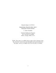
The reader might assume some balance in attraction to the global best and local best
corresponding to the balance between the social and cognitive influences (determined by s).
However, Figure 2 shows how RWPSO is the only algorithm whose social emphasis parameter s
acts linearly on the probability of choosing the global best location, indicating that the balance in
attraction to the global best and local best corresponds linearly to the balance parameter

Average Probability of Location 0
35
established by s. Thus, it satisfies requirement (c), whereas the others do not, because the
relationship between s and the balance between the global best and local best is linear.
1
0.9
0.8
0.7
0.6
0.5
0.4
0.3
0.2
0.1
0
0 0.1 0.2 0.3 0.4 0.5 0.6 0.7 0.8 0.9 1
s
RWPSO
DPSO
MVPSO
ChenPSO
Figure 2: The effect of s on the average probability of location 0
Figure 3 shows the standard deviation of the roulette probability of choosing the global
best given various values of s. Again, RWPSO comes out as having the most consistent behavior
over the parameter s. This shows that the mixing of the global best and local best is not
consistent for the other algorithms when the mix is supposed to be nearly evenly distributed
(s=0.5). More importantly, the s does not have a linear relationship with the standard deviation
of the probability of choosing the global best permissible value. Thus, this is a violation of the
parameter linearity requirement (c) for all the algorithms, although RWPSO has the flattest curve
closest to being linear.

Sum of average probabilities for nonbest
locations
Standard deviation of the probability of
Location 0
36
0.35
0.3
0.25
0.2
0.15
0.1
0.05
RWPSO
DPSO
MVPSO
ChenPSO
0
0 0.1 0.2 0.3 0.4 0.5 0.6 0.7 0.8 0.9 1
s (for RWPSO) or c1/(c1+c2)
Figure 3: The effect of s on the standard deviation of the probability of location 0
Figure 4 shows the sum of probabilities of the non-best locations. Only DPSO and
RWPSO have a linear effect on this sum and thus satisfy the parameter linearity requirement (c).
Additionally, MVPSO and CPSO violate (b)—which requires that updates only affect current
values and best values—because the only way such high sums could be generated is if the PSO
increased the probability of the non-bests without having them as a current location, because
current location probabilities do not increase on average for those PSOs, as shown in Table 3.
0.45
0.4
0.35
0.3
0.25
0.2
0.15
0.1
0.05
0
0 0.1 0.2 0.3 0.4 0.5 0.6 0.7 0.8 0.9 1
s (for RWPSO) or c1/(c1+c2)
RWPSO
DPSO
MVPSO
ChenPSO
Figure 4: The effect of s on the sum of the average probabilities of the non-best values

37
4.3 Discussion
In Table 3, on average Pugh‘s MVPSO penalizes every permissible value where
knowledge is lacking (where the permissible value was not the local best location, global best
location, or current location). This inhibits exploration because if the unknown values‘ roulette
probabilities are decreased, then those permissible values are less likely to be chosen in the
location update. This means they will likely continue to be in the unknown, which means that
MVPSO will continue to decrease their probabilities. However, this is inconsistent because it
does not occur in configuration 1. As discussed when introducing requirement (a), there is no
gradient justification for this.
The behavior of DPSO in Table 3 is not unexpected due to the way that the roulette
probabilities are generated from the binary encoding of the four permissible values. Consider
Figure 5, where social influence has been set higher than cognitive influence and where x, l, and
g are the current location, local best location, and global best location, respectively. It shows two
different update cases where the roulette probability of the current location has been penalized.
Case 1 is an update resulting in an increase in the roulette probability of the unknown
permissible value and Case 2 is an update resulting in a smaller roulette probability of the
unknown permissible value. This is an artifact of the encoding of the four permissible values
into two binary DPSO location variables. 4
4 An additional artifact of the encoding is that for permissible values A and B encoded as binary
strings a and b with Hamming distance , it is not possible that both and
, violating requirement (a).

38
Figure 5: Probability update for DPSO
This is additional evidence that DPSO violates requirement (a), because in the two different
instances of configuration (5) it updates the roulette probabilities of the unknown permissible
values differently.
CPSO updates in Table 3 increased some of the roulette probabilities of the permissible
values where knowledge was lacking; however, these increases were by a very small amount and
thus were a small violation of requirement (b). RWPSO did not modify the roulette probabilities
of those values at all.
In Figure 2, DPSO and MVPSO showed an almost sigmoidal relationship between the
cognitive-social balance and the average updated probability of the global best position. CPSO
exhibited a much more bizarre curve. The most important thing to note about the effect of their
curves is that parameter testing DPSO, MVPSO, and CPSO will be much less intuitive since
varying s only seems to noticeably effect the roulette probabilities when s varies on the range 0.3
to 0.7, which translates to typical c 1 and c 2 values in the range 1.2 to 2.8. This also explains the
popularity of choosing social and cognitive influence parameter values close to 2. In contrast,
RWPSO exhibits a linear relationship between s and the roulette probability of the global best
permissible value. This means that changes to s exhibit predictable changes to the roulette
probability of the global best permissible value.
On the small s range of 0.3 to 0.7, there is also a large standard deviation of the average
roulette probabilities for DPSO, MVPSO, and CPSO shown in Figure 2. This means that in use,

39
the probabilities themselves may be more random and thus less capable of directing the search.
The RWPSO standard deviation curve over s is both more evenly distributed and lower,
indicating more consistency and greater ability to direct the search.
As shown in Figure 4, both MVPSO and CPSO have a tendency to retain high
probabilities for non-best locations even after 1,000 iterations. This may inhibit exploitation of
good results, since the PSOs are forced to continue incorporating permissible values that are not
part of known good solutions, with a rather high probability. In other words, on average, with a
typical s value of 0.5 (where c 1 =c 2 =2) almost 40% of the problem space variables will be at
neither the local nor global best even after 1,000 iterations when using CPSO. Similarly, when s
is on the range 0.3 to 0.7, over 12.5% of the problem space variables will be at neither the local
nor global best even after 1,000 iterations when using MVPSO. Additionally, this effect is not
linear and thus not predictable when varying the parameter values.
Of the PSOs considered, the RWPSO violated requirements (a)-(c) the least. Although
the constraints were intuitive and determined a priori, violating (a)-(c) will put a PSO at a
distinct disadvantage at being a general-purpose algorithm for nominal variable problems.
4.4 Conclusion and Future Work
The goal of this paper was to discuss general requirements for a general-purpose multivalue
PSO for problems with nominal variables and to observe the performance of four PSO
algorithms on problem-independent tests with respect to satisfying those general requirements.
The results showed that DPSO‘s performance depends on how its permissible values are
encoded per problem, because it violated requirement (a). The results also showed that DPSO,
MVPSO, and CPSO all inconsistently applied the heuristic of updating probabilities according to
gradients, because they violated requirement (b). Finally, the results showed that because DPSO,

40
MVPSO, and CPSO all have nonlinear parameter effects (violating (c)), algorithm behavior is
unpredictable and counterintuitive with respect to parameter values, which has led to a
―conventional wisdom‖ of choosing cognitive and social values close to 2 without understanding
why this is desirable, regardless of the fitness landscape of the problem.
In contrast, RWPSO satisfies (a) and so is not sensitive to the manner of encoding, and
thus no prior domain knowledge is necessary to optimize the encoding of the problem variables‘
permissible values. Secondly, RWPSO satisfies (b) and so consistently applies the heuristic of
updating the probabilities along the known fitness gradients, which keeps the algorithm from
working against itself. Finally, RWPSO satisfies (c) by having linear parameter effects with no
―sweet spot‖, allowing parameter variations to have exactly the effect intuitively ascribed to
them—a weighted sum of two parameter‘s values yields a similarly weighted sum of their
probability update behaviors.
Additional work is necessary to empirically verify the performance predictions
concerning these algorithms on various problems with nominal variables. These tests will have
to be varied and large in number in order to test general performance. Further tests also need to
be formulated to test the effect of the magnitude of the roulette probability updates on the
convergence behavior of each algorithm.

41
References
[1] R. Chen. (2011) ―Application of Discrete Particle Swarm Optimization for Grid Task
Scheduling Problem‖, in Advances in Grid Computing, edited by Zoran Constantinescu,
Intech. pp. 3-18.
[2] R. Eberhart and J. Kennedy. (1995) A New Optimizer Using Particle Swarm Theory.
Proceedings 6th International Symposium Micro Machine and Human Science, Nagoya,
Japan. pp. 39-43.
[3] J. Kennedy and R. Eberhart. (1995) Particle Swarm Optimization. Proceedings IEEE
International Conference Neural Network, Perth, WA, Australia. 4: 1942-1948.
[4] J. Kennedy and R. Eberhart. (1997) A Discrete Binary Version of the Particle Swarm
Algorithm. IEEE Conference on Systems, Man, and Cybernetics, Orlando, FL. 5: 4104-
4109.
[5] E. C. Laskari, K. E. Parsopoulos, and M. N. Vrahatis. (2002) Particle Swarm
Optimization for Integer Programming. Proceedings IEEE Congress on Evolutionary
Computation, CEC‘02, Honolulu, HI, USA. pp. 1582–1587.
[6] C. J Liao, C.T. Tseng, and P. Luarn. (2007) A Discrete Version of Particle Swarm
Optimization for Flowshop Scheduling Problems. Computers and Operations Research.
34(10): 3099-111.
[7] J. Pugh and A. Martinoli. (2005) Discrete Multi-Valued Particle Swarm Optimization.
Proceedings IEEE Swarm Intelligence Symposium, SIS 2005. pp. 92-99.
[8] A. Salman, I. Ahmad, and S. Al-Madani. (2002) Particle Swarm Optimization for Task
Assignment Problem. Microprocessors and Microsystems. 26(8): 363–371.
[9] J. Smythe, W. D. Potter, and P. Bettinger (under review) Application of a New Multi-
Valued Particle Swarm Optimization to Forest Harvest Schedule Optimization, submitted
Feb 2012.

42
Chapter 4
Summary and Conclusion
In Chapter 2 RWPSO and Raindrop Optimization were applied to three forest planning
problems. It was shown that RWPSO strongly outperformed every other published result using a
PSO variant. Furthermore, RWPSO outperformed every other algorithm discussed on each of the
three forest planning problems, except for Raindrop Optimization, which produced superior
results on the 625-stand forest. Further research will determine how other algorithms fare on the
625-stand problem, as well.
In Chapter 3 the goal was to propose general constraints for probability-based PSOs for
nominal variable problems. These constraints require consistency of performance across nominal
value encodings, probability updates only according to PSO knowledge, and linear update
changes in relation to parameter variation. It is argued that a probability-based PSO must satisfy
these constraints in order to be a more effective general-purpose solver for nominal variable
problems. Finally, four PSO variants are tests with experiments formulated to assess satisfaction
of the three constraints, and RWPSO is found to violate them the least. This is claimed to have
important ramifications on its general behavior. Firstly, the order of encoding of the nominal
variables is inconsequential. Secondly, the heuristic of updating probabilities with respect only to
the PSOs knowledge is maintained. Finally, obtaining good parameters is easier, especially for
novice users, because update changes correspond linearly to parameter changes.

43
References
P. Bettinger, J. Zhu. (2006) A new heuristic for solving spatially constrained forest planning
problems based on mitigation of infeasibilities radiating outward from a forced choice.
Silva Fennica. Vol. 40(2): p315-33.
P. W. Brooks, and W. D. Potter. (2011) ―Forest Planning Using Particle Swarm Optimization
with a Priority Representation‖, in Modern Approaches in Applied Intelligence, edited by
Kishan Mehrotra, Springer, Lecture Notes in Computer Science. Vol. 6704: p312-8.
R. Chen. (2011) ―Application of Discrete Particle Swarm Optimization for Grid Task Scheduling
Problem‖, in Advances in Grid Computing, edited by Zoran Constantinescu, Intech. pp.
3-18.
R. Eberhart and J. Kennedy. (1995) A New Optimizer Using Particle Swarm Theory.
Proceedings 6th International Symposium Micro Machine and Human Science, Nagoya,
Japan. pp. 39-43.
J.H. Holland. (1975) Adaptation in Natural and Artificial Systems. Ann Arbor, MI: The
University of Michigan Press.
J. Kennedy and R. Eberhart. (1995) Particle Swarm Optimization. Proceedings IEEE
International Conference Neural Network, Perth, WA, Australia. 4: 1942-1948.
J. Kennedy and R. Eberhart. (1997) A Discrete Binary Version of the Particle Swarm Algorithm.
IEEE Conference on Systems, Man, and Cybernetics, Orlando, FL. 5: 4104-4109.
E. C. Laskari, K. E. Parsopoulos, and M. N. Vrahatis. (2002) Particle Swarm Optimization for
Integer Programming. Proceedings IEEE Congress on Evolutionary Computation,
CEC‘02, Honolulu, HI, USA. pp. 1582–1587.
C. J Liao, C.T. Tseng, and P. Luarn. (2007) A Discrete Version of Particle Swarm Optimization
for Flowshop Scheduling Problems. Computers and Operations Research. 34(10): 3099-
111.
W.D. Potter, E. Drucker, P. Bettinger, F. Maier, D. Luper, M. Martin, M. Watkinson, G. Handy,
and C. Hayes. (2009) ―Diagnosis, Configuration, Planning, and Pathfinding:
Experiments in Nature-Inspired Optimization‖, in Natural Intelligence for Scheduling,
Planning and Packing Problems, edited by Raymond Chong, Springer-Verlag,Studies in
Computational Intelligence. Vol. 250: p267-94.
J. Pugh and A. Martinoli. (2005) Discrete Multi-Valued Particle Swarm Optimization.
Proceedings IEEE Swarm Intelligence Symposium, SIS 2005. pp. 92-99.

A. Salman, I. Ahmad, and S. Al-Madani. (2002) Particle Swarm Optimization for Task
Assignment Problem. Microprocessors and Microsystems. 26(8): 363–371.
44