An Evaluation of Feature Extraction Methods for Vehicle ... - ECS

An Evaluation of Feature Extraction Methods for Vehicle
Classification Based On Acoustic Signals
Ahmad Aljaafreh, Student Member, IEEE and Liang Dong, Senior Member, IEEE
Abstract— Classification of ground vehicles based on acoustic
signals can be employed effectively in battlefield surveillance,
traffic control, and many other applications. The classification
performance depends on the selection of signal features that
determine the separation of different signal classes. In this paper,
we investigate two feature extraction methods for acoustic
signals from moving ground vehicles. The first one is based on
spectrum distribution and the second one on wavelet packet
transform. These two methods are evaluated using metrics
such as separability ratio and the correct classification rate.
The correct classification rate not only depends on the feature
extraction method but also on the type of the classifier. This
drives us to evaluate the performance of different classifiers,
such K-nearest neighbor algorithm (KNN), and support vector
machine (SVM). It is found that, for vehicle sound data, a
discrete spectrum based feature extraction method outperforms
wavelet packet transform method. Experimental results verify
that support vector machine is an efficient classifier for vehicles
using acoustic signals.
I. INTRODUCTION
DUE to the rapid progress in communications and sensor
technologies, wireless sensor networks become very
attractive area of research . It has been implemented in many
disciplines and fields. There are uncountable applications for
wireless sensor network. Data aggregation, event detection,
monitoring, and tracking are some of the main applications
for wireless sensor networks. Some of these applications
deals with continuous signals, like sounds, images, videos,
vibrations, magnetic field. Such applications need signal
processing. Signal processing in wireless sensor network is
mainly divided into the following categories: detection, classification,
localization, and tracking. In this research we will
investigate vehicle classification in wireless sensor network
using acoustic signals. Moving ground vehicles affect the
environment in different ways. Vehicle emits heats, sounds,
magnetic field. There are many approaches that investigated
vehicle identification based on different kinds of signals.
The most promising approach for vehicle identification is
the one that is based on acoustic signals. Moving vehicles
emit characteristic sounds. These sounds are generated
from moving parts, frictions, winds, emissions, tires,...etc.
Assuming that similar vehicles that have the same working
conditions generate the same sounds then these sounds can be
used to classify vehicles [1]. This motivates people to study
This work was supported in part by the DENSO North America Foundation
and by the Faculty Research and Creative Activities Award of Western
Michigan University.
A. Aljaafreh and L. Dong are with the Department of Electrical and
Computer Engineering, Western Michigan University, Kalamazoo, MI 49008
USA (e-mail: ahmad.f.aljaafreh@wmich.edu, liang.dong@wmich.edu).
how to extract the best features that characterize each class
of vehicles. Vehicle classification has been investigated in
different domains, time domain, frequency domain, and timefrequency
domain. The problem is how to extract the best
features of the vehicle sound that characterize each vehicle
type. Classification in this paper is based on frequency and
time-frequency domain analysis. First we use the overall
spectrum distribution to extract features, Since we assume
that time dimension in this application has little information.
Most of the information of vehicle sound is represented by
spectrum distribution [2]. Sounds of vehicle that change with
time are not characteristic features of vehicle. For instance
if we have a stationary object with a fixed sound this sound
will be characterized by the spectrum distribution. If we start
moving this object the spectrum will be effected because
of Doppler effect, noise and interference which none of
them can be considered as a feature in our case. Because
all of them do not depend on the vehicle but depend on
the environment and on other none stationary variables that
can not be considered as features like vehicle speed. This
motivates us to think of a way to extract a good feature
from the overall spectrum distribution of a moving ground
vehicles. It is highly unlikely to identify moving ground
vehicles in wireless sensor network vehicles if the features
depend on some frequency components [2]. This is because,
low frequency components exist for most of ground moving
vehicle types. Frequency components magnitudes are not
considered as good features because of the none station
power distribution of the vehicle sounds. The power of the
received signal depends mainly on the distance between
vehicle and sensor and on the weather conditions, also it
depends on the speed of the vehicles and the noise power
and many other variables. This makes it difficult to pick some
frequency components and consider them as features. Thus it
is better to extract the features based on the overall spectrum
distribution. Assuming that each sound source of the vehicle
acoustic signal has only a dominating band of frequency this
makes vehicle sounds have quasi-periodic structure. These
bands may vary because of vehicle motion but the general
disposition remains the same. Based on this assumption we
assume that each class of vehicles have a unique combination
of energies in the blocks of wavelet packet transform as
in [3], [4]. This paper proposes a feature extraction technique
based on wavelet packet transform and it compares the
results with the other technique that is based on the overall
spectrum distribution using two metrics, Separability ratio
and classification rate. Support vector machine is used as
978-1-4244-6452-4/10/$26.00 ©2010 IEEE
570

normaizled amplitude
normalized amplitude
5 x 1012 v1
0
−5
0 5000
time
5 x v2 10−7
0
−5
0 5000
time
normalized amplitude
normaizled amplitude
2 x 1012 v1
1
0
−1
0 5000
time
1 x v2 10−6
0.5
0
−0.5
−1
0 5000
time
normalized amplitude
normaizled amplitude
2
0
−2
4 x 1011 v1
−4
0 5000
time
1 x v2 10−6
0.5
0
−0.5
−1
0 5000
time
normalized freq. mag.
normalized freq. mag.
0.1
0.08
0.06
0.04
0.02
vehicle 1
normalized freq. mag.
0
0 50 100
frequency*Fs/(2*Fw)
vehicle 2
0.08
0.06
0.04
0.02
normalized freq. mag.
0
0 50 100
frequency*Fs/(2*Fw)
0.1
0.08
0.06
0.04
0.02
vehicle 1
normalized freq. mag.
0
0 50 100
frequency*Fs/(2*Fw)
vehicle 2
0.2
0.15
0.1
0.05
normalized freq. mag.
0
0 50 100
frequency*Fs/(2*Fw)
0.1
0.08
0.06
0.04
0.02
vehicle 1
0
0 50 100
frequency*Fs/(2*Fw)
vehicle 2
0.2
0.15
0.1
0.05
0
0 50 100
frequency*Fs/(2*Fw)
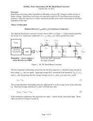
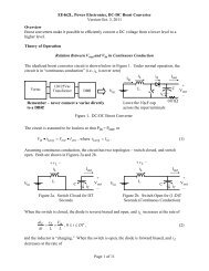
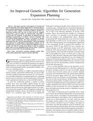
Fig. 1. Time domain for vehicle one in first row for three different sounds
and for vehicle 2 in the second row.
a classifier to find experimentally the classification rate.
Then support vector machine classifier is compared with
KNN classifier. The remainder of the paper is organized
as follows. Section II presents the related work. Section III
discusses the feature extraction methods. Section IV presents
Feature Extraction Performance. Section V describes the
experimental results. And finally, conclusions are discussed
in section VI.
II. RELATED WORK
Acoustic based vehicle classification differs mainly in
feature extraction approaches. In [5] Fast Fourier Transform
(FFT) and Power Spectral Density (PSD) are used to to
extract feature vectors. Similarly in [6] the first 100 of
512 FFT coefficients are averaged by pairs to get a 50-
dimensional FFT-based feature vector with resolution of
19.375 Hz and information for frequencies up to 968.75
Hz. Short Time Fourier Transform (STFT) is used in [7]
to transform the overlapped acoustic Hamming windowed
frames to a feature vector. Ref. [1] presents schemes to
generate low dimension feature vectors based on PSD, using
an approach that selects the most common frequency bands
of PSD in all the training sets for each class. Ref. [2]
proposes an algorithm that uses the overall shape of the
frequency spectrum to extract the feature vector of each
class. Principal component eigenvectors of the covariance
matrix of the zero-mean-adjusted samples of spectrum are
also used to extract the sound signature as in [8]. Ref. [9]
proposes a probabilistic classifier that is trained on the
principal components subspace of the short-time Fourier
transform of the acoustic signature. Wavelet preprocessing
provides multi-time-frequency resolution. Discrete Wavelet
Transform (DWT) is used in [10] and [11] to extract features
using statistical parameters and energy content of the wavelet
coefficients. Wavelet packet transform is also used to extract
vehicle acoustic signatures by obtaining the distribution of
the energies among blocks of wavelet packet coefficients like
in [3] and [4].
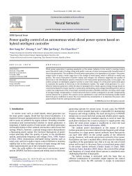
Fig. 2. Frequency distribution for vehicle one in first row for three different
sounds and for vehicle 2 in the second row. Fs is sampling frequency =4960.
Fw is FFT window size=512.
III. FEATURE EXTRACTION OF THE GROUND MOVING
VEHICLE’S SOUND
A. Feature Extraction using the PSD of the STFT
The goal is to develop a scheme for extracting a low
dimension feature vector, which is able to produce good
classification results. The first feature extraction technique of
acoustic signals in this paper is based on the low frequency
band of the overall spectrum distribution. The low frequency
band is utilized, because most of the vehicle’s sounds come
from the rotating parts, which rotate and reciprocate in a
low frequency, mainly less than 600 Hz. Sounds of moving
ground vehicles are recorded at the nodes at a rate of 4960
Hz. After the positive detection decision, a signal of event is
preprocessed as the following:
1) time preprocessing: DC bias should be removed by
subtracting the mean from the time series samples.
x i (n) =x i (n) − 1 N
N ∗ ∑
x i (n) (1)
n=1
.
2) spectrum analysis: Feature vector will be the median
of the magnitude of the STFT of a signal of event. It will be
computed as the following: the magnitude of the spectrum
is computed by FFT for a hamming window of size 512,
without overlapping.
X i (W )=FFT(x i (n)) (2)
After this, the spectrum magnitude is normalized for every
frame
X i (W )
X i (W )= ∑ K
W =1 X (3)
i(W )
where K is the window size. The median of all frames is
considered as the extracted feature vector.
X if (W )=median(X i (W )) (4)
571

0.16
0.14
v1
mean
standard deviation
0.14
0.12
v2
mean
standard deviation
1
0.95
SVM
KNN
0.12
0.1
0.9
Spectrum Power
0.1
0.08
0.06
0.04
Spectrum Power
0.08
0.06
0.04
Classification rate
0.85
0.8
0.75
0.02
0.02
0.7
0
0
0.65
−0.02
0 500 1000
ferquency(HZ)
−0.02
0 500 1000
ferquency(HZ)
6 7 8 9 10 11 12
Wavelet Level
Fig. 3. Acoustic spectra distribution of vehicle 1 and vehicle 2. To the left
is vehicle 1
Fig. 4. Classification rate vs. number of level for Wavelet Packet Transform.
Where the training set is equal three and k for KNN=3.
The mean of all frames could also be considered as the
extracted feature vector.
X if (W )= 1 Z
Z∑
X i (W ) (5)
i=1
where z = N/k. The first 64 points of the median of the
spectrum magnitude contain up to 620 Hz. This gives a 64
dimensional vector that characterizes each vehicle sound. We
compared feature extraction using the mean and the median.
The median gives better results, specially for noisy environments.
Fig.3 displays the acoustic spectra distribution of
vehicle 1 and vehicle 2. For the Unknown utterance, the same
steps are done, except one frame of FFT is considered as the
feature to be classified to reduce the cost of computation,
because this FFT computation is performed online. This can
be extended to have multiple frames, but this will increase
the cost of computation.
B. Feature Selection Using Wavlet Transform
Wavelet transforms provide multi-resolution timefrequency
analysis [12]. DWT approximation coefficients y
are calculated by passing the time series samples x through
a low pass filter with impulse response g.
∑
y(n) =x(n) ∗ g(n) =
∞ x(k)g(n − k).
k=−∞
The signal is also decomposed simultaneously using a
high-pass filter h. The outputs from the high-pass filter are
the detail coefficients. The two filters are related to each
other.
Wavelet packet transform can be viewed as a tree structure.
The root of the tree is the time series of the vehicle sound.
The next level is the result of one step of wavelet transform.
Subsequent levels in the tree are obtained by applying the
wavelet transform to the low and high pass filter results of
the previous step’s wavelet transform. The Branches of the
tree are the blocks of coefficients. Each block represents a
band of frequency. Feature extraction of acoustic signals is
based on the energy distribution of the block coefficients of
wavelet packet transform.
1) WPT Algorithm Steps: After the positive detection
decision, a one second time series is preprocessed as the
following:
• The wavelet packet transform is applied for this signal
then the energy of each block coefficients of the (L)
level is calculated. Fig.4 displays the relation between
the level number (L) of wavelet packet transform and
the classification rate for SVM and KNN classifiers
• This approach provides a vector of length = original
time series length /2 L . Which is considered the feature
vector.
Fig. 6 displays the blocks energy distribution for vehicle
1 and vehicle 2. In this paper we used classification rate
as the metric for the evaluation of the feature extraction
performance. But this metric depends on the classifier itself.
Thus, we compare the classification rate for two classifiers
as shown in Fig. 4 and Fig. 5. The classifiers performance
depend on the number of training sets. Fig. 5 shows the
relation between the number of training sets and the correct
classification rate. It is clear from the figures that the best
level length is eight for our specific data.
IV. FEATURE EXTRACTION PERFORMANCE
A. Separability Measures
Separability measures is a measure of class discriminability
based on feature space partitioning. Good feature vector
extractor provides close feature vectors for the same class,
and far feature vectors for distinct classes. The goal is to
have a feature extraction method that has high distance
between distinct classes and low distance within each class.
The metric is the separability ratio (sr), which is the ratio
between the intraclass distance and the average interclass
distance [13].
sr = D g
D l
(6)
572

1.2
1
SVM
KNN
0.6
0.55
Classification rate
0.8
0.6
0.4
Separability Ratio
0.5
0.45
0.4
0.35
0.2
0.3
0
3 3.5 4 4.5 5 5.5 6 6.5 7
Training set number
0.25
20 40 60 80 100 120
Feature Vector Length
Fig. 5. Classification rate vs. number of Training set for SVM and KNN.
Where (L) the number of level equals eight and k for KNN=3.
Fig. 7.
method.
Separability ratio vs. length of the feature vector for spectrum
0.1
vehicle 1
0.1
vehicle 1
0.1
vehicle 1
14
normailized Energy
Normailsed Energy
0.08
0.06
0.04
0.02
0
0 100 200
Blocks
vehicle 2
0.1
0.08
0.06
0.04
0.02
0
0 100 200
Blocks
normailized Energy
Normailsed Energy
0.08
0.06
0.04
0.02
0
0 100 200
Blocks
vehicle 2
0.1
0.08
0.06
0.04
0.02
0
0 100 200
Blocks
normailized Energy
Normailsed Energy
0.08
0.06
0.04
0.02
0
0 100 200
Blocks
vehicle 2
0.1
0.08
0.06
0.04
0.02
0
0 100 200
Blocks
Separability Ratio
12
10
8
6
4
2
0
2 4 6 8 10 12
wavelet packet level
Fig. 6. Wavelet block energy distribution for vehicle one in first row for
three different sounds and for vehicle 2 in the second row.
Fig. 8.
Separability ratio vs. level number for Wavelet method.
C∑ P i
∑n i
D g =
[(V ik − m i )(V ik − m i ) T ] 1 2 (7)
n
i=1 i
k=1
D g represents the average of the variances of distance within
all classes. V ik is the normalized feature vector. C is the
number of classes. P i is the probability of class i. n i number
of vectors in class i. m i is the mean vector for class i.
C∑
D l = P i [(m i − m)(m i − m) T ] 1 2 (8)
i=1
D l represents the average of the distances between all
classes. m is the mean for all classes.
∑ ni
k=1
m i =
V ik
(9)
n i
∑ C ∑ ni
i=1 k=1
m = V ik
(10)
n i
The smaller the ratio is the better the separability is. Which
means that the best feature selection scheme is the one that
decreases D g and increases D l . Fig. 7 shows the relation
between the separability ratio and the length of the feature
vector for spectrum method. Wavelet packet transform
feature selection method used in this research gives 0.5433
separability ratios in Fig. 8. While it is clear from Fig. 8
this ratio can be obtained with much less feature vector using
spectrum method. Spectrum method gives a separability ratio
less than 0.3 for the same feature vector length.
B. Correct Classification Rate
Classification rate not only depends on feature selection
methods but also on the classifier type. This drive us to
evaluate the performance of different classifiers.
1) KNN classifier: KNN is a simple and accurate method
for classifying objects based on the majority of the closest
training examples in the feature space. It is rarely used in
wireless sensor networks because it needs large memory and
high computation. In our experiments we set K to be three.
We use KNN as a benchmark to compare and evaluate the
performance of SVM.
2) Support Vector Machine (SVM): SVM is widely used
as a learning algorithm for classifications and regressions.
SVM classify data x i by class label y i ∈{+1, −1} given
573

a set of examples {x i ,y i } by finding a hyperplane wx + b
,x ∈ R n which separate the data point x i of each class .
g(x) =sign(wx + b) (11)
where w is the weight vector, b is the bias. SV M choose
the hyperplane that maximize the distance between the hyperplane
and the closest points in each feature space region,
which are called support vectors. So the unique optimal
hyperplane is the plane that maximize this distance
|wx i + b|/‖w‖ (12)
This is equivalent to the following optimization problem
min w,b ‖w‖ 2 /2, s.t. y i (w T x i + b) ≥ 1 (13)
For the cases that nonlinear separable, a kernel function maps
the input vectors to a higher dimension space in which a
linear hyperplane can be used to separate inputs. So the
classification decision function becomes:
sign( ∑
αi 0 y i K(p, p i )+b) (14)
i∈SV s
where SVs are the support vector machines. αi
0 andbare
a lagrangian expression parameters. K(p,p i ) is the kernel
function. It is required to represent data as a vector of a real
number to use SV M to classify moving ground vehicles.
Performance of SV M for vehicle classification based on
both feature extraction methods is also evaluated.
3) SVM Performance Evaluation: Cross validation is the
best way to evaluate the performance of SVM. The K-fold
scheme is used to determine the best kernel function based
on the highest correct classification rate. As in table I, three
kernels are compared: Linear, K(x i , x) =x i .x; Polynomial
K(x i , x) =(x i .x +1) d ; and Gaussian Radial Basis Function
(RBF), K(x i , x) = exp(−(||x i − x||)/(2σ 2 )). Fig.9and
Fig. 10 display the performance of SVM by plotting the
distances between the hyperplane surface and the feature
vectors using spectrum distribution and WPT respectively.
TABLE I
CORRECT CLASSIFICATION RATE FOR SPECTRUM METHODS
AND WAVELET USING SUPPORT VECTOR MACHINE WITH
DIFFERENT KERNEL FUNCTIONS AND DIFFERENT FEATURE
VECTOR LENGTH
Kernel ( Vector Length(spectrum)) ( Vector Length(wavelet))
32 50 64 32 64 128
Linear .969 .970 .978 .979 .970 .978
Gaussian RBF .720 .655 .642 .619 .611 .617
Polynomial D=3 .897 .860 .876 .888 .829 .860
V. EXPERIMENTAL RESULTS
In this paper, WDSN data base is used. It is available at
http://www.ece.wisc.edu/sensit. Fig. 1 and Fig. 2 show the
acoustic signals of the three different sounds for vehicle 1
and vehicle 2 in the time domain and the frequency domain
respectively. We use multiple real sounds of two different
Fig. 9. Distance for hyperplane surface vs. feature vector indices. Where
the first 22 indices are for vehicle one and the next 22 for vehicle 2.
Training set is =20 and data =44. Where features are extracted by Spectrum
distribution with vector length= 32. Circles and rectangles represent vehicle
1 and vehicle 2 respectively.
Fig. 10. Distance for hyperplane surface vs. feature vector indices. Where
the first 22 indices are for vehicle one and the next 22 for vehicle 2. Training
set is =20 and data =44. Where features are extracted by Wavelet Packet
Transform with vector length= 32. Circles and rectangles represent vehicle
1 and vehicle 2 respectively
military vehicles to evaluate feature extraction methods and
to train and evaluate the SVM classifier. All the parameters of
the feature extraction methods are evaluated. It is found that
the best level for WPT is eight. Feature vector length is evaluated
for the spectrum-based method and the kernel functions
for SVM. Table I shows that the best kernel function is the
linear function. Feature vectors with length of 32 give almost
the same correct classification rate as those with 64 and 128
features, which emphasizes our hypothesis that most of the
vehicle sound power is concentrated in the low-frequency
bands. K-fold and leave-one-out schemes were used to cross
validate the performance of SVM and KNN classifiers for
spectrum and wavelet methods of feature extraction. Correct
classification rates for vehicle 1 and vehicle 2 for a subset of
44 sounds are shown in table II for different feature vector
lengths, which provides a satisfactory results.
574

TABLE II
CORRECT CLASSIFICATION RATE FOR SPECTRUM METHODS
AND WAVELET USING SUPPORT VECTOR MACHINE AND KNN
CLASSIFIERS WITH DIFFERENT FEATURE VECTOR LENGTH
Feature Generation method SVM KNN
32 64 128 32 64 128
Spectrum Distribution .963 .963 .958 .818 .818 .750
Wavelet Packet Transform .961 .977 .978 .705 .930 .909
[12] H. liang Wang, W. Yang, W. dong Zhang, and Y. Jun, “Feature
extraction of acoustic signal based on wavelet analysis,” in the 2008
International Conference on Embedded Software and Systems Symposia
Volume 00, Jan. 2008.
[13] Wang, Lipo, Fu, and Xiuju, Data Mining with Computational Intelligence.
Springer Berlin Heidelberg, 2005.
VI. CONCLUSION
Feature extraction is a critical step for classification of
ground moving vehicles. This paper evaluates two common
feature extraction methods that are used in this field with
some modifications. The first method is based on spectrum
distribution and the second is based on Wavelet Packet
transform. The two methods are evaluated and compared
thoroughly. Evaluation criteria are based on the correct
classification rate and the separability ratio of the classes.
Both methods give almost the same correct classification
rates and separability ratios, while the first outperforms the
second in term of computation and memory resources, which
are critical in wireless sensor networks. Results proves that
most of the vehicle sound power is concentrated in the lowfrequency
bands. Experiment results shows that SVM is an
efficient ground vehicle classifier based on acoustic signals.
REFERENCES
[1] Y. Seung S., K. Yoon G., and H. Choi, “Distributed and efficient
classifiers for wireless audio-sensor networks,” in 5th International
Conference on Volume, Apr. 2008.
[2] S. S. Yang, Y. G. Kim1, and H. Choi, “Vehicle identification using
discrete spectrums in wireless sensor networks,” Journal Of Networks,
vol. 3, no. 4, pp. 51–63, Apr. 2008.
[3] A. Amir, Z. V. A., R. Neta, and schoclar Alon, “Wavelet-based acoustic
detection of moving vehicles,” Multidimensional Systems and Signal
Processing, vol. 57, no. 5, pp. 3187–3199, Apr. 2008.
[4] A. Amir, E. Huulata, V. Zheludev, and I. Kozlov, “Wavelet packet
algorithm for classification and detection of moving vehicles,” Multidin
Syst Sign Process, vol. 32, no. 5, pp. 31–39, Sep. 2001.
[5] H. Wu, M. Siegel, and P. Khosla, “Distributed classification of acoustic
targets wireless audio-sensor networks,” Computer Networks, vol. 52,
no. 13, pp. 2582–2593, Sep. 2008.
[6] ——, “Vehicle classification in distributed sensor networks,” Journal
of Parallel and Distributed Computing, vol. 64, no. 7, pp. 826–838,
July 2004.
[7] H. Xiao1, C. Cai1, Q. Yuan1, X. Liu1, and Y. Wen, Advanced
Intelligent Computing Theories and Applications. With Aspects of
Theoretical and Methodological Issue. Springer Berlin / Heidelberg,
2007.
[8] H. Wu, M. Siegel, and P. Khosla, “Vehicle sound signature recognition
by frequency vector principal component analysis,” IEEE Trans.
Instrum. Meas., vol. 48, no. 5, pp. 1005–1009, Oct. 1999.
[9] M. E. Munich, “Bayesian subspace methods for acoustic signature
recognition of vehicles,” in 12th European Signal Processing Conf),
Sep. 2004.
[10] C. H. C. K. R. E. G. G. R. and M. T. J, “Wavelet-based ground vehicle
recognition using acoustic signals,” Journal of Parallel and Distributed
Computing, vol. 2762, no. 434, pp. 434–445, 1996.
[11] A. H. Khandoker, D. T. H. Lai, R. K. Begg, and M. Palaniswami,
“Wavelet-based feature extraction for support vector machines for
screening balance impairments in the elderly,” vol. 15, no. 4, pp. 587–
597, 2007.
575