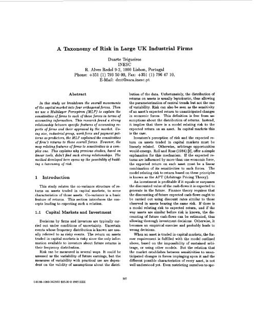
A taxonomy of risk in large UK industrial firms

A Taxonomy of Risk in Large UK Industrial Firms
Duarte Trigueiros
INESC
R. Alves Redo1 9-2, 1000 Lisbon, Portugal
Phone: +351 (1) 793 50 00, Fax: +351 (1) 796 47 10,
E-Mail: dmt@sara.inesc.pt
Abstract
In this study we breakdown the overall movements
of the capital market into four orthogonal forces. Then
we use a Multilayer Perceptron (MLP) to explain the
sensitivities of firms to each of these forces in terms of
accounting information. This research found a strong
relationship between specific features of accounting reports
of firms and their appraisal by the market. Using
size, industrial group, work force and payment patterns
as predictors, the MLP explained the sensitivities
of firm’s returns to these overall forces. However, the
map relating features of firms to sensitivities is a complex
one. This explains why previous studies, based on
linear tools, didn’t find such strong relationships. The
method developed here opens up the possibility of building
a taxonomy of risk.
1 Introduction
This study relates the co-variance structure of returns
on assets traded in capital markets, to some
characteristics of those assets. Co-variance is a basic
feature of returns. This section introduces the concepts
leading to expecting such a relation.
1.1 Capital Markets and Investment
Decisions by firms and investors are typically carried
out under conditions of uncertainty. Uncertain
events whose frequency distribution is known are usually
referred to as risky events. The return on assets
traded in capital markets is risky since the only information
available to investors about future returns is
their frequency distribution.
Risk can be measured in several ways. It could be
assessed as the variability of future earnings, but the
measures of variability with practical use are dependent’
on the validity of assumptions about the distri-
bution of the data. Unfortunately, the distribution of
returns on assets is usually leptokurtic, thus allowing
the parameterization of central trends but not the one
of variability. Risk can also be seen as the sensitivity
of an asset’s expected return to unanticipated changes
in economic forces. This definition is free from assumptions
about the distribution of returns. Instead,
it implies that there is a model relating risk to the
expected return on an asset. In capital markets this
is the case.
Investors’s perception of risk and the expected return
on assets traded in capital markets must be
linearly related. Otherwise, arbitrage opportunities
would emerge. Roll and Ross (1984) [9], offer a simple
explanation for this mechanism. If the expected returns
are influenced by more than one economic force,
the expected return on each asset must be a linear
combination of its sensitivities to such forces. The
model relating risk to return based on these principles
is known as the APT (Arbitrage Pricing Theory).
An investment is profitable if it equals or surpasses
the discounted value of the cash-flows it is expected to
generate in the future. Finance theory requires that
the discounting of future expected cash-flows ought to
be carried out using discount rates similar to those
observed in assets bearing the same risk. If there is
a model relating risk to expected return, and if the
way assets are similar before risk is known, the discounting
of future cash-flows can be estimated, thus
allowing thorough investment decisions. Otherwise, it
becomes an empirical exercise and probably leads to
wrong decisions.
When an asset is traded in capital markets, the former
requirement is fulfilled with the model outlined
above, based on the impossibility of sustained arbitrage,
or using other models. But the relation that
the market establishes between sensitivities to unanticipated
changes in forces impinging upon it and the
different possible characteristics of every asset, is not
well understood yet. Even restricting ourselves to spe-
0-8186-1060-3425/93 $03.00 0 1993 IEEE
587

cific groups of assets like industries, there is no available
guidance to relate expected returns to the features
of assets. As a consequence, it is impossible to
find out what makes assets similar before risk.
This study tries to fill this gap. It shows that it is
possible to build a taxonomy of risk. There is a strong,
though non-linear, relationship between assets’s characteristics
as perceived by the market and the way
they are traded.
1.2 Non-Diversifiable Risk
Assets are traded by what they are worth in the
market’s eyes. But the holders of traded assets are
not risking their wealth in a way that directly relates
to the risk of each asset they hold. Just by holding
many assets, investors smooth out a great deal of the
variability of their wealth. The only variability they
can’t avoid is the background movement of the whole
market.
This background movement is a unique time-history.
But it can be viewed as the result of a few orthogonal
forces or “factors’’, each one of them capturing
the largest dimension of the joint variability of returns
on all the traded assets. These factors are obtainable
from a representative number of time-histories of returns,
by decomposing their joint variability into main
orthogonal co-movements. Each factor is supposed to
be a linear combination of economic movements like
Inflation, Industrial Production, Risk Premium in the
market, and Interest Rate’s term structure growth.
After Ross’s seminal paper in 1976 [lo], the models
using arbitrage considerations to relate risk to return
(the APT), became present in the finance literature
but scarcely in the finance practice. The first signs
of their practical use only nowadays seem to emerge.
The reason for this delay may well be the immediate
interest of early models, based on one-dimensional
sensitivities to non-diversifiable risk (the Betas). It is
clear that, if a thoroughly calculated Beta really expresses
the co-variance of an asset’s return with the
whole movement of the market, then investors don’t
need anything else. The co-variance with the market
is the only portion of an asset’s variability that investors
will pay to avoid. Thus, it is also the only
piece of information they are likely to pay to know.
However, there are cases in which multi-dimensional
models based on arbitrage could become useful
for financial practice. Whenever a more precise understanding
of the way assets are traded is required, the
APT is the choice. This is the case for the appraisal of
productive commitments. It is also the case of studies
concerned with the market itself.
When searching for a taxonomy of risk, arbitrage
models seem promising. They are a breakdown of an
information content into features. They should allow
a better discrimination, each of the orthogonal forces
showing particular affinity towards some aspects of assets.
The APT offers the possibility of looking onto
an asset’s expected return from several points of view.
When the emphasis is not in the holder but in the
asset itself, the APT is the adequate instrument for
assessing the variability of returns. That’s why it’s
used here.
1.3 Stable and Fluctuating Features
The hypothesis that the market regards differently
the stable features of assets and the more fluctuating
ones, is a starting-point in our search for a taxonomy
of risk.
A rapidly growing body of research documents components
which can be forecasted in asset’s returns (see
for example Fama (1988) [4]). It is reasonable to divide
investors’s movements in two categories: Their
expectations, creating the predictable component of
returns, and their reaction to unanticipated events,
which creates the unpredictable one. Arbitrage considerations
(the APT) lead to models in which sensitivities
to unanticipated economic forces play a role:
Risk is about the second component of returns.
The expected component of returns mainly relates
to changes in accounting numbers. For example, an
increase or decrease in Earnings or Dividends influence
expectations (see, for example, Brown and Ball,
1967 [2]). However, the features of the firm aren’t
equally volatile: There are pieces of accounting information
that cannot vary swiftly as they reflect features
of the firm that are stable.
We think that the firm’s stable attributes are the
ones that mainly create in investors the sensitivity to
unanticipated forces. In fact, only stable features can
create sensitivity: The fluctuating ones aren’t sensitive
as they move along with the trends. For example,
the industrial group would explain to some extent the
sensitivity of investors to unexpected movements of
the economy, because firms cannot easily change sector
to face inflation or an excess of supply. Conversely,
less intrinsic features, like the financial structure or the
dividend policy, relate to trends and thus to expectations
observed in returns.
Hence, this study should search for relations between
the stable features of assets and their sensitivities
to market forces. We consider industry group, location,
size, operating leverage, labour and capital intensity,
payment pattern (hence, the short-term debt)
588

as candidates for explaining market sensitivity. Dividend
policy, capital structure, are less intrinsic. Earnings
could have both components.
1.4 Existing Research
This study isn’t a replica of an existing one, in
which an MLP is used instead of linear modelling
tools. It gives a new formulation to an old problem.
Such a formulation is partly possible because of the
MLP. It mainly concerns three areas of research: The
searching of correlations between characteristics of the
firm and risk, the building of proxies for Beta based on
acounting information, and the APT. Foster (1986) [5]
review them.
An early attempt to build a proxy for Beta using
accounting numbers is the one of Beaver, Kettler and
Scholes (1970) [l]. They achieved small but significant
correlations between accounting and market measures
of risk. Much research has also been published on the
correlation of operating leverage, gearing, size, with
Beta, the covariance of an asset’s expected return with
the background movement of the whole market. 30%
is a typical value for the proportion of variability of
returns explained by these models.
We would like to underline the fact that models
like those of “Fundamental Analysis” (which assumes
that each asset has an intrinsic value that can be determined
on the basis of earnings, dividends, capital
structure and potential growth) or “Equity Valuation”
(which focus on predicted earnings and dividends), are
not the kind of relation we are interested in here. Such
models calculate indexes reflecting trends observed in
individual histories of firms and use them to explain
the market reaction to the performance of those firms.
Since we focus on risk, that is, the unanticipated components
of returns, we are not trying to forecast returns
or other indexes.
2 Preliminary Processing of Data
This study brings together two sources of data.
Firstly, a large set of time-histories of returns on assets
traded in the London Stock Exchange, from which sensitivities
of a few of them to four orthogonal forces are
extracted. Secondly, the collection of accounting reports
of the assets whose sensitivities were extracted.
The sensitivities are the ones we use in the next section
as target or explained variables, both in the MLP
and in linear regressions. The accounting data will be
used as input.
2.1 Time-Histories of Returns
The assets selected for extracting sensitivities were
listed in the FTA All Shares Index. The reason for
using only listed firms relates to the decision of avoiding
infrequently traded assets. The known means for
circumventing the problems posed by infrequent trading
[3] would introduce in our experiment an extra
manipulation of information. For the same reason,
the use of daily or weekly returns was discarded. We
used monthly returns provided by the London Business
School, spanning a period of 15 years, from January
1974 to December 1988. Returns were calculated
as
Industry * * b I Industry N . b
Building - Materials I 11 I El ectronics I 9
Paper and Packing
Chemicals
Electrical
rt = log, (-) Pt + dt
Pt-1
in which pt stands for traded price in month t, pt-l
is the last traded price in month t - 1 and d* is the
dividend declared adjusted to a month-end basis. All
adjustments were based on the principle that the value
of a share is unaltered by a change in capital structure.
We used a total of 121 time-histories of assets for
the extraction of sensitivities. All of them were industries.
Included in these 121 firms were the 77 ones
whose accounting reports were to be related to their
sensitivities. The selection of the 77 final firms was
made on an industry basis. Only seven industries were
selected. Since one of our goals was the assessment of
the effect of industrial grouping, it didn’t seem appropriate
to gather in the same sample a large number of
industries. The selected ones were:
10 Textiles 10
15 FoodManuf. 13
9
All companies quoted on the London Stock Exchange
are classified into industrial groups according
to the Stock Exchange Industrial Classification
(SEIC). The above groups refer to the SEIC.
Given the returns of 121 industries during the referred
period, a Factor Analysis was performed on
their time-history taken as stochastic variables. The
aim was to rotate the co-variance matrix so that a
few minimum co-variance axis would emerge. Thus,
we obtained a breakdown of the cross-correlation of
time-histories into its four main components. In order
to maintain comparability with other APT studies we
used Maximum-Likelihood as the criterion for the extraction
of factors.
The resulting factors are supposed to be a linear
combination of a few economic forces impinging upon
589

the market. In our case the four main factors explained
47% of the variability of returns. Their Eigenvalues
(in percent of the explained variability) are:
39.5 0
42.5%
2.4% 44.9%
2.0% 46.9%
Sensitiv. to
Force N.
1
2
3
4
Skewness Kurtosis Mean St. Dev.
-0.88 -0.12 0.412 0.189
-0.48 0.19 0.269 0.124
0.40 0.60 0.263 0.148
1.88 1.03 0.184 0.126
Figure 1: The first factor’s sensitivities (Y-axis)
against U,, the relative size of firms (X-axis).
prices on the Paper industry. It is also very influential
for the Food industry, but in the opposite direction.
Factor 2 has a positive influence in Food Manufacturers
and Electronics. It has a negative or no effect on
the other industries. Factor 3 has a strong, negative,
influence on the Electronics industry. It is a positive
one for Food Manufacturers and Paper.
We also observed the correlations between the communality
associated with each firm, their loadings and
some features of these firms. The communality measures
the portion of variability of returns that are
explained by the factors. In our sample, it clearly
relates to Size and Earnings. This means that the
largest firms and the most profitable ones are also the
ones traded in a more similar, predictable, way. An
interesting study related to this issue is Roll’s “R2”
(1988) [8]. It is an empirical assessment of the variability
explained in stock returns by the market models.
Roll correlates the collection of R2 observed in several
kinds of market models with a few characteristics of
the firm.
Scatter-plots of features of firms against their sensitivities
were also observed as part of this preliminary
study. Correlations were observed between Size and
the first two factor’s sensitivities. The correlation between
Size and the first one is non-linear (see figure 1
on page 4). The second one exhibits a negative, linear,
correlation with size but industrial groups form
visible clusters. Also Gross Funds From Operations
and Inventory show significant correlation with some
sensitivities.
2.2 Accounting Reports
Factor 1
35.4%
Factor 2 Factor 3 Factor 4
39.9% 43.1% 3.4%
Using the convention of calling “positive” to influences
which are above the expected and “negative”
otherwise, we can say that Factor 1 strongly influences
Accounting raw data, as found in databases containing
collections of annual reports of firms, can be
viewed as statistical variables. Each firm is a case. For
a given item, say, Fixed Assets or Sales, a collection
of reports from the same year forms a cross-sectional
sample. The probability density function governing
590

such variables is the lognormal one. Items belonging
to the same report share, in cross-section, most of
their variability. This is caused by the prevalent effect
of size. Size is an important piece of information
but its effect isn't directly measurable. However, it is
possible to isolate it by building, inside each report,
averages of a few positive-valued items like Net Worth,
Wages or Sales. In this way, we self-smooth the particular
scatter of each item so that only the common
one remains.
Thus, considering a group of accounting items,
zf , i = 1, M, from the jth report, we explain their variability
as the result of an effect, uj , common to them
all, plus the residuals, E:, particular to each item:
log.; - p1 = uj +E;
10gzj - p2 = uj + Ej
logx -pM
= uj +E
The pi are the expected values of logz'. The average
of the 1,. . . , i, . .-, M mean-adjusted items case
by case yields, for report j ,
. M
1 1
M
uj = - C(l0gzj -pi) - +€; +. ..+E)
i=l
Since an average of independent random deviates
tends to zero with 1/M,
Gr. Fundsfr. Operat. NW Net Worth
CA Current Assets Current Liabil.
Inventory
Sales
Number of Empl. W Wages
Table 1: List of accounting items used in this study
and their abbreviations.
denominator is the statistical effect of size and the
numerator is the deviation of item i from the standard
in its industry. Such ratios reflect the proportion to
which the item in the numerator departures from the
expected for firms of that size. That is, the are
size-adjusted Sales, Working Capital and so on. Apart
from rendering Gaussian inputs, the use of log space
makes the similar to proportions: The deviations
from size they assess are independent of scale and unit
of measure.
3 TheMethod
We modelled sensitivities in terms of accounting information,
firstly using linear regressions and then the
MLP. In both cases the training sets were the same.
Since the four targets are almost orthogonal there is
nothing to be gained from showing them jointly to
the modelling tool. Hence, we built four independent
MLPs, each one for explaining one sensitivity.
3.1 Input Variables
for large enough M. Once obtained, U allows the assessment
of the ci particular to each item:
E: =logzf.-pi-uj (1)
In this study, the estimated U was obtained as
U = $[logs + log NW + logW + logN
+ log D + log CA + log CL]
(2)
The meaning of the abbreviations can be found in table
l. The log items were mean-adjusted separately by
industry and by year before being used in formula (2).
Thus, the industry and year effects aren't present in
these variables. A more detailed characterisation of
the statistical behaviour of accounting data can be
found in Trigueiros (1992) [15].
We used the E ~ along , with our proxy for size, the
uj, as input variables to explain sensitivities. Notice
that the E" are the logarithm of ratios in which the
Table 2 on page 7 shows the 17 input variables used
both in the linear regressions and in the MLP. Nine of
them are the E ~ obtained , from applying formula (1)
to accounting items. One is our proxy for size, the
U,, as calculated by formula (2). The remaining seven
are dummy variables taking the value 1 when a case
belongs to a particular industry and 0 otherwise.
The selection of the set of nine items was a result
of an exploratory study, similar to the one presented
here but involving a larger number of items and different
topologies. The penalization of small weights,
to be described in section 3.2, allowed the elimination
of non-significant input variables.
The accounting data were drawn from the Micro-
EXSTAT database of company financial information
provided by EXTEL Statistical Services Ltd, which
covers the top 70% of UK industrial companies. As
mentioned above, we used the reports of 77 firms
matching the selected sensitivities. For each firm,
four years of accounting reports were collected: 1983
59 1

Figure 2: Schematic representation of the used MLP.
to 1986. Each example in the training set contains
the accounts of one firm for one of these years and
having as target one sensitivity. Therefore, there are
77 x 4 = 308 examples.
3.2 The MLP
In many MLP applications the problem is one of
classification. In this case it was one of regression.
The only difference, in what concerns the MLP, is that
linear transfer functions must be used in the output
layer of nodes and that the adequate success criterion
is Least-Squares minimization, not Likelihood maximization.
The topology of the MLP and the input variables
were similar in the four cases (see a schematic representation
in figure 2). There were 17 input nodes,
corresponding to 17 input variables. The unique hidden
layer had four nodes and the output layer had a
linear transfer function. This topology seems austere.
But since the number of cases in the training set was
small, the number of parameters in the models had to
be small as well. The characteristics which make our
MLP different from the standard algorithm (Rumelhart
et all. 1986 [ll]) can be summarized as:
e The use of two samples, one to learn and another
one to assess the classification performance, along
with incomplete training.
e Penalization of small weights, as described by Trigueiros
and Berry (1991) [16].
e Learning rates particular to each weight as described
in Silva and Almeida (1990) [12].
We now comment on these characteristics. The first
one relates to improvements in the ability to generalise.
It is a particular implementation of a known
procedure, the Cross-Validation (see Stone 1978 [14]).
In order to obtain an estimate of the generalisation
capacity of a model, the original samples were divided
randomly into two sub-samples. Models were constructed
with one sub-sample, the training set, and
a check carried out with the other one, the test set.
Since the outcomes were continuous-valued, the adequate
measure of quality of fitting was the proportion
of explained variability, R2, corrected for the degrees
of freedom engaged. All reported results concern the
test set, not the training set. That is, they were obtained
by measuring the rate of explained variability
in the half-set not used for training. The performance
on the set used for training depends solely on the number
of free parameters and can be increased simply by
introducing more nodes on the net. Therefore such
results are uninteresting.
The randomization leading to the division into two
samples - the test and the training set - was carried
out by firms on an industry basis. Thus, the two
resulting groups of firms didn’t yield large differences
in their proportion of cases for each industry. The
training set contained 213 of the firms.
Since the MLP seeks an optimum iteratively, we
can stop its training when an optimum is obtained
in the test set rather than in the training set. We
thus prevent this powerful algorithm from over-fitting
the data. The Back-Propagation algorithm seeks the
modelling of progressively smaller or less important
features of the relation, during the learning process.
Firstly, broad features are accounted for: The mean,
a linear trend. Then, more detailed ones are modelled.
Hence, the effective degrees of freedom the MLP engages
can be viewed as increasing during learning. Assuming
that the topology of the net contains plenty of
free parameters, the MLP will be able to model, not
only the desired features but also the undesirable random
uniqueness of a particular sample. We prevent
it from doing this by stopping the process before finishing.
The appropriate moment for stopping is when
the results, as measured by the test set, are optimal.
For a good topology, the fact that the learning stops
before a minimum is reached in the learning set clearly
enhances generalisation.
Finally, we introduced during training a penalization
of weights smaller than 1 in order to enhance interpretability.
If the input variables were very differently
scaled, weights smaller than 1 could just mean
that the MLP was trying to scale down a particular
variable. Since the input to the MLP are meanadjusted
and have similar standard deviations, the
only reason for any such weights to remain small
throughout the learning is to try to diminish the importance
of one variable to the output of the node it
592

Input variable
Chemical
Electronics
Size )
Textiles (d-y 1
Wages
(e:)
Current Assets (E: 1
Debtors
(cl)
Electrical
(dummy)
Net Worth (E’ 1
Paper and Packing
Building Materials
Sales
(e’)
Fixed Assets (E’ )
Food Manufacturers (d-y)
Gross Funds From Ops. (E’)
Debt
(E’)
Inventory (4
Number of parameters engaged Total
Model 1 Model 2 Model 3 Model 4
3 1 1 1 6
2 3 1 6
2 2 2 6
2 2 2 6
3 1 2 6
3 1 1 5
2 1 2 5
1 1 2 1 5
3 1 1 5
3 1 1 5
3 1 4
1 2 3
1 1 2
1 1 2
1 1 2
1 1
1 1
Table 2: The number of parameters (first hidden layer) engaged during the training of the four MLP, by input.
belongs to. In the MLP, each node acts as a modelling
unit with a certain amount of free parameters. The
same output can be obtained with very different combinations
of weights. Small weights connecting inputs
with the first hidden layer appear when a node tries
to weaken the contribution of a variable. If we introduce
a penalization of such weights during the training,
as the correction of weights is proportional to the
input variables, small weights tend to remain small.
In the same way, large weights tend to have their values
strengthen. The final result is a contrasted set of
weights: The first layer now contains only very large
or very small weights. The information concerning
the modelled relation is concentrated in a few weights
instead of distributed by all of them [16].
Notice that we never tried this method with the
simple Back-Propagation. Each one of the weights in
our MLP has its own increment, adjusted as described
in Silva and Almeida (1990) [12]. Other popular methods
for pruning the MLP are the “Skeletonization” [7]
and “Optimal Brain Damage” [6]. However, the first
one is intended to reduce the number of nodes, not
the one of weights. The second one is too general for
this task.
4 The MLP Versus Linear Regression
Table 2 shows, for each one of the four models, the
number of non-zero weights in the first hidden layer,
when the training finished. The remaining ones were
set to zero by the algorithm described above and play
no role in the modelling. The non-zero weights are the
parameters of the first hidden layer engaged during
the training of the MLP. Since the number of nodes in
the first hidden layer was four, the maximum number
of parameters per input variable that the MLP could
engage in the modelling process would be four as well.
This never happened. The training started with 68
free parameters and finished with 29 remaining ones
(the first model), 20 (the second), 9 (the third), and
12 (the fourth).
The number of parameters engaged is a rough measure
of the complexity of the relation. Size and Wages
engage a total of six parameters. Debt and Inventory
merely engage one. In general, the dummy variables
engage more parameters than items. Next table compares
the proportion of variability, R2, explained by
all models, when using linear regressions (OLS) and
the MLP.
R’ I Model1 I Model2 I Model3 I Model4
MLP I 71% I 48% I 69% I 36%
I OLS I 60% I 42% I 52% I 21% I
The comparing of the R2 achieved by the MLP with
those of linear regressions lead us to conclude that the
MLP made a significant improvement in capturing the
relation. In next section we shall see why: Such a
relation contains higher order effects and other sources
of complexity.
5 Exploring the Models
This section describes how the exploring of the four
models was carried out. We used an “other things being
equal” approach. It consisted of varying one of the
inputs at a time, and maintaining all the others fixed
593

n.
05
0.3
Size
0.1
-1.6 -12 na 4.4 0.4 0.8 12 1.6
0.a , 1
0.7
0.6
0.7 1
Gr. Funds
0.3
03
0.1
na
Figure 3: The first factor’s sensitivity to Size (above)
and to Gross Funds From Operations (below) as predicted
by the MLP.
Figure 4: The first factor’s sensitivity to size-adjusted
Current Assets (above) and Debtors (below) as predicted
by the MLP.
in their mean values. The observed outputs could then
be compared.
The chosen approach is the only one available in
this case. The model the MLP yields is far too complicated
for direct interpretation. The used procedure
allows an effective look into what the model
does. However, in some cases, the “other things being
equal” technique yields misleading results since the
other things cannot remain equal in the real world.
We firstly comment on the simplest relations - the
ones which are linear regarding industrial grouping.
Then, we comment on those cases in which the model
shows industries reacting in different directions to the
same force.
Figure 3 shows, for a few industries, the relation
modelled by the MLP when explaining the first factor’s
sensitivity to Size (above) and Gross Funds From
Operations (below). Similar patterns were obtained
for Sales and Long Term Debt (a negative correlation).
Each line represents an industrial group. Notice
that, since we used size-adjusted items as input
variables (the E ~ formula , l), a value of zero means the
expected for firms of that size. Values larger than zero
mean Sales or Gross Funds above the expected.
Electronics is the industry whose size has the
largest sensitivity to the first economic force, while
Building Materials is the one with the smallest. However,
since in Factor Analysis the sign of the factors is
arbitrary, the displayed curves yield a coherent view
but not one directly comparable with studies based
on correlations with Beta. For example, the trends
we observe in the case of the first factor are the inverse
of the ones Beaver, Ketler and Scholes (1970) [l]
obtained for similar variables.
The first factor rewards positive features of the firm
and penalizes Debt. None of the displayed curves deserved
from the MLP the engagement of many parameters
as these are easy-to-build relations. The second
factor rewards Wages, Debtors and penalizes Earnings.
But some industries are more sensitive than others.
Again, remember that the meaning of Wages or
Sales being large is that they are large given the size
of the firm. The third factor’s sensitivities reward Net
Worth and penalize Fixed Assets. Finally, the fourth
factor’s sensitivities penalize Size and Debtors and reward
Inventory but in a non-linear way.
So far, we described the cases in which the sensitivities
of all industrial groups react in the same direction
to the same orthogonal force. If we examine the
number of parameters engaged by the MLP we notice
that, except for Size, none of the relations commented
above deserved the use of many degrees of freedom.
Size needed more degrees of freedom as it is a strong,
non-linear though monotonic relation. But it is similar
across industries.
We now study a few cases in which the MLP put a
great effort. The first one is displayed in figure 4 on
page 8. It is clear that the first factor’s sensitivities
reward Debtors for industries like Textiles or Paper
and penalize it for industries like Food Manufacturers.
The interaction of Current Assets with the first
force is particularly awkward. It seems as if there is a
penalization of the values expected for a given size in
industries like Chemicals and Building Materials along
with a rewarding of the same situation in Electronics
and Food.
594

Factor 2 also displays this higher-order behaviour.
Figure 5 on page 9 shows the complicated pattern of
its relation with Net Worth and Size. Again, industries
seem to be affected in different directions by the
same market force. It rewards Net Worth if it is the
expected one for firms of that size, in industries like
Textiles and Paper. But it penalizes the same situation
if the industry is Food. In the Electronics industry
this force simply rewards capital. A standard size
is rewarded by this factor if the industry is Textiles. It
is penalized if it is Food. Small firms are, in general,
rewarded by this factor. But there is one exception,
Textiles. On the contrary, in the case of Electronics
firms, the smaller the better - with regard to the
second factor.
The third factor’s sensitivities reward Wages if near
the expected, penalizing both higher and smaller ones.
Fixed Assets of the Electronics industry seem not to
be affected by this force.
6 Towards a Taxonomy of Risk: Discussion
and Conclusions
The sensitivities of assets to unanticipated market
forces seem to be closely related to features identifiable
and measurable in assets. Size and industrial
grouping are the characteristics of assets which mostly
explain sensitivities. Deviations from the expected for
size in Wages, Net Worth and Sales, along with the
short-term structure, also relate significantly to sensitivities.
However, the relation between sensitivities
and features is complex. The industrial grouping interacts
with features like Net Worth, Current Assets
or size. The same market force reacts in opposite directions
to the same feature in different industries.
To some extent, particular forces impinge upon specific
features. The fourth orthogonal force is the only
one relating to Inventory. The third one relates mainly
to Wages and the second one to Net Worth. The first
and second forces’s sensitivities react to Size in opposite
directions. All of them recognize industrial grouping
but the fourth one to a small extent.
The ability of the MLP to model higher order relations
achieved a significant improvement in our knowledge
of the way the market recognizes and rewards
assets. However, the results were obtained from less
cases than desirable and further experiments involving
more firms should be carried out.
The fact that our sample is a dated one - it belongs
to a period of stability and expansion - seems fortunate.
The modelling of these relations would be diffi-
Net Worth
0.05 ’
-1:s -12 0’s d 4 d 0:4 0.3 12 1.’6
Figure 5: The second factor’s sensitivity to sizeadjusted
Net Worth (above) and Size (below) as pre
dicted by the MLP.
cult to carry out in data from recessive periods as the
number of non-traded assets would greatly increase.
The firms used are also from a particular set. They are
large and frequently traded. They were drawn from
well known and homogeneous industries. Our results
refer to such set and shouldn’t be extrapolated. The
behaviour of returns on less important assets is an interesting
issue but there isn’t enough information to
clarify it using statistical methods.
There are other studies of this kind in the accounting
and finance literature. Though they found significant
correlations between accounting and market
risk variables, their proportions of explained variability
were smaller than ours. The reasons for this are
several: Instead of using ratios, we defined an input
space based on a statisticaly sound analysis. It may
well be that such an input is suited for modelling to
an extent so far unattained by other studies. Also, we
modelled co-variability, not indexes extracted from individual
histories. Thus, we avoided using pieces of information
the market regards as predictable. Most of
the existing studies use earnings, dividends and their
standard deviations to predict Betas. But these variables
are, to some extent, predictable. They relate
to the policy and quality of management. They have
little in common with unanticipated components of
overall forces. We have shown that the way investors
react to unanticipated changes mainly depends on stable
characteristics of assets. Finally, we modelled four
different points of view, not just one, thus obtaining
a better scanning of the variability of returns, and we
used non-linear tools for modelling relations that are
complex.
It seems now clear that there is room in finance re-
595

search for the use of MLPs. They apportion significant
improvements in the amount of explained variability
in crucial problems as they model higher order relations
without damaging generalisation.
Our results also show that it is possible to build,
for each group of assets, a taxonomy of risk in terms
of their characteristics. Expected returns can then be
calculated on the basis of such characteristics allowing
a less blind discounting of future cash-flows. For
example, if a productive commitment is to be undertaken,
the models produced by the MLP could be fed
with its budgeted numbers. As a result they would
yield four sensitivities. Then the APT would predict
its return based on these sensitivities.
Finally, it seems also possible to achieve a better
understanding of the forces impinging upon the market
by examining the features of firms and industries
affected by each force.
Acknowledgements: We acknowledge the guidance
and continued support of Professor Luis B.
Almeida at INESC, Lisbon. The experiments described
in this study and some developments that followed,
were carried out in the University of East Anglia
in the UK. We thank Professor Robert €I. Berry
for his valuable support.
References
W. Beaver, H. Kettler, and M. Sholes.
The association between market-determined and
accounting-determined risk measures. The Accounting
Review, pages 654-682, October 1970.
P. Brown and R. Ball. Some Perliminary Findings
on the Association Between the Earnings of
a Firm, its Industry, and the Economy. Empirical
Research in Accounting: Selected Studies, 1967.
Suplement to Journal of Accounting Research.
E. Dimson. Risk measurement when shares are
subject to infrequent trading. Journal of Financial
Economics, 7:197-226, 1979.
E. Fama and R. French. Dividend yields and expected
stock returns. Journal of Financial Economics,
22:3-25, 1988.
G. Foster. Financial Statement Analysis.
Prentice-Hall, 1986.
Y. LeCun. Optimal brain damage. In Neural Information
Processing Systems, volume 1. Morgan
Kaufmann, Denver 1990.
M. Mozer and P. Smolensky. Skeletonization: A
technique for trimming the fat from a network via
relevance assessment. In Neural Information Processing
Systems, volume 1. Morgan Kaufmann,
Denver 1988.
R. Roll. R2. The Journal of Finance,
XLIII(2):541-567, July 1988.
R. Roll and S. Ross. The arbitrage pricing theory
approach to stratergic portfolio planning. Financial
Analysts Journal, pages 14-26, May 1984.
S. Ross. The arbitrage theory of capital asset pricing.
Journal of Economic Theory, 13:341-360,
1976.
D. Rumelhart, G. Hinton, and R. Williams.
Learning internal representations by error propagation.
In Parallel Distributed Processing, volume
1. The MIT Press, 1986.
F. Silva and L. Almeida. Acceleration techniques
for the backpropagation algorithm. In Neural
Networks. EURASIP Workshop, Sesimbra, Portugal,
1990. L. B. Almeida and C. J. Wellekens
(Eds.), Springer-Verlag.
G. Snedecor and W. Cochran. Statistical Methods.
Iowa State University Press, gth edition,
1965.
M. Stone. Cross-validation: A review. Math.
Operationsforsch. Statist., Ser. Statistics, 9( 1),
1978.
[15] D. Trigueiros. The Cross-Sectional Characterization
of Accounting Data. Technical Report,
ISCTE, Lisbon, Portugal, 1992.
[IS] D. Trigueiros and R. Berry. The application
of neural network based methods to the extraction
of knowledge from accounting reports. In
E. Nunamaker and R. Sprague, editors, Organisational
Systems and Technology: Proceedings of
the 24th Hawaii International Conference on System
Sciences, pages 136-146. IEEE Computer Society
Press, 1991.
596