Homework #2 - UCSD VLSI CAD Laboratory
Homework #2 - UCSD VLSI CAD Laboratory
Homework #2 - UCSD VLSI CAD Laboratory

You also want an ePaper? Increase the reach of your titles
YUMPU automatically turns print PDFs into web optimized ePapers that Google loves.
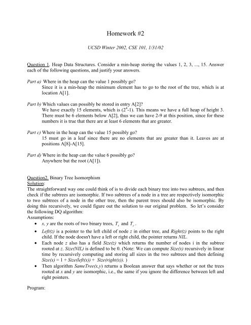
<strong>Homework</strong> <strong>#2</strong><br />
<strong>UCSD</strong> Winter 2002, CSE 101, 1/31/02<br />
Question 1. Heap Data Structures. Consider a min-heap storing the values 1, 2, 3, ..., 15. Answer<br />
each of the following questions, and justify your answers.<br />
Part a) Where in the heap can the value 1 possibly go<br />
Since it is a min-heap the minimum element has to go to the root of the tree, which is at<br />
location A[1].<br />
Part b) Which values can possibly be stored in entry A[2]<br />
We have exactly 15 elements, which is (2 4 -1). This means we have a full heap of height 3.<br />
There must be 6 elements below A[2], thus we can have 2-9 at this position, since for these<br />
numbers it is true that there are at least 6 elements that are greater.<br />
Part c) Where in the heap can the value 15 possibly go<br />
15 must go in a leaf since there are no elements that are greater than it. Leaves are at<br />
positions A[8]-A[15].<br />
Part d) Where in the heap can the value 6 possibly go<br />
Anywhere but the root (A[1]).<br />
Question2. Binary Tree Isomorphism<br />
Solution:<br />
The straightforward way one could think of is to divide each binary tree into two subtrees, and then<br />
check if the subtrees are isomorphic. If two subtrees of a node in a tree are respectively isomorphic<br />
to two subtrees of a node in the other tree, then the parent trees should also be isomorphic. By<br />
doing this recursively, we could figure out the solution to our original problem. So let’s consider<br />
the following DQ algorithm:<br />
Assumptions:<br />
• x, y are the roots of two binary trees, Tx<br />
and<br />
T y<br />
.<br />
• Left(z) is a pointer to the left child of node z in either tree, and Right(z) points to the right<br />
child. If the node doesn't have a left or right child, the pointer returns NIL.<br />
• Each node z also has a field Size(z) which returns the number of nodes i in the subtree<br />
rooted at z. Size(NIL) is defined to be 0. (Note: We can compute Size(x) recursively in linear<br />
time by recursively computing and storing all sizes in the two subtrees and then defining<br />
Size(x) =1+Size(left(x)) + Size(right(x)). )<br />
• Then algorithm SameTree(x,y) returns a Boolean answer that says whether or not the trees<br />
rooted at x and y are isomorphic, i.e., the same if you ignore the difference between left and<br />
right pointers.<br />
Program:
SameTree(x, y: Nodes): Boolean;<br />
IF Size(x) ≠ Size(y) THEN return False; halt.<br />
IF x=NILTHEN return True; halt.<br />
IF SameTree(Left(x), Left(y))<br />
THEN return SameTree(Right(x), Right(y))<br />
ELSE return (SameTree(Right(x), Left(y)) AND SameTree(Left(x), Right(y)));<br />
Time analysis:<br />
ÿ If the two trees are of different sizes, the program immediately returns false.<br />
ÿ If Tx<br />
and T y<br />
are of both size n:<br />
If the subtrees of Tx<br />
and T y<br />
are of different size l and r=n-l-1, then we do at most<br />
one recursive call (suppose it doesn’t return false immediately) of size l and one of<br />
size r.SowehaveT(n) ≤ T(l) + T(n-l-1) + O(1).<br />
If all subtrees are of equal size, then all of them should be size (n-1)/2, thus we have<br />
T(n) ≤ 3T(n/2) + O(1), because we will make at most 3 recursive sub-calls of size<br />
log 3<br />
less than n/2. This seems to be the worst case, and we get T(n) = O( n 2<br />
) according<br />
to the Master method.<br />
Now we conjecture this is true, that is, this is also true with the case when the subtrees are<br />
of different size l and r. We prove it by induction.<br />
3<br />
Claim: T(n) ≤ c n log 2<br />
Base: choose appropriate c, the claim is true when n =1.<br />
Induction: hypothesis: assume the claim is true for all 1 ≤ n ≤ k<br />
Now let n=k+1, apply the induction hypothesis, we have<br />
log 3<br />
T(n) ≤ cl 2<br />
3<br />
+c( n − l −1) log 2<br />
+ c<br />
log 3 1<br />
≤ cl 2 −<br />
3 1<br />
l +c(n-l-1) ( 1) log 2 −<br />
n − l − + c<br />
log 3 1<br />
≤ (cl+ c(n-l-1)) 2 −<br />
n + c<br />
log 3 1<br />
≤ (c(n-1)) 2 −<br />
n + c<br />
log 3<br />
≤ c n 2 log 3 1<br />
-c 2 −<br />
n + c<br />
log 3<br />
≤ c n 2<br />
(because n ≥ 1)<br />
log 3<br />
Therefore, by induction, T(n) ≤ c n 2<br />
is true for all n. So the runtime of this DQ algorithm<br />
log 3<br />
should be T(n) = O( n 2<br />
).<br />
By the way, there is another non-DQ solution to this problem in linear time. Briefly, first transform<br />
both trees to left-heavy (or right-heavy) form, that is, the bigger subtree is always on the left (or<br />
right). This can be done using several O(n) DFS traversals. Then by using DFS compare the size of<br />
subtrees in all levels, we will get the answer.<br />
Question 3. Median of two sorted lists: CLRS 9.3-8 (2nd edition pg. 193).<br />
Solution:<br />
We have to take advantage of the fact that we know that X and Y are sorted. If X[5] is the median it<br />
means that 4 elements in X are less than the median and n-5 elements are greater. This then implies<br />
that the remainder of the elements less than the median are in Y[], so we know that in Y[] the first n-<br />
4 elements are less than the median and the last 5 elements are greater than the median. What we
need to do is to perform a binary search for the median in one of the arrays. The search is guided by<br />
the contents of the other array. In particular, if we claim that the median is the i-th element in X,<br />
then we have three cases. Case 1) If X[i] =Y[n-i+1] then the claim is true. Case 2) If X[i] Y[n-i+1] then the claim is false and the actual median is to the left of i in X, orto<br />
the right of (n-i+1) in Y. The following is a recursive DQ algorithm, which essentially is a<br />
modified binary search in a sorted list.<br />
FindMedian (X[1..n], Y[1..n])<br />
{<br />
n = length(X)<br />
if (n ÿ 2)<br />
Z = Merge(X[1..n], Y[1..n])<br />
return Z[2]<br />
end<br />
c = floor((n+1)/2))<br />
if (X[c] == Y[n-c+1])<br />
return X[c];<br />
if (X[c] > Y[n-c+1])<br />
return findMedian(X[1..c] , Y[n-c+1..n]);<br />
return findMedian(X[c..n], Y[1..n-c+1]);<br />
}<br />
The algorithm is essentially the same as binary search. The recurrence relation for it is: T(n) =<br />
T(n/2) + O(1). Using the Master Method we get that the running time of this proposed algorithm is<br />
ÿ(lg n). Since the running time of the Merge function is O(n), the call to it in the base case does not<br />
affect the overall running time complexity of the main algorithm since the arguments of Merge are<br />
arrays of constant length (i.e., length
BEGIN<br />
{ IF thex field of the head of ListA is less than that of ListB<br />
THEN Currentx ← the x field of the head of ListA,<br />
CurrentHeightA ← the y-field of the head of ListA,<br />
Append (Currentx, Max(CurrentHeightA, CurrentHeightB)toKeypoints,<br />
Delete the head of ListA.<br />
ELSE Currentx ← the x field of the head of ListB,<br />
CurrentHeightB ← the y-field of the head of ListB,<br />
Append (Currentx, Max(CurrentHeightA, CurrentHeightB)toKeypoints,<br />
Delete the head of ListB.<br />
}<br />
8. IF ListA = NUL<br />
THEN append ListB to Keypoints.<br />
ELSE append ListA to Keypoints<br />
9. RETURN Keypoints.<br />
In this algorithm above, line 3 and 4 is the “divide” part, while line 5 to 8 is the merge (conquer)<br />
part. The merging is like the merge sort, just go through the already sorted ListA and ListB, sothe<br />
runtime of this part is O(k) (k is the minimum of the sizes of the two list). Therefore, according to<br />
the Master Theorem, T(n) = 2T(n/2) + O(n), so the time complexity of this DQ algorithm is T(n) =<br />
O(nlogn).<br />
Question 5. Stooge sort: CLRS 7-3 (2nd edition pg. 161).<br />
Solution:<br />
Part a) We will prove by induction that Stooge sort correctly sorts the input array A[1…n]. The<br />
base case is for n=2. In this case the first two lines of Stooge sort guarantee that a bigger element<br />
will be returned in a position following that of a smaller element. Thus, Stooge sort correctly sorts<br />
A when n=2. The inductive case happens when n 3. Then, assume by inductive hypothesis that<br />
the recursive call to Stooge-sort in line 6 correctly sorts the elements in the first two-thirds of the<br />
input array A, and let A’ be the array thus obtained. Also, assume by inductive hypothesis that the<br />
recursive call to Stooge-sort in line 7 correctly sorts the elements in the last two-thirds of the array<br />
A’, and let A’’ be the array thus obtained. Finally, assume by inductive hypothesis that the recursive<br />
call to Stooge-sort in line 8 correctly sorts the elements in the first two-thirds of the array A’’, and<br />
let B be the (final) array thus obtained. Now we need to prove that at the end of the algorithm, the<br />
array B is sorted. To prove this, we just need to prove that for any two elements A[i]
will be swapped. Here we have some other cases. First, if A[j] andA[i] are both in the first twothirds<br />
of the input array A, then they will be swapped in the recursive call in line 6 (which is<br />
correct by inductive hypothesis) and will not be swapped again in the following recursive<br />
calls (again, by the inductive hypothesis). Second, if A[j] andA[i] are both in the last two-thirds of<br />
the input array A, then they will be swapped in the recursive call in line 7 (which is correct by<br />
inductive hypothesis) and will not be swapped again in the following recursive call (again, by the<br />
inductive hypothesis). Finally, if A[j] is in the first one-third of the input array A and A[i] isinthe<br />
last one-third of the input array A, then we claim that their position are swapped either in the<br />
recursive call in line 7 or in the recursive call in line 8. In fact, assume their positions are not<br />
swapped in the recursive call in line 7. This means that after the execution of the recursive call in<br />
line 6 (which is correct by inductive hypothesis) the position of A[j] in array A’ is still in the first<br />
one-third and moreover, at least all the elements in the second third of A’ are greater than A[j].<br />
Then we have that since these elements are greater than A[j], then they are greater than A[i] (since<br />
we assumed A[i]
Step 5: Shift all the points in the list back to the original plane by x=x+ x m<br />
,y=y+ y m<br />
output this final list of maximal elements. The time complexity is O(n).<br />
Therefore, the total of this algorithm runtime T(n) = O(nlogn).<br />
,and<br />
Question 7. Water Jugs: CLRS 8-4 (2nd edition pg. 179).<br />
Solution:<br />
Part a) A simple deterministic algorithm to group the jugs in pairs is the following. Select a jug<br />
from the blue set. Compare it with every red jug and find its pair. Do this for all the blue jugs.<br />
Clearly, the algorithm will find the correct grouping, but the total number of comparisons<br />
performed by it is ÿ(n 2 ).<br />
Part b) Consider the red jugs in some arbitrary order. The correct matching will identify one<br />
permutation of blue jugs out of n! possible permutations of blue jugs. A comparison tree that does<br />
this will have >= n! leaves, and hence height (n lg n).<br />
Part c) Consider the following algorithm for grouping the jugs into pairs, which works much like<br />
the randomized version of quicksort. Select a random blue jug and partition the red jugs with it into<br />
two groups: one group that contains red jugs that are smaller than the selected blue jug, and one<br />
group that contains red jugs that are larger than the selected blue jug. While doing the partitioning<br />
find the red jug which is equal to the selected blue jug. Now, using the red jug, which is equal to<br />
the selected blue jug, partition the blue jugs. So we have obtained 2 sets of partitions that match up.<br />
Now, recursively perform the same operations on these new partitions of jugs until the size of the<br />
partitions > 1. If during the execution of this algorithm we make sure that the partition, which<br />
contains jugs that are smaller than the selected jug is placed to the left of the selected jug, while the<br />
other partition is placed to the right the algorithms will not only pair the jugs but will also sort<br />
them. Since this algorithm closely reassembles quicksort the same running time analysis applies to<br />
it. Thus the expected running time of this algorithm will be O(n lg n), while the worst case running<br />
time will be O(n 2 ).