A New Crank-Nicolson-Like ALE Finite Volume Scheme Verifying ...
A New Crank-Nicolson-Like ALE Finite Volume Scheme Verifying ...
A New Crank-Nicolson-Like ALE Finite Volume Scheme Verifying ...

Create successful ePaper yourself
Turn your PDF publications into a flip-book with our unique Google optimized e-Paper software.
Conference on Modelling Fluid Flow (CMFF’03)<br />
The 12 th International Conference on Fluid Flow Technologies<br />
Budapest, Hungary, September 3 - 6, 2003<br />
A NEW CRANCK-NICOLSON-LIKE <strong>ALE</strong> FINITE VOLUME SCHEME VERIFYING THE<br />
DISCRETE GEOMETRIC CONSERVATION LAW FOR 3D FLOW COMPUTATIONS ON<br />
MOVING UNSTRUCTURED MESHES<br />
Ingrid LEPOT 1 , Didier VIGNERON 2 and Jean-André ESSERS 3<br />
University of Liège, ASMA Department<br />
Institut de Mécanique et Génie Civil (Bât B52/3)<br />
1, Chemin des Chevreuils – B-4000 Liège, Belgium<br />
1<br />
FNRS Research Fellow<br />
Aerodynamic Group<br />
2<br />
FRIA Research Fellow<br />
Aerodynamic Group and<br />
Turbomachinery Group<br />
3<br />
Professor<br />
Aerodynamic Group<br />
ABSTRACT<br />
This paper describes a finite volume solver for<br />
the computation of unsteady Euler flows on moving<br />
unstructured grids. The Arbitrary Lagrangian<br />
Eulerian formulation takes the grid velocity into<br />
account. A Cranck-<strong>Nicolson</strong> time integration<br />
scheme and a quadratric spatial reconstruction<br />
technique are applied and yield a second order time<br />
and space truncation errors. A new way of satisfying<br />
the Discrete Geometric Conservation Law adapted<br />
to this scheme is proposed. This new method is<br />
computational efficient as it leaves the number of<br />
fluxes evaluations equal to their fixed grid<br />
counterpart. Results highlighting the robustness and<br />
accuracy of the proposed approach are presented.<br />
Key Words: discrete geometric conservation<br />
law, high order finite volume scheme, moving<br />
unstructured grids.<br />
NOMENCLATURE<br />
h [ m ] characteristic grid size<br />
J<br />
2<br />
[ m ] jacobian<br />
M ∞<br />
[-] Mach number<br />
n [-] unitary normal vector<br />
t [s] time<br />
u [ ] conservative variables vector<br />
v G<br />
[m/s] grid velocity vector<br />
x [m] spatial coordinates<br />
F [ ] advective fluxes vector<br />
R [ ] spatial discretized operator<br />
T [ ] grid vibration period<br />
α [-] time parameter<br />
ε [-] relative error<br />
ξ<br />
[-] surface integration parameter<br />
η<br />
[-] surface integration parameter<br />
μ<br />
2<br />
[ m ] non unitary normal<br />
ω [1/s] grid vibration pulsation<br />
∆ t [s] numerical time step<br />
θ [-] time integration scheme parameter<br />
2<br />
Σ [ m ]<br />
3<br />
Ω [ m ]<br />
cell surface<br />
cell volume<br />
1. INTRODUCTION<br />
In many unsteady fluid mechanics applications,<br />
the fluid movement is induced by the boundary<br />
movement and the flow problem is necessarily<br />
solved on a deforming grid. In those cases, the<br />
Euler equations must be written in Arbitrary<br />
Lagrangian Eulerian (<strong>ALE</strong>) formulation taking the<br />
grid velocity into account. The semi-discrete finite<br />
volume form of these equations is as follows:<br />
d<br />
d<br />
dt<br />
∫ u Ω<br />
Ω ( t)<br />
∫<br />
( ) ( )<br />
+ ⎡ ⋅ − ⋅ ⎤ dΣ<br />
=<br />
Σ ( t)<br />
⎣F u n u vG<br />
n ⎦ 0<br />
(1)<br />
where u collects the conservative variables at the
different mesh nodes, Ω(t) are the cell volumes,<br />
F(u).n the normal advective fluxes and v G<br />
.n the<br />
normal grid velocity. The time integration of these<br />
semi-discrete equations raises the issue of how to<br />
evaluate the normal fluxes integral on moving<br />
surfaces.<br />
An answer to this question issued in the early<br />
days of Computational Fluid Dynamics (CFD) [1]<br />
by considering the Geometric Conservation Law<br />
(GCL) stated below<br />
d<br />
d<br />
d<br />
dt<br />
∫ Ω −<br />
Ω ( t) ∫ v ⋅ Σ =<br />
Σ ( t)<br />
G<br />
n 0<br />
(2)<br />
An exact time integration turns this relation to<br />
the continuous formulation of GCL<br />
n 1<br />
t<br />
n 1 n<br />
Ω + +<br />
− Ω = ∫ dΣ<br />
n<br />
t ∫ v ⋅<br />
Σ ( t)<br />
G<br />
n<br />
(3)<br />
This formula expresses that the change in<br />
volume between t n and t n+1 is equal to the volume<br />
swept by its boundary during the time step Δt = t n+1 -<br />
t n . During their deformation, the control volumes<br />
always respect this relation and, hence, the Euler<br />
equations in <strong>ALE</strong> formulation has the natural<br />
property of accepting a solution u≠0 uniform in<br />
space and constant in time.<br />
After space and time discretization, this<br />
particular property is not necessarily preserved. A<br />
solution for obtaining a new numerical scheme for<br />
moving grid that respects this property from a wellknown<br />
classical scheme designed for fixed grid<br />
computations is to evaluate the geometric<br />
parameters, such as cell volume and grid velocity, in<br />
order to preserve a constant uniform solution at<br />
each time step. Therefore an adequate discrete<br />
version of the GCL (DGCL), depending not only on<br />
the semi-discretization but also on the time<br />
integration procedure, has to be derived for each<br />
numerical scheme. This DGCL constitutes a<br />
guideline to determine the geometrical quantities in<br />
the normal fluxes integrals.<br />
Violating the DGCL introduces spurious<br />
oscillations affecting the accuracy of the numerical<br />
scheme but the real necessity of the DGCL has long<br />
remained hazy. Guillard and Farhat [2] have shown<br />
that the DGCL enforcement is close to a time<br />
integration consistency condition. More recently,<br />
the relation of the DGCL enforcement to linear [3]<br />
and nonlinear [4] stability has also been<br />
investigated, assessing its practical importance.<br />
Several ways of imposing the DGCL condition<br />
for each numerical time step are possible. The GCL<br />
can be regarded as an additional conservation law<br />
[5] that has to be solved numerically using the same<br />
dt<br />
scheme that is used to integrate the fluid equations<br />
to provide a self-consistent solution for the local<br />
cell volumes. However, a more computationally<br />
efficient way is to avoid solving an additional<br />
equation and to adapt the numerical scheme with<br />
specific geometrical quantities to ensure the DGCL<br />
is not violated by integrating the physical quantities<br />
conservation equations.<br />
In this paper, the vertices movement considered<br />
between two mesh configurations is assumed to be<br />
linear in time, which yields a constant mesh<br />
velocity per time interval. The spatial discretization<br />
of the advective terms is first outlined. The implicit<br />
geometrically conservative time integration<br />
procedure is then described in detail. Finally,<br />
preliminary results assessing the accuracy and<br />
robustness of the proposed approach are presented.<br />
2. SPATIAL DISCRETIZATION<br />
This cell-centered finite volume solver is<br />
designed for unstructured meshes whose volume<br />
faces may be either triangles or (possibly non<br />
planar) quadrilaterals, allowing among others for<br />
tetrahedral, hexahedra, wedges or pyramids as<br />
control volumes. The design of high order schemes<br />
requires two elements : an accurate interpolation (or<br />
reconstruction) of the advective fluxes from the cell<br />
centers to the cell faces, and an accurate surface<br />
integration of the normal fluxes. Once the<br />
reconstruction has been performed, Roe’s flux<br />
difference splitting is used to compute the upwinded<br />
advective normal fluxes.<br />
The constant reconstruction scheme (often<br />
called first-order) only uses the left and right<br />
neighbours values on each face and can be proved<br />
to be inconsistent on irregular meshes. The<br />
consistent scheme needs a linear interpolation of the<br />
fluxes or variables to the face’s Gauss points. A<br />
third order method, which leads to a second order<br />
truncation error for the advective derivatives, is<br />
obtained with a quadratic reconstruction. It requires<br />
the calculation of centered second-order accurate<br />
first derivatives and first-order accurate second<br />
derivatives.<br />
The key component of high order schemes is<br />
the computation of the variables derivatives, used to<br />
perform the reconstruction, at the cell centers. A<br />
fixed stencil is selected for each node, which is the<br />
set of neighbouring nodes whose variables values<br />
are linearly combined to provide the<br />
aforementioned centered derivatives. This<br />
combination is defined in such a way that the<br />
difference between the reconstructed values at the<br />
location of the stencil nodes and their actual values
is minimized in a least square sense [6,7]. For the<br />
deforming meshes considered in this work, the<br />
derivative stencils remain constant throughout the<br />
computation, while the weights are recomputed for<br />
each new mesh configuration, i.e. at each time step.<br />
If each surface point x is represented by the two<br />
parameters ξ and η, the unitary normal n and the<br />
jacobian matrix determinant J can be expressed as<br />
x′ ξ<br />
∧ x′<br />
η<br />
n =<br />
x′ ′<br />
ξ<br />
∧ xη<br />
(4)<br />
J = x′ ′<br />
ξ<br />
∧ xη<br />
(5)<br />
and the advective fluxes surface integration<br />
becomes<br />
∫ ⎡ ( ) ( ) d d<br />
Σ ( t)<br />
⎣F u − u v ⎤⎦<br />
⋅ ′ ′<br />
G<br />
xξ<br />
∧ xη<br />
ξ η<br />
(6)<br />
For convenience, we define below the non unitary<br />
normal as<br />
μ = x′ ′<br />
ξ<br />
∧ xη = n dΣ<br />
(7)<br />
Those integrals are performed by a Gauss<br />
quadrature. Table 1 summarizes the minimum<br />
number of Gauss points per face necessary not to<br />
spoil the accuracy of the reconstruction procedure<br />
on static grids.<br />
Table 1. Number of face Gauss points on static grid<br />
Triangles Quadrangles<br />
Constant reconstruction 1 1<br />
Linear reconstruction 1 4<br />
Quadratic reconstruction 3 4<br />
On dynamic grids, the additional <strong>ALE</strong> term,<br />
composed of the reconstructed variables multiplied<br />
by the normal grid velocities which are at most biquadratic<br />
functions of (ξ,η), causes the necessary<br />
number of Gauss points to be increased in order to<br />
preserve the accuracy of the spatial discretization<br />
and to respect the DGCL condition.<br />
Table 2. Number of face Gauss points on dynamic<br />
grid<br />
Triangles Quadrangles<br />
Constant reconstruction 1 4<br />
Linear reconstruction 3 4<br />
Quadratic reconstruction 4 9<br />
3. TIME INTEGRATION<br />
Defining R as the Euler equations spatial terms<br />
( , ,<br />
G<br />
⋅ n)<br />
=<br />
⎡F ( u) n u ( v n)<br />
R u n v<br />
∫<br />
− ⋅ − ⋅ ⎤ dΣ<br />
Σ ( t)<br />
⎣<br />
G ⎦<br />
(8)<br />
the semi-discrete form of Eq. (1) can be written as<br />
d<br />
( u Ω ) = R ( u, n, vG<br />
⋅n,<br />
dΣ<br />
)<br />
dt<br />
(9)<br />
The time integration of this equation is<br />
performed by a one-step semi-implicit scheme<br />
leading to the following nonlinear equations system<br />
for the unknown variables u n+1<br />
n+ 1 n+<br />
1 n n<br />
u Ω − u Ω<br />
n+<br />
1<br />
= θ R + ( 1−θ<br />
)<br />
n<br />
∆t<br />
(10)<br />
Those nonlinear equations are solved by means<br />
of a <strong>New</strong>ton iterative process at each time step and<br />
the resulting linear system is solved by a matrixfree<br />
GMRES algorithm. The preconditioning of the<br />
linear system is critical to achieve a good<br />
preformance of the Krylov subspace solvers. Hence,<br />
a right-preconditioning of the GMRES, based on an<br />
cheap approximation of the jacobian matrix<br />
obtained by assuming a constant reconstruction<br />
scheme and an Incomplete LU decomposition<br />
solver (ILU), has been implemented.<br />
Such a scheme yields second order accuracy in<br />
time for θ = 0.5 ; this one-step trapezoidal rule (or<br />
Cranck-<strong>Nicolson</strong> scheme) appears as a natural<br />
optimum method since it is the most accurate A-<br />
stable linear multi-step method. Hence, thanks to<br />
the implicit treatment of the equations, the time step<br />
size is not restricted by a stability condition and can<br />
be as large as the smallest characteristic physical<br />
time of the fluid flow. It has been demonstrated in<br />
[4] that an implicit scheme violating the DGCL can<br />
exhibit the same nonlinear stability behaviour either<br />
on moving or fixed grid, if the time step and the<br />
mesh distortion are small enough. In our case, the<br />
DGCL is a crucial stability condition since the time<br />
steps could be quite large.<br />
Deriving the corresponding DGCL for this<br />
particular scheme is done by imposing a constant<br />
uniform solution u≠0 in Eq. (9). In this case, the<br />
integration of the normal fluxes F(u).n over surface<br />
cell volume is equal to zero and Eq. (9) yields<br />
n+<br />
1 n<br />
Ω − Ω<br />
n<br />
∆t<br />
= ∑ ∑<br />
⎡θ<br />
G<br />
⋅ + −<br />
G<br />
⋅<br />
⎣<br />
faces Gauss<br />
points<br />
R<br />
n+<br />
1<br />
( vμ ) ( 1 θv) ( μ )<br />
(11)<br />
Using the relation of Eq. (3), the latter equation<br />
turns to<br />
n<br />
n<br />
⎤<br />
⎦
n+<br />
1<br />
t<br />
∫ n<br />
t ∫ v<br />
Σ ( t)<br />
G<br />
∑ ∑<br />
faces Gauss<br />
points<br />
⋅n<br />
dΣ<br />
dt<br />
n+<br />
1<br />
( vμ ) ( 1 θv) ( μ )<br />
= ⎡θ<br />
G<br />
⋅ + −<br />
G<br />
⋅<br />
⎣<br />
(12)<br />
The right hand side (RHS) of Eq. (12) clearly<br />
appears as a discretized approximation of the left<br />
hand side (LHS). However that equation could be<br />
exact depending on the way the product v G<br />
.n<br />
depends on time. The latter requirement should be<br />
met for the DGCL to be satisfied. Since the vertices<br />
coordinates are considered to vary linearly in time<br />
during a time step, the grid velocity is constant and<br />
the non unitary normal is quadratic for 3D meshes<br />
and therefore the product v G<br />
.n is also quadratic. As<br />
the θ-scheme does not provide an exact integration<br />
of a quadratic function even for θ = 0.5 , the non<br />
modify Cranck-<strong>Nicolson</strong> scheme described in Eq.<br />
(10) does not meet the DGCL for 3D moving<br />
meshes.<br />
A straightforward possibility to enforce the<br />
DGCL is to evaluate both R n and R n+1 on each of the<br />
intermediate configurations and take their weighted<br />
average. Such a procedure however considerably<br />
raises the computational burden by doubling the<br />
number of normal fluxes computations.<br />
A more computationally efficient procedure [4]<br />
takes advantage of the fact that the normal fluxes<br />
become linear with respect of the normal for a<br />
uniform flow. Thanks to this property, one can<br />
choose the geometric parameters for each R n and<br />
R n+1 as to respect the DGCL. The distinction<br />
between the mean normal procedure and the distinct<br />
normals procedure is made below.<br />
Mean normal procedure<br />
An identical n for both normal fluxes, equal to<br />
the arithmetical mean between the normals at the<br />
intermediate configurations can be used as it has<br />
been proposed in [4]. Those intermediate<br />
configurations are taken at time t * and t **<br />
corresponding to the Gauss points positions on the<br />
interval time step Δt :<br />
* n 1 3<br />
t t ⎛ ⎞<br />
= + 1− ∆t<br />
2 ⎜<br />
3 ⎟<br />
⎝ ⎠ (13)<br />
** n 1 3<br />
t t ⎛ ⎞<br />
= + 1+ ∆t<br />
2 ⎜<br />
3 ⎟<br />
⎝ ⎠ (14)<br />
This mean normal procedure leads to the<br />
following time discretization scheme<br />
n<br />
⎤<br />
⎦<br />
u<br />
Ω − u<br />
n<br />
∆t<br />
Ω<br />
n+ 1 n+<br />
1 n n<br />
n+<br />
θ R ( u 1 , n, vG<br />
n,<br />
dΣ<br />
)<br />
n<br />
( 1 θ ) R ( u , n, vG<br />
n,<br />
dΣ<br />
)<br />
= ⋅<br />
+ − ⋅<br />
(15)<br />
where the mean geometric parameters are computed<br />
as<br />
1 * **<br />
n = 2 ⎡ ⎣n + n ⎤ ⎦<br />
(16)<br />
1<br />
* **<br />
v ⋅ = ( ) ( )<br />
2 ⎡ ⋅ + ⋅<br />
⎣<br />
⎤<br />
G<br />
n vG n vG<br />
n<br />
⎦<br />
(17)<br />
1 * **<br />
dΣ = ⎡( dΣ ) + ( dΣ<br />
) ⎤<br />
2 ⎣<br />
⎦<br />
(18)<br />
The DGCL is then satisfied independently of<br />
the θ parameter. Such a normal no longer<br />
corresponds to a physical intermediate<br />
configuration as the face normals defined in Eq. (4)<br />
are nonlinear functions of the vertices coordinates.<br />
Distinct normals procedure<br />
A new way of enforcing the DGCL is now<br />
proposed. Integrating the product of two functions<br />
ψ(t) and δ(t) can be done by the following time<br />
integration method<br />
n+<br />
1<br />
1 t<br />
ψ<br />
n<br />
( t ) δ ( t ) dt<br />
∆t<br />
∫t<br />
* n<br />
** n+<br />
1<br />
( 1 θ ) ψ ( t ) δ ( t ) θψ ( t ) δ ( t )<br />
= − +<br />
( t )<br />
+ O ∆<br />
with the intermediate times t * and t ** chosen as<br />
* n *<br />
t = t + α ∆t<br />
** n **<br />
t = t + α ∆t<br />
(19)<br />
(20)<br />
(21)<br />
This scheme is generally first order accurate in<br />
time. However, if θ=0.5 and α * +α ** =1, the second<br />
order of accuracy of the trapezoidal rule is<br />
recovered. In the following, we require formula in<br />
Eq. (19) to be exact if the product ψ(t) δ(t) is a<br />
quadratic function of time. This requirement is met<br />
by choosing the α * and α ** as follows<br />
⎡<br />
⎤<br />
*<br />
α =<br />
1<br />
2<br />
⎢1<br />
−<br />
⎣<br />
3<br />
θ<br />
( 1−θ<br />
) ⎥ ⎦<br />
(22)<br />
⎡ ⎤<br />
** 1 1−θ<br />
α = ⎢1<br />
+ ⎥<br />
2 ⎣ 3θ<br />
⎦<br />
(23)<br />
To ensure that α * and α ** , which now depend on<br />
the θ parameter, belong to the interval [0,1], θ must
e chosen between 0.25 and 0.75. For the Cranck-<br />
<strong>Nicolson</strong> scheme (θ=0.5), we naturally recover the<br />
Gauss points positions expressed in “Eqs. (13) and<br />
(14)”.<br />
Since the <strong>ALE</strong> term of Eq. (8) appears as a<br />
product of two functions, the ψ(t) function is<br />
assumed to contain the geometrical part such as the<br />
grid velocity (considered constant during each time<br />
step) multiplied by the non unitary normal μ while<br />
the δ(t) function contains the conservative variables<br />
part u. For 3D flow computations, the non unitary<br />
normal is a quadratic function of time while u is<br />
considered constant while checking the DGCL<br />
condition. Hence, the resulting product ψ(t) δ(t) is a<br />
quadratic function of time and the formula in Eq.<br />
(19) is therefore exact. As a result the scheme below<br />
satisfies the DGCL.<br />
n+ 1 n+<br />
1 n n<br />
u Ω − u Ω<br />
n<br />
∆t<br />
n+<br />
**<br />
( ( )<br />
)<br />
1 , ** , , dΣ<br />
**<br />
G<br />
= θ R u n v ⋅n<br />
*<br />
( )<br />
* dΣ<br />
*<br />
G<br />
n<br />
( θ ) R u n ( v n)<br />
+ 1 − , , ⋅ ,<br />
(24)<br />
This procedure, like the mean normal<br />
procedure, leaves the number of fluxes evaluations<br />
equal to their fixed grid counterpart. However, the<br />
distinct normals used for the normal fluxes<br />
evaluations now correspond to a physical<br />
intermediate configuration on the considered time<br />
interval. This allows to take the positions of the face<br />
Gauss points at these configurations and, hence, this<br />
procedure could also be applied when the spatial<br />
coordinates explicitly appear in the fluxes<br />
expressions (e.g. Euler equations in cylindrical<br />
coordinates), which can’t be handled by mean<br />
normal procedure.<br />
4. RESULTS<br />
In this section, numerical results are presented.<br />
Starting with a uniform mesh with grid size h, we<br />
require that grid to vibrate randomly for each test<br />
case. This leads to a completely distorded mesh a<br />
each time step. Each vertex vibrates around its<br />
initial position with an amplitude Δx 0<br />
, randomly<br />
chosen in amplitude and direction, and its position<br />
at time t n can be calculated as<br />
n 0 0 n<br />
x = x + ∆x<br />
sin ( ω t )<br />
(25)<br />
where the pulsation ω can be chosen.<br />
To make sure that the proposed schemes really<br />
meet the DGCL, a first test case has been computed<br />
solving the Euler equations for a uniform flow on a<br />
3D mesh.<br />
The time accuracy is then analysed on a simple<br />
linear scalar hyperbolic equation with a known<br />
analytical solution for different mesh movements.<br />
For these two test cases, comparison is made<br />
between the normal mean procedure, the distinct<br />
normals procedure and the non modified Cranck-<br />
<strong>Nicolson</strong> scheme which takes all the geometric<br />
parameters in t n and t n+1 .<br />
Finally, some convergence properties of the<br />
distinct normal approach are outlined on a fluid<br />
flow in a channel with a bump.<br />
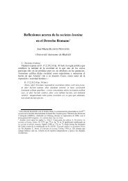
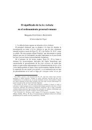
4.1. Uniform flow<br />
This first test case consists in a uniform flow<br />
(M ∞<br />
=0.2) through a rectangular duct. The goal is to<br />
check if the DGCL is satisfied and to measure the<br />
time evolution of the error for non-DGCL schemes.<br />
The grid is required to vibrate with a fixed pulsation<br />
ω=500π and several distorsion amplitudes. The<br />
numerical time step Δt is constant and is such that<br />
the mesh movement period is discretized on 16<br />
points.<br />
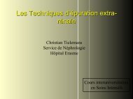
Realtive error<br />
2,51E-04<br />
2,01E-04<br />
1,51E-04<br />
1,01E-04<br />
5,10E-05<br />
dx0 = 0.05 h<br />
dx0 = 0.1 h<br />
dx0 = 0.15 h<br />
1,00E-06<br />
2,50E-04 2,00E-03 3,75E-03 5,50E-03 7,25E-03<br />
Time t (s)<br />
Figure 1. Time evolution of the relative error for<br />
the non respective DGCL Cranck-<strong>Nicolson</strong> scheme<br />
for different mesh distosion amplitudes.
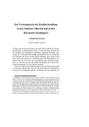
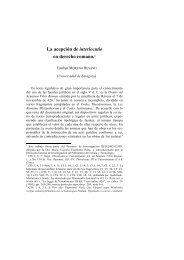
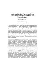
Relative error<br />
1,82E-12<br />
1,62E-12<br />
1,42E-12<br />
1,22E-12<br />
1,02E-12<br />
8,20E-13<br />
6,20E-13<br />
4,20E-13<br />
2,20E-13<br />
Distinct normals procedure<br />
Normal mean procedure<br />
2,00E-14<br />
2,50E-04 1,75E-03 3,25E-03 4,75E-03 6,25E-03<br />
Time t (s)<br />
Figure 2. Time evolution of the relative error for<br />
both the distinct normals and the normal mean<br />
approach for a mesh distorsion amplitude of dx0 =<br />
1.5 h.<br />
The relative error ε occurring at each time step<br />
is computed with the following formula<br />
ε =<br />
∑<br />
i<br />
( ui<br />
− u )<br />
∑ ( ui<br />
)<br />
i<br />
2<br />
i<br />
2<br />
(26)<br />
with u u<br />
i and<br />
i respectively denoting the numerical<br />
solution and the analytical solution.<br />
Figure 1 shows the evolution of error with time<br />
for the non modified Cranck-<strong>Nicolson</strong> scheme<br />
while Figure 2 shows it for both normal mean and<br />
distinct normals approaches.<br />
These examples clearly show that, as opposed<br />
to the non-DGCL Cranck-<strong>Nicolson</strong> scheme, either<br />
the normal mean and the distinct normals<br />
techniques lead to a DGCL scheme.<br />
4.2. Advection scalar test<br />
The accuracy analysis is here made by solving<br />
the following simple linear scalar hyperbolic<br />
conservation equation on a cubic domain.<br />
∂u<br />
∂u<br />
+ = 0<br />
∂t<br />
∂x<br />
(27)<br />
The initial condition consists in the continuous<br />
spherical field<br />
2⎛<br />
1 ⎞<br />
u = 1+<br />
cos ⎜ π r ⎟<br />
⎝ 2 ⎠ if r < 1<br />
(28)<br />
u = 1<br />
if r ≥ 1<br />
(29)<br />
with the radius r defined as<br />
r =<br />
2<br />
2<br />
( x − 0.3) + ( y − 0.5) + ( z − 0.5)<br />
with R=0.25.<br />
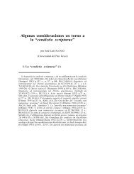
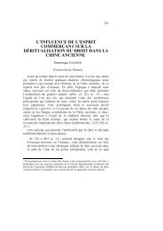
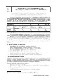
Error<br />
7.50E-03<br />
6.50E-03<br />
5.50E-03<br />
4.50E-03<br />
3.50E-03<br />
2.50E-03<br />
1.50E-03<br />
R<br />
Violating DGCL scheme<br />
Distinct normal scheme<br />
Normal mean scheme<br />
Fixed grid error limit<br />
2<br />
(30)<br />
5.00E-04<br />
2 4 8 16 32 64<br />
T/(2dt)<br />
Figure 3. Time integration error on a vibrating grid<br />
for the respecting DGCL schemes (distinct normal<br />
and normal mean procedures) and for the non<br />
modified Cranck-<strong>Nicolson</strong> scheme violating the<br />
DGCL.<br />
The analytical solution is simply a translation of<br />
that initial field in the x direction with a unitary<br />
speed. For accuracy analysis, the numerical solution<br />
u obtained at t=0.08 with a time step Δt=2.5 is<br />
compared with the analytical solution u on each<br />
node i for the different procedures. The relative<br />
error ε is computed by Eq. (26).<br />
Here, the distorsion amplitude Δx 0<br />
is maintained<br />
constant for each test while the vibration period T of<br />
the grid movement goes from small to large number<br />
of time steps. Figure 3 shows the different errors<br />
obtained for each procedure.<br />
This example highlights that the non modified<br />
Cranck-<strong>Nicolson</strong> scheme, which does not meet the<br />
DGCL, exhibits larger errors for the high frequency<br />
mesh movements and that its behaviour depends of<br />
how the mesh movement is time discretized. On the<br />
other hand the two DGCL schemes are less<br />
dependent of the grid velocity. Finally we can also<br />
observe that the obtained error for very slow mesh<br />
motions tends to be equal to the fixed grid error<br />
whether the scheme is DGCL or not. This remark<br />
means that satisfying the DGCL is really essential<br />
when the characteristic time of the grid movement<br />
becomes comparable or smaller that the numerical<br />
time step.
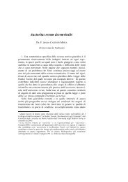
4.3. Steady plane flow in a channel with a<br />
bump using a 3D vibrating mesh<br />
A steady subsonic flow (M ∞<br />
=0.3) in a channel<br />
with a bump is computed on a tetrahedral mesh<br />
(19378 cells) and serves as initial field before the<br />
mesh starts to vibrate.<br />
Number of Krylov vectors<br />
35<br />
30<br />
25<br />
20<br />
15<br />
10<br />
5<br />
0<br />
NM-dx0=h<br />
DN-dx0=h<br />
NM-dx0=0.5 h<br />
DN-dx0=0.5 h<br />
NM-dx0=0.25 h<br />
DN-dx0=0.25 h<br />
1 2 3 4 5 6<br />
Nonlinear iterations<br />
Figure 4. Convergence curves : number of Krylov<br />
vectors per nonlinear <strong>New</strong>ton iterations for several<br />
mesh distorsion amplitudes (Δx 0<br />
= 0.25h, Δx 0<br />
= 0.5h<br />
and Δx 0<br />
= h) using the normal mean procedure (MN)<br />
and the distinct normals procedure (DN).<br />
The only unsteadyness is here brought by the<br />
mesh movement. Figure 4 shows the necessary<br />
number of Krylov vectors within each nonlinear<br />
<strong>New</strong>ton iteration until the convergence is obtained<br />
from the numerical solution at time t n to the new<br />
solution at time t n+1 .<br />
For a random Δx 0<br />
= 0.25h distorsion, both mean<br />
normal and distinct normals approaches exhibit the<br />
same behaviour. However, for a Δx 0<br />
=0.5h<br />
distorsion, the distinct normals approach shows an<br />
improved convergence rate. This becomes more<br />
critical for a Δx 0<br />
=h distortion. For the latter, it<br />
should be noted that even some mesh crossovers<br />
appear (about 4.8% of the volumes) ; this however<br />
doesn’t alter the conservativity of the finite volume<br />
discretization and solutions could be obtained by<br />
both methods on the cases presented here with such<br />
extreme conditions.<br />
showed an improved convergence rate with respect<br />
to a normal mean approach, with the same accuracy.<br />
This new technique could also be applied when the<br />
spatial coordinates explicitly appear in the fluxes<br />
expressions (e.g. Euler equations in cylindrical<br />
coordinates), which can’t be handled by mean<br />
normal procedure.<br />
Further investigations need of course to be<br />
carried out for unsteady flows with moving<br />
boundaries.<br />
REFERENCES<br />
[1] Thomas P.D., and Lombard C.K.,<br />
“Geometrical Conservation Law and its<br />
Applications to Flow Computations on Moving<br />
Grids”, AIAA Journal, 17:1030, 1979.<br />
[2] Guillard H., and Farhat C., “On the<br />
Significance of The Geometric Conservation Law<br />
for Flow Computations on Moving Meshes”,<br />
Comput. Meth. Appl. Mech. Eng., 190:1467, 2000.<br />
[3] Fromaggia L., and Nobile F., “A Stability<br />
Analysis for the Arbitrary Lagrangian Eulerian<br />
Formulation with <strong>Finite</strong> Elements”, East-West J.<br />
Numeric Math., 7:107, 1999.<br />
[4] Farhat C., Geuzaine P., and Grandmont C.,<br />
“The Discret Geometric Conservation Law and the<br />
Nonlinear Stability of <strong>ALE</strong> <strong>Scheme</strong>s for the<br />
Solution of Flow Problems on Moving Grids”,<br />
Journal of Computational Physics, 174:669, 2001.<br />
[5] Batina J.T., “Unsteady Euler Airfoil<br />
Solutions Using Unstructured Dynamic Meshes”,<br />
Jan 1989. AIAA Paper 89-0115.<br />
[6] Delanaye M., and YenLiu, “Quadratic<br />
Reconstruction <strong>Finite</strong> <strong>Volume</strong> <strong>Scheme</strong>s on 3D<br />
Arbitrary Unstructured Polyhedral Grids”, June<br />
1999. AIAA Paper 99-3259.<br />
[7] Lepot I., Meers F., and Essers J.-A.,<br />
“Multilevel Parallel High Order <strong>Scheme</strong>s for<br />
Inviscid Flow Computations on 3D Unstructured<br />
Meshes”, In Proceedings of the ECCOMAS<br />
Computational Fluid Dynamics Conference, Sep<br />
2001.<br />
5. CONCLUSION<br />
A geometrically conservative high order scheme<br />
has been presented. The importance of verifying the<br />
Discrete Geometric Conservation Law for<br />
computations on highly moving grids has been<br />
outlined on simple test cases.<br />
The new proposed DGCL enforcement has